A Stationary Planar Random Graph with
Singular Stationary Dual:
Dyadic Lattice Graphs
Abstract.
Dyadic lattice graphs and their duals are commonly used as discrete approximations to the hyperbolic plane. We use them to give examples of random rooted graphs that are stationary for simple random walk, but whose duals have only a singular stationary measure. This answers a question of Curien and shows behaviour different from the unimodular case. The consequence is that planar duality does not combine well with stationary random graphs. We also study harmonic measure on dyadic lattice graphs and show its singularity.
Key words and phrases:
Unimodular, random graphs, Whitney decomposition, hyperbolic model, Baumslag–Solitar, harmonic measure.2010 Mathematics Subject Classification:
Primary 05C81, 05C80, 60G50; Secondary 5C10, 60K37.1. Introduction
Since the study [4] of group-invariant percolation, the use of unimodularity via the mass-transport principle has been an important tool in analysing percolation and other random subgraphs of Cayley graphs and more general transitive graphs; see, e.g., [14, Chapters 8, 10, and 11]. These ideas were extended by [1] to random rooted graphs. For planar graphs, a crucial additional tool is, of course, planar duality. In the deterministic case, [14, Theorem 8.25] shows that every planar quasi-transitive graph with one end is unimodular and admits a plane embedding whose plane dual is also quasi-transitive (hence, unimodular). This was extended by [1, Example 9.6] to show that every unimodular random rooted plane graph satisfying a mild finiteness condition admits a natural unimodular probability measure on the plane duals; in fact, the root of the dual can be chosen to be a face incident to the root of the primal graph. The recent paper [2] makes a systematic study of unimodular random planar graphs, synthesizing known results and introducing new ones, showing a dichotomy involving 17 equivalent properties.
One significant implication of unimodularity is that when the measure is biased by the degree of the root, one obtains a stationary measure for simple random walk. This led Benjamini and Curien [5] to study the general context of probability measures on rooted graphs that are stationary for simple random walk. One aim has been to elucidate which properties hold without the assumption of unimodularity. In particular, Nicolas Curien has asked (unpublished) whether stationary random graphs have stationary duals; our interpretation of this is the following question:
Question 1.1.
Given a probability measure on rooted plane graphs (that are locally finite and whose duals are locally finite), let be the probability measure on rooted graphs obtained from choosing a neighbouring face of uniformly at random. If is stationary (for simple random walk), then is mutually absolutely continuous to a stationary measure?
In Question 1.1 and henceforth, we use ‘stationary’ to mean ‘stationary with respect to simple random walk’.
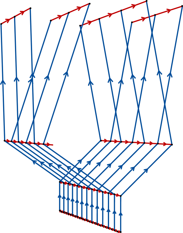
Here, we are actually interested in rooted plane graphs up to rooted isomorphisms induced by orientation-preserving homeomorphisms of the plane (though one could allow such a homeomorphism to change the orientation of the plane without affecting our results). In this paper, we give a negative answer in the general stationary case. This means that planar duality does not combine well with stationary random graphs. Our counterexample uses dyadic lattice graphs; the primal graphs have vertices of only two different degrees and the dual graphs are regular. See Figure 1.1 for a representation of a portion of the primal and dual graphs.
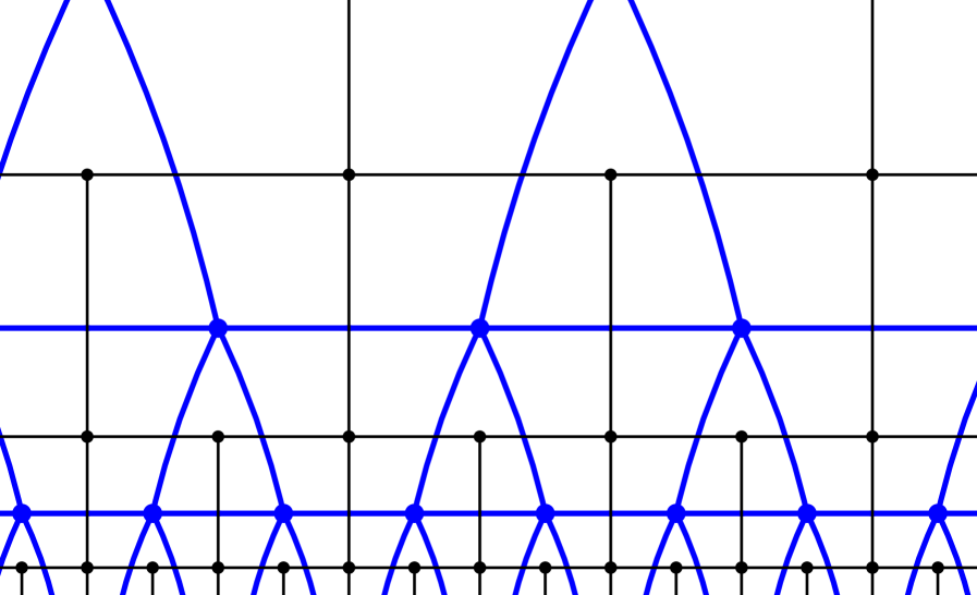
On the other hand, if the primal and dual graphs are both regular, then the resulting graphs are uniquely determined by their degrees and codegrees, are transitive, and are unimodular: see page 197 and Theorem 8.25 of [14]. In this sense, our counterexample is the best possible. See also the discussion of vertex and face degrees in Section 6. We do not have any examples, other than unimodular ones, of a stationary random plane graph with stationary dual; it seems possible there are none.
The dyadic lattice graphs we study are often used as a combinatorial approximation of the hyperbolic plane; see, e.g., the introductory work [8, Section 14]. Dyadic lattice graphs are also closely related to Whitney decompositions, which have been used in studying diffusions since the work of Bañuelos [3]. Finally, these graphs are subgraphs of the usual Cayley graph of the Baumslag–Solitar group —see Remark 2.11.
It might appear that there is only one dyadic lattice graph and only one dual. This is not true. While there is only one way to subdivide going downwards one level in the picture, there are two ways to agglomerate going upwards one level. Therefore, there are uncountably many such graphs. We will show, however, that there is a unique probability measure on rooted versions of such graphs that is stationary for simple random walk; the same holds for the duals. With appropriate notation, it is easy to put these measures on the same space; our main theorem is that these measures are mutually singular (Theorem 4.19). We also show that simple random walk tends downwards towards infinity and defines a harmonic measure. We will show that this measure is singular with respect to Lebesgue measure in a natural sense (Proposition 4.18).
We will not define ‘unimodular’ here because we will not use it again. In Section 2, we give crucial notation for the vertices in dyadic lattice graphs. This will also enable us to give useful notation to the entire rooted graph, which will identify a rooted dyadic lattice graph with a dyadic integer. That section also contains basic properties of dyadic lattice graphs that are invariant under automorphisms. In Section 3, we prove the fundamental existence and uniqueness properties of stationary and harmonic measures. In Section 4, we show how various symmetries of dyadic lattice graphs lead to (sometimes surprising) comparisons and identities for random-walk probabilities. We then use these to prove the singularity results mentioned above. We do not have explicit formulas for either the stationary measure on the primal graphs nor the harmonic measure for the primal graphs. Thus, in Section 5, we present some numerical approximations to these. Finally, Section 6 contains further discussion of the optimality of our example.
Sections 4 and 5 suggest several open questions. In particular, we do not know how to determine the stationary measure of even the simplest sets, or how to explain the patterns in the harmonic measure illustrated in Section 5.
Acknowledgements. We are grateful to the referees for their careful readings and questions, which led to improved clarity of our paper.
2. Notation and Automorphisms
We consider only planar embeddings of graphs that are proper, which means that every bounded set in the plane intersects only finitely many vertices and edges.
We will often work with left-infinite strings of binary digits. We will perform base-2 addition and subtraction with these strings, in which case the last (rightmost) digit is considered to be the units digit, and the place value of each other digit is twice as much as the digit to its right. For example,
We also have
We will use to denote appending digits to a left-infinite string, for instance,
Thus, we identify left-infinite strings of bits with the dyadic integers, . We may also write . Thus, for example, .
The symbol will indicate -fold repetition, so is the string .
We are interested in random walks on the following state space.
Definition 2.1.
Form a disconnected graph on the uncountable vertex set by adding an edge between the vertices and if either
-
•
and (such edges are called horizontal), or
-
•
and or and (such edges are called vertical).
The connected component of the vertex , with root , is denoted ; we endow with a planar embedding under which the sequence of edges , , has a positive orientation. While the set is uncountable, the connected component is countable, because each vertex has finite degree. Because every graph is -connected, every such planar embedding of is unique up to orientation-preserving homeomorphisms of the plane; see [10] or, for a simpler proof in our context, [14, Lemma 8.42 and Corollary 8.44]. The collection of such rooted embedded graphs is denoted ; they are in natural bijection with the dyadic integers, .
We say that the depth or level of the vertex is the integer .
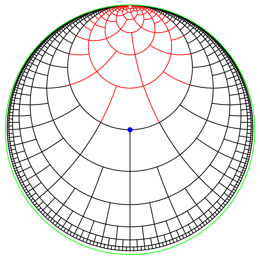
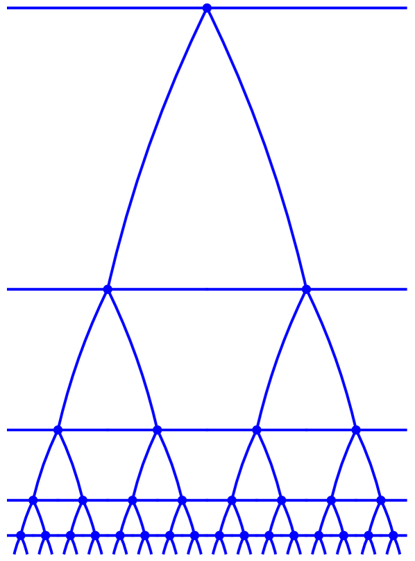
Figure 2.1 shows the local structure of the graph . The global structure of the graphs may be better seen in the Poincaré disc, rather than the upper halfplane, as in Figure 2.2.
For every , there is a rooted isomorphism from to given by . Here, negation is done in the additive group of dyadic integers, . This isomorphism clearly reverses the orientation specified by Definition 2.1.

Remark 2.2.
Two elements and of belong to the same connected component of iff there exists with or if both and are eventually 0 or 1, i.e., represent ordinary integers.
A simple random walk on is defined by simple random walk on the component of the starting vertex , that is, each vertex is a uniformly random neighbour of the preceding vertex, . This induces a walk on by projecting ; we regard this as a walk on rooted graphs, where we move the root from its present position to one of its neighbours, chosen uniformly at random. As we will see, there is an orientation-preserving rooted isomorphism between rooted graphs and iff .
Definition 2.3.
The simple random walk on the space of Definition 2.1 moves from the state to the state , where is obtained by choosing uniformly at random from either the following three or four options, depending on whether the last is valid.
-
•
Adding to (referred to as moving right).
-
•
Subtracting from (referred to as moving left).
-
•
Appending to (referred to as moving down).
-
•
Removing a terminal from (only possible if = 0) (referred to as moving up).
The behaviour of this random walk will be analysed by considering the following graph.
Definition 2.4.
Let be the graph whose vertex set consists of all finite strings of binary digits, including the empty string , with edges between vertices and if
-
•
(possible only if ), or
-
•
or .
Here, addition of to a string of length is reduced modulo , so that for instance
The depth or level of a vertex is the length of its string.
We will mostly be interested in what happens as the depth increases, because the depth of the simple random walk on has positive drift (Proposition 3.3). Again, -connectivity implies that there are at most two planar embeddings of up to planar homeomorphisms, but, in fact, there is only one, because reversing the orientation leads to an equivalent embedding: compare Proposition 2.6.
In comparing the definitions of and , observe that the depth of a vertex in is the length of the corresponding string, which in the finite setting can be read from the string and need not be given as an additional parameter as in the definition of .
The relation between the graphs and is that a portion of may be ‘wrapped’ to produce , as follows.
Remark 2.5.
The portion of induced by all vertices of nonnegative depth is denoted ; it does not depend on the choice of up to (orientation-preserving) rooted isomorphism. If we identify all pairs of vertices and of such that and for all , then the resulting graph is isomorphic to . We may also express the relationship between and as follows. For each , there is an automorphism of given by , where . The orbit of each vertex in corresponds to a single vertex of . We thus refer to as the quotient of by this action of .
This construction of does two things to —it removes the portion of the graph with negative depth, and then wraps the remaining graph around a cylinder, so that moving sufficiently far to the right or left results in returning to where one started.
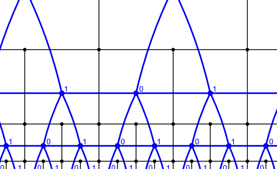
A portion of is shown in Figure 2.3 and also in Figure 2.4. Some key details are the following.
-
•
Each vertex has either degree or degree . (For the vertex , we consider each loop as contributing only to the degree.)
-
•
From any vertex, it is possible to move to the left or right. Moving in either direction alternates between vertices of degree and vertices of degree , except from .
-
•
From any vertex, it is possible to move down, to a vertex of degree .
-
•
From a vertex of degree only, it is possible to move up. This may result in a vertex of degree either or .

In the notation of Definition 2.4, vertices of degree are those whose strings end with a zero. Moving to the right or left corresponds to adding or subtracting from the string, moving downward corresponds to appending a zero, and moving upwards to removing a zero from the end of the string. This last operation is only possible when the string ends with a zero, which is why these strings correspond to vertices of degree . (From the empty string, , the only allowable moves are to stay at —in either of two ways—or to append a .)
While the graphs and are very structured, they usually do not have many automorphisms. Our experience is that this comes as a surprise to all who initially hear of it; probably this is because people are used to thinking about , which has automorphism group .
Proposition 2.6.
The graph has only one nontrivial automorphism.
Proof.
The graph has an automorphism that takes a binary string of length to the binary string of equal length. This may be seen as a reflection in Figure 2.3, where it fixes each string of the form and , and interchanges the two horizontal intervals between these fixed points. Equivalently, moves to the left and moves to the right are swapped. This is also a reflection in the real axis in Figure 2.4.
This notion of interchanging the notions of right and left is evident in the action of at any fixed depth. The depth portion of may be seen as the Cayley graph of the additive group of integers modulo with generators . There is a unique nontrivial automorphism of this graph that preserves the identity, defined by writing an arbitrary element as a sum of generators and reversing the sign of each of these generators, producing . This operation of reversing the sign exchanges the roles of the generators and , or equivalently of right and left.
Any automorphism of must fix , which is the sole vertex with a double loop, must fix , which is the only vertex connected to , and must fix , which is the only vertex connected to by two edges. Finally, it must fix the only other neighbours of and , which are and . There are only two vertices connected to both and , namely, and . Therefore any automorphism of either fixes these two vertices or interchanges them.
To see that has no nontrivial automorphisms other than , it suffices to show that an automorphism of that fixes the vertices and must fix the entire graph, as automorphisms that swap and may be composed with .
If an automorphism of fixes each -bit string for some , then it fixes each -bit string that ends with a zero, and then also fixes each -bit string that ends with a one, because each string ending with a one is adjacent to different pairs of strings ending with zeros, as long as . This completes the proof. ∎
Most graphs do not have nontrivial automorphisms, even considering automorphisms of graphs rather than rooted graphs, which need not fix the root vertex. We will show that edges of can be classified as either vertical or horizontal from the isomorphism class of , as well as whether traversing a vertical edge moves up or down; whether traversing a horizontal edge moves right or left can then be determined from the planar orientation of the embedding. This will result in the following:
Proposition 2.7.
The sequence may be read from the oriented graph via the following procedure.
Lemma 2.8.
In any graph , the classification of edges as horizontal or vertical may be read from the graph structure, in other words, is preserved by automorphisms.
Proof.
Any horizontal edge is between a vertex of degree and a vertex of degree , so an edge with two degree- endpoints must be vertical.
Consider an edge between a vertex of degree and a vertex of degree . If is adjacent to two vertices of degree , then is a horizontal edge. Otherwise, let be the unique vertex of degree adjacent to . If a shortest path between and that does not go through has length , then is horizontal. Otherwise such a path has length and is vertical. Examples of these paths are shown in red and green, respectively, in Figure 2.6. ∎
Lemma 2.9.
In any graph , the notions of ‘up’ and ‘down’ may be read from the graph structure.
Proof.
Let be a vertical edge between two vertices and . There are exactly two paths between these two vertices that take one horizontal step, then one vertical step, then two horizontal steps. The initial vertex of these paths is above the final vertex. ∎
Lemmas 2.8 and 2.9 imply Proposition 2.7, whence the string is determined from the isomorphism class of the (rooted, oriented) graph . More precisely, there is an orientation-preserving rooted isomorphism between and if and only if , as claimed earlier.
Proposition 2.10.
A graph has nontrivial automorphisms if and only if the sequence is eventually periodic. In particular, if is not eventually periodic, then the map from vertices of to is injective.
Proof.
If there is an automorphism that takes to with or , then by Proposition 2.7, either or (as dyadic integers). Since and belong to the same connected component of , it follows from Remark 2.2 that is eventually periodic, whence so is .
Conversely, if is eventually periodic, then has a vertex where is periodic. Thus, without loss of generality, assume that itself is periodic. Choose so that . Then there is an orientation-preserving automorphism that takes to , namely, . ∎
Note that any automorphism of acts on the depths of vertices by addition of a constant, so automorphisms that do not fix the depth of every vertex must have infinite order. Note also that only has a nontrivial depth-preserving automorphism when contains vertices labelled by strings of only zeros (the vertices on the axis of reflection), in which case there are also automorphisms that do not preserve depth. Therefore, the automorphism group of is only ever trivial or isomorphic to or , with the last case arising only when contains vertices labelled by strings of only zeros. In no case is even close to vertex-transitive.
Remark 2.11.
All our graphs () are subgraphs of the standard Cayley graph of the Baumslag–Solitar group . A portion of this Cayley graph is shown in Figure 2.7.
For comparison with our graphs, this Cayley graph is drawn with edges corresponding to the generator horizontal and edges corresponding to the generator vertical. The faces in our graphs have degree and correspond to the relation . This may be understood as saying that from any point, stepping up, right, down, left, and left again results in a cycle, returning to the starting vertex.
The primary difference is that in , one is permitted to step upwards only from every second vertex in a given level, whereas in the graph of , it is possible to step upwards from any vertex, but doing so from even or odd vertices result in different branches of the graph.
A choice of rooted graph , identifying the root of with the identity element of , amounts to choosing a ‘sheet’ in the Cayley graph of the group , where it is always possibly to move downward or sideways, but at each level only one of the two upward branches (even or odd) is chosen.
3. Stationary and Harmonic Measures: Basic Properties
We will consider simple random walks on and . Both of these random walks tend downward. The depth of the walk on tends to ; consequently, on , the strings that represent the location of the walk have length tending to .
Definition 3.1.
Consider a random walk on either or . For each integer , let the random variable be the last time for which the depth of the walk is at most . That is, at time , the depth is and at each time after , the depth is greater than . If there are arbitrarily large times for which the depth is at most , then . We call the leaving time for depth .
Proposition 3.2.
The simple random walks on or starting at depth have the property that are IID with distribution not depending on , and are independent of . Also, there exists such that for every , we have . The distribution of is the same for simple random walks on as on .
To prove this, we first obtain bounds on the drift. From a vertex of degree , it is equally likely that the walk moves up or down, while from a vertex of degree , only down is an option. Thus, the drift comes from moves downward from vertices of degree . Write for the depth of a vertex of or .
Proposition 3.3.
Let be simple random walk on or , with any choice of . Let be the depth of . Then
and for all ,
Proof.
By considering all possible sequences of two steps from the vertex , we calculate that
Thus, in all cases. Since the random variables are uncorrelated and take values in for , the strong law of large numbers yields that their average tends to 0 a.s.; see, e.g., [14, Theorem 13.1]. This gives the first result. Moreover, are martingale differences, whence the Hoeffding–Azuma inequality yields
Proof of Proposition 3.2.
Note that each level is reached for the first time at a vertex of degree 4, except possibly for the starting level. The portion of the graph at the levels equal to or greater than that of a given vertex and rooted at that vertex does not depend on that vertex or on which graph in the walk takes place, in the sense that it is the same up to rooted isomorphism, so are IID in and have distribution independent of . Likewise, for the random walk on , the random variables are IID in ; in addition, a walk on projects to a walk on in a way that preserves changes in levels, whence the distribution of is the same on as on . Finally, let be the first time the random walk is at level . For ,
and
whence exponential tail bounds are provided by Proposition 3.3. ∎
We are interested in the following features of the limiting behaviour of the simple random walks on and . As mentioned earlier, we sometimes identify with the set of dyadic integers.
Definition 3.4.
A stationary (probability) measure for simple random walk on is a probability measure on the dyadic integers that is stationary for the induced random walk. We will show that there is a unique such probability measure and denote it by .
We will show in Proposition 3.7 that simple random walk on , considered as a sequence of finite binary strings, converges coordinatewise a.s. to a right-infinite string. Any given infinite string will be such a limit with probability 0 by Lemma 3.9, so there is no loss of information if we identify a right-infinite string with the number in of which it is a binary representation. With this identification, the convergence of a path in to an element of may be seen as convergence of the horizontal position in Figure 2.3. It will be convenient to use this position to describe certain vertices—for example, the vertices are at for all . We may also identify with .
Definition 3.5.
The harmonic measure for simple random walk on starting at the vertex is the probability measure on the real interval that is the law of the limit of the horizontal positions of the walk. We use for this measure.
To interpret the horizontal position of the walk as a point in , refer to Figure 2.3. Horizontal steps at depth have size , and the graph is wrapped around a cylinder so that the left and right sides are identified—these are the horizontal positions and .
Because is the quotient of by , we may denote the vertices in by , where and is a vertex of . Here, the inverse image of under the quotient map is , which are assumed ordered from left to right. If has horizontal position , then we identify with . We will also refer to as the horizontal position of .
Definition 3.6.
The harmonic measure for simple random walk on starting at the vertex is the probability measure on that is the law of the limit of the horizontal positions of the walk.
The quotient map from to pushes forward the random walk on to the random walk on , whence it also pushes forward to . We sometimes regard as a measure on and correspondingly as a measure on .
Proposition 3.7.
The harmonic measures and are well defined, in the sense that random walks on and on can be considered to converge a.s. to elements of or , respectively. Furthermore, the support of is and for every path in and every , the probability is positive that the random walk on starting with has and has the property that for all , the horizontal position of differs from the horizontal position of by less than .
Proof.
Because is a quotient of , it suffices to prove that is well defined in order to prove that is well defined. For , let be the number of times that the random walk is at level and be the total (signed) change in horizontal position while at level . At most sideways steps are taken on level , and each of these changes the horizontal position by , so . By Proposition 3.2, , so . Because , it follows that . Therefore converges a.s., which is the result. Because the tails of are arbitrarily small, the rest of the proposition follows. ∎
An almost identical argument shows the following:
Lemma 3.8.
For every , there is an such that for every , the simple random walk on starting at has the property that with probability at least , we have for all that and the horizontal position of differs from the horizontal position of by less than . ∎
Lemma 3.9.
For every , and for every , .
Proof.
It suffices to prove the second statement. Fix . Define to be the first time after that the walk makes a horizontal step , and let be the level at which the walk makes that step. Because each is a.s. finite, we may choose an increasing sequence so that for each , we have . Let be the set of paths that tend to , so that . Let be the set of paths in for which , so that . Write for the sequences obtained from by changing the step to ; all sequences in still correspond to paths in , and . However, paths in tend to . Note that this limit depends on , which is not the same for all paths in . However, by the definition of the sequence , paths in and cannot have the same limit for . Therefore the sets () have disjoint sets of limits in , yet each of these sets has probability at least . Therefore, , as desired. ∎
Theorem 3.10.
There is a unique stationary measure on for simple random walk. Furthermore, is continuous, that is, every singleton has measure .
Proof.
The key idea is to consider a random walk on as developing a longer and longer past history, which converges to the stationary measure. Every time the random walk leaves a level for the last time, the future moves of the random walk are independent of the graph above that level, and therefore have the same distribution no matter what is. The existence of such regeneration times shows that there is at most one stationary measure. Furthermore, we can construct a stationary measure from them as follows. We break up the walk into segments between the last times it leaves successive levels. These segments are IID, and have finite expected length by Proposition 3.2. The usual length-biasing and uniform choice then yields a stationary process of random walk moves. These random walk moves must still be converted to dyadic integers. Whether the walk is presently at a vertex of degree or degree depends only on the most recent (partial) segment. If it is at a vertex of degree , then the degree of the vertex immediately above depends only on the most recent two segments, and so on. Considering increasing numbers of these segments will allow us to obtain the stationary measure as a limit. Lastly, the IID segments of random walk moves have distribution that is invariant under switching left and right moves; this leads to continuity of .
We now begin the proof. Consider simple random walk on starting at . Each transition is a move on that is either left, right, up, or down from the current position; code this as a symbol , where the walk moves from to via . The sequences are IID for . (Here, for all .) Let denote their common law. Because , we may define to be the distribution on defined by
and then to be the law of when is uniformly chosen from and has law . Let denote the law of , where is independent of the walk and has law . Consider now sequences of indexed by the nonpositive integers. Then renewal theory shows that the finite-dimensional distributions of tend as to those of the concatenation of (), where are independent for with law when and with law when . In particular, this is independent of . Indeed, the graph has cycles of length , whence the distribution of is nonlattice. Therefore, the discrete key renewal theorem shows that for the delayed renewal process with renewals at , the age distribution tends to . This gives convergence to the equilibrium renewal process; e.g., [13, Theorem 3.1]. Usually one looks into the future, but one can just as well look into the past, as we do here. Given this, the fact that the sequences are IID yields our claim.
We next convert these random walk moves to dyadic integers. Each finite sequence from corresponds to a function by composing the individual-symbol functions , , , , provided is applied only to even dyadic integers. Here, for a sequence , we compose in the order . Say that a finite sequence is ‘definable’ if satisfies that restriction when applied to every dyadic integer and is ‘permissible’ if for every nonempty initial segment of , the number of symbols is strictly larger than the number of symbols ; in particular, the first symbol of each permissible is . The sequences above are guaranteed to be both definable and permissible. Furthermore, the value of mod 2 does not depend on for definable and permissible . More generally, mod does not depend on for any definable and permissible sequences . Therefore, has a limit a.s. as and does not depend on ; its law is .
Finally, for , the moves in result in a net change to the depth of and in a net horizontal change compared to the location of . That is, we may write for some IID -valued random variables , where with the depth of . The law of is invariant under switching and , whence has the same law as . The law of the limit of is that of , a series that converges in the -adic metric by the estimates in the proof of Proposition 3.7. Now an argument very similar to that proving Lemma 3.9 shows that the law of is continuous, whence so is . ∎
Uniqueness of the stationary measure guarantees that is ergodic, i.e., every measurable set that is closed for the random walk has measure 0 or 1.
Corollary 3.11.
The set of eventually periodic has -measure 0.
Proof.
There are only countably many finite binary strings, whence there are only countably many eventually periodic strings. Thus, the result is immediate from Theorem 3.10. ∎
The following result shows that can be seen in the ‘tail’ of . It will be important for our proof of singularity (Theorem 4.19).
Proposition 3.12.
Let be a finite binary string of length . For -a.e. ,
Proof.
Corollary 3.11 says that almost no are eventually periodic, so for -a.e. , the map for vertices of is well defined in view of Proposition 2.10. Consider the stationary simple random walk on . If , then for each , there is some such that is a vertex of ; with the preceding notation, we may write . Given , we may (-a.s.) identify the walk with simple random walk on starting at its root, . Now consider the standard two-sided stationary extension of the stationary simple random walk on . Thus, has the same law as for every . Because the walk on drifts downward, this two-sided extension almost surely has the property that for every , the number of with is finite. Let be the list of times with , listed in increasing order. Thus, , with the leaving times of Definition 3.1.
Write . Lemmas 3.8 and 3.9, together with stationarity, imply that
Because one of the times is 0, we obtain
Let be the event that ; using the definition of and the fact given earlier that , the preceding equation can be written as
| (3.13) |
Let be the set of random walk trajectories where the level at time is never visited again. The law of is invariant and ergodic under the left shift because is invariant and ergodic, and the leaving times correspond to shifts that bring the trajectory to . Because the return map to is also measure-preserving and ergodic, it follows that the sequence is stationary and ergodic. Therefore, for each , the ergodic theorem yields
| (3.14) |
On the other hand, Proposition 3.7 shows that converges a.s. as with ; since by stationarity, is the same for all , we obtain
| (3.15) |
Since is a Cauchy sequence a.s., we have
By stationarity, does not depend on . Therefore,
Choosing , , and yields
| (3.16) |
Combining (3.14), (3.15), and (3.16), we obtain
which is the same as
In view of (3.13), we may write this as
This is the desired result. ∎
Unfortunately, we do not have an explicit description of . For instance, one may ask about the proportion of time a simple random walk spends on vertices of degree three.
Definition 3.17.
Given a random walk on or , denote by the limiting fraction of the time spent at vertices of degree .
The limit need not exist for general random walks on these graphs, but it will for the simple random walks we study.
Proposition 3.18.
For simple random walks on or , the limit exists a.s., is constant, and is the same for as for .
Proof.
Consider a simple random walk on or that starts at a vertex at depth . This random walk may be broken up into the segments between the leaving times and for , in addition to the initial segment up to time . By Proposition 3.2, the expected time in each such interval spent at vertices of degree is bounded, and the times spent at vertices of degree in each of these intervals are IID, except for the initial segment. Therefore the limit exists and is equal to the ratio of the average time spent at vertices at degree between times and to the average interval length . ∎
We may also write , which equals for every if is the random walk on when has law . This is a basic quantity in understanding the behaviour of simple random walk on . For example, the speed (drift downwards) of simple random walk on every graph in or on equals because the drift at each vertex of degree 3 is 1/3 while the drift at each vertex of degree 4 is 0. We can get some simple bounds on as follows.
Each vertex of either has degree or degree . If it has degree , then the vertex above it has either degree or . Let and be the proportions of time spent at vertices of degree whose upper neighbour has the appropriate degree. These quantities exist by similar arguments to Proposition 3.18. Note that
| (3.19) |
Consider a vertex chosen according to the stationary measure, and take a single step. The resulting measure is still the stationary measure, so considering the probability of being at a vertex of degree gives us that
| (3.20) | ||||
Therefore . It follows that the downward speed is at most 1/7:
Proposition 3.21.
The drift downwards of simple random walk on every graph in or on is at most . ∎
Remark 3.22.
Using the equations (3.19) and (3.20), we find that
Similarly, with being the probability of being at a degree vertex with a degree vertex above and a degree vertex above that, we have
Substituting the previous expression for gives that , which implies the slightly better bounds since . One might hope to perform increasingly more detailed versions of this calculation, obtaining better and better bounds. This does not seem feasible because when vertices are classified by their neighbourhoods of radius in this way, the number of different types of vertex grows exponentially in . For instance, our first calculation used the fact that taking a horizontal step from a vertex of degree results in a vertex of degree , and the next that taking a horizontal step from a vertex of degree is equally likely to contribute to or . However, at the next level of detail, we would need to consider two different types of vertices of degree —those where a sideways step contributes to , and those where it contributes to .
In Section 5, we will give much more precise numerical estimates by other methods.
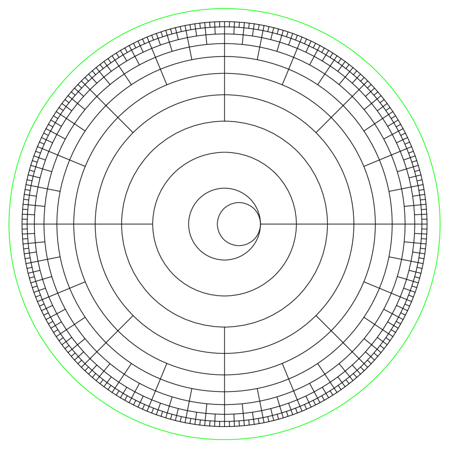
We now compare random walks on and to random walks on the dual graphs, where the ‘dual graph’ of is taken as the union of the dual graphs of the connected components of . The general shape of these dual graphs was shown in Figure 1.1. The appropriate analogue of in the dual setting is not the plane dual of , but rather is obtained from the dual of in the same way that was obtained from . Consider the dual of any graph , and define the graph to be the portion below any vertex, then ‘wrapped’ mod 1. This is shown in Figure 3.1. To avoid ambiguity, we will sometimes refer to , , and as the primal graphs, in contrast with their dual graphs.
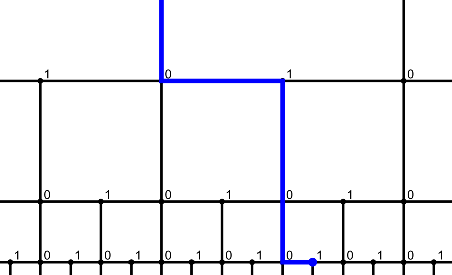
In , the faces are rectangular, each with five edges—one edge each on the top, left, and right sides, and two edges below. Therefore a step of the dual walk can go up, left, right, down-left or down-right. Denote by the collection of oriented, rooted, plane graphs dual to . It will be convenient to label the faces of (and hence the vertices of and of ) with binary strings (dyadic integers) in the same way as the vertices. We will label each face with the string labelling the vertex in its upper left corner, as shown in Figure 3.2.
With these labels, the dual walk on binary strings is defined as follows.
Definition 3.23.
To take a step of the dual walk, perform one of the following five operations, chosen uniformly at random.
-
•
Add or subtract .
-
•
Remove the final bit.
-
•
Append a or a .
Notice that the dual walk always allows a step upwards (removing the final bit), and has two different ways to step downward (appending either a or a )—compare to the primal walk of Definition 2.3. It is clear that the dual walk drifts downwards at speed 1/5.
We will also consider the stationary measure and the harmonic measure for the dual walk.
Definition 3.24.
A stationary (probability) measure for simple random walk on is a probability measure on the dyadic integers that is stationary for the induced random walk. Arguments similar to those used to prove Theorem 3.10 show that there is a unique stationary measure, .
In contrast to the primal case, we can easily identify . Namely, it is the symmetric Bernoulli process on , i.e., bits are independent fair coin flips.
Proposition 3.25.
The measure on is the product measure .
Proof.
This product measure is the same as Haar measure on the compact group, . Being Haar measure, it is invariant under both adding 1 and under subtracting 1, which correspond to the walk moving right or left. This measure is also clearly invariant under deleting the last bit, which happens when the walk moves up, and under concatenating a random fair bit, which is the fair mixture of moving down-left or down-right. Since this measure is invariant under each of these transformations, it is also invariant under the mixture of them given by a step of simple random walk. ∎
Definition 3.26.
The harmonic measure for simple random walk on starting at the top vertex is the probability measure on the real interval that is the law of the limit of the horizontal positions of the walk. Arguments similar to those used to prove Proposition 3.7 show that such a measure, , exists.
Again, we may identify explicitly as Haar (Lebesgue) measure on :
Proposition 3.27.
The harmonic measure for the dual walk is uniform on , equivalently, .
Proof.
It suffices to show that for each positive integer , this measure gives equal weight to the intervals for each between and .
To see this equality, for each path converging to a point in one of these intervals, we pair it with similar paths converging to points in each of the others. Define the dual leaving times as the last time the walk on is at depth . For each between and , at time the walk leaves depth for the last time. There are two equally likely ways this could be done, by appending or . Consider the family of paths obtained by making each combination of these independent choices, and otherwise moving as in . This grouping has the property that starting with any one of these paths produces the same set of paths.
At each time , these walks are at positions for some . If one of these walks converges to a point , then others converge to for each . This completes the proof. ∎
4. Graph Symmetries and Probabilities
The graph has only one nontrivial graph automorphism, described in Proposition 2.6. It interchanges the notions of ‘right’ and ‘left’ throughout the graph.
Proposition 4.1.
If is the reflection automorphism of Proposition 2.6, then the harmonic measure is -invariant.
Proof.
Automorphisms of any graph that fix the starting vertex leave the law of simple random walk invariant. ∎
Corollary 4.2.
If a number between and is chosen according to the harmonic measure , then for any positive integer , the probability that the th binary digit of is a is .
Proof.
Surprisingly, the generalisations of Corollary 4.2 to strings of more than one bit are false.
Proposition 4.3.
If a number between and is chosen according to the harmonic measure , then for any positive integer , the probabilities that the th and th binary digits of are or are equal, the probabilities of and are equal, and the former probabilities are strictly greater than the latter.
Intuitively, this is because if the random walk starts in the right half of Figure 2.4, then it is more likely to end up in the right half as well. Before we prove Proposition 4.3, we give some preliminary results. The proof appears after Proposition 4.14.
First, we define a reflection on random walk paths, as in Proposition 4.1. Unlike that reflection, this one will not be induced by an automorphism of the graph .
Definition 4.4.
Let be a path taken by the simple random walk on . Let be the first time greater than the leaving time at which is at a string of the form or (). It is possible that this never happens, in which case .
Define a modified path as follows.
-
•
If , then agrees with up until time , and then proceeds as except with left and right moves switched.
-
•
If , then .
We may regard as acting on the horizontal position by a reflection in either 1/4 or 3/4, whichever is visited first; in fact, these reflections are the same and implemented by the map . The map cannot be derived from an automorphism of , because it sometimes interchanges the vertices and , which have different degrees. However it only ever does this on a section of a path that never visits the vertex . Essentially, removing the vertex increases the available set of automorphisms. The reader may wish to review Figure 2.3.
Proposition 4.5.
Let be a path that is not fixed by and that converges to in the interval . Then converges to modulo .
Proof.
If a sequence of horizontal positions converges to , then the sequence converges to . ∎
Corollary 4.6.
If a path is not fixed by , then with probability exactly one of and converges to a binary string starting with or , while the other converges to a string starting with or .
Proof.
From Proposition 4.5, the map interchanges the open intervals and , in the sense that if converges to a point in and , then converges to a point in , and vice versa. Likewise, interchanges the intervals and .
The statement of the present corollary differs from this result only in that it refers to the half-open intervals , , , and , and requires only that the claim be true with probability . The probability that converges to any of the four points , or is zero by Lemma 3.9, which completes the proof. ∎
We will prove Proposition 4.3 by dividing paths into those fixed by , and others. Corollary 4.6 shows that paths not fixed by are as likely to converge to an element of the interval as to an element of the complement . It remains to consider paths that are fixed by .
Proposition 4.7.
If is a path that is fixed by and that does not converge to or , then there are two possibilities:
-
•
At time , is at . Then after time , only ever visits vertices beginning with or , and so converges to a string starting with or .
-
•
At time , is at . Then after time , only ever visits vertices beginning with or , and so converges to a string starting with or .
Proof.
In the first case, at time , the path is at . It never returns to depth , so the only way it could leave the set is via sideways moves. However, this would result in it passing through or . The path does not converge to or , so it contains a sideways move after this time, which contradicts .
The second case is the same but with the vertex and the set replaced by and . ∎
We will also need to show that the set of walks that are fixed by has positive probability.
Proposition 4.8.
Consider a simple random walk on that starts at . There is a positive probability that this walk eventually passes through the vertex , never returns to depth , and is fixed by .
Proof.
It suffices to show that the probability of a walk starting at never reaching a vertex of the form or is positive. This is immediate from Proposition 3.7. ∎
These probabilities of last leaving depth 1 at either vertex 0 or 1 are related to hitting probabilities in a surprising way—we will see that they are equal to the probabilities that a random walk started at or ever reaches the vertex . Because the random walk leaves depth from either or , these two probabilities sum to one. This will give the same relation for the hitting probabilities.
Definition 4.9.
Let be the set of paths from to . If , then this includes the path of length .
Definition 4.10.
If is a path, then is the probability of the path —that is, the product of the probabilities of each step, which is equal to the product of the reciprocals of the degrees of each vertex, except for the final vertex.
Definition 4.11.
The crest probability from a vertex of is the probability that the random walk, started from , ever reaches the vertex . Denote this probability by .
We now relate crest probabilities to the probabilities that a walk starting at leaves depth for the last time at or at , by reversing the paths in question.
Remark 4.12.
The probability (respectively, ) is equal to the probability that a walk starting at any vertex of degree (resp., ) ever reaches the level above its starting vertex.
Proof.
Consider random walks starting at (resp., ) and at any other starting vertex of degree (resp., ), and couple them so that they always move in the same direction—up, left, right, or down. Either both will eventually reach the level above their starting vertices, or neither will. ∎
Proposition 4.13.
The crest probabilities and are related by
In fact, for when .
Proof.
By the craps principle [15, p. 210], . By Remark 4.12, is the sum of over all paths that start at , end at , and do not visit again. Because , it follows that is the sum of over all paths that start at , end at , and do not visit again. This is the same as the sum of over all paths that start at , end at , and do not visit again, i.e., . ∎
These results generalise to the following.
Proposition 4.14.
For any depth , the sum of the crest probabilities from each of the vertices at depth is . For each vertex at depth , the crest probability satisfies when .
Proof.
The proof is the same as that of Proposition 4.13, with the vertex replaced by . ∎
Remark 4.15.
Using symmetry and the condition that equals the average of the values of at the neighbors of , one can show that , , and .
We have a similar extension to walks on :
Proposition 4.16.
Let be a vertex at depth of . The probability that simple random walk on started at and conditioned never to visit depth last leaves depth at equals the probability that simple random walk on started at visits before visiting any other vertex at depth (if any). ∎
While these techniques relating crest probabilities to the positions at which a random walk last leaves an appropriate set could be applied to other graphs, we note that Remark 4.12 requires that the graph in question be quite self-similar.
Proof of Proposition 4.3.
Note that the probabilities that the first two bits of are or are equal, as are the probabilities to be or , by the same argument as in Corollary 4.2. Thus it suffices to show that the probability of is greater than that of .
Combining Corollary 4.6 with Proposition 4.7, it suffices to show that the first case in Proposition 4.7 is strictly more likely than the second—that is, that among paths fixed by , more of them leave depth for the last time from the vertex than from the vertex . Now the probability of a path being fixed by is independent of its location at time . Therefore, the question reduces to showing that it is more likely to leave depth 1 from 0 than from 1. But these are the crest probabilities, for which this comparison is obvious because to return to from 1 it is necessary to pass through 0, so , and , where is the probability measure for the random walk starting at . ∎
Corollary 4.17.
The harmonic measure and the dual harmonic measure are not equal.
Proof.
Not only are these two measures not equal to one another, they are mutually singular.
Proposition 4.18.
The harmonic measure and dual harmonic measure are mutually singular.
Proof.
The harmonic measure is invariant under the left shift; in fact, we need a specific form of showing this invariance. Write for the limit of the random walk on . Write for the sequence of steps from taken by the random walk. Thus, is obtained from by applying the move . Then there is a measurable function such that . In fact, the same function gives all bits as . The sequences are IID for , as noted in the proof of Theorem 3.10. Therefore, is a factor of this IID sequence, so its law, , is ergodic, as is, obviously, . Two ergodic measures for the same transformation are either equal or mutually singular, whence the result. ∎
We remark that because is a factor of IID, it is isomorphic to what is called in ergodic theory a Bernoulli shift.
We may now answer Curien’s Question 1.1. Recall that and have a common coding by .
Theorem 4.19.
There is no stationary measure on that induces a measure on that is absolutely continuous with respect to some stationary measure.
Proof.
Both stationary measures are unique, so it suffices to show that the stationary measure on and the stationary measure on are mutually singular. Proposition 3.12 shows that -almost all binary strings have substring densities given by ; the same is evident for and by Propositions 3.25 and 3.27. Corollary 4.17 says that and are not equal, so and are mutually singular. ∎
5. Numerical Results
Because we do not have exact expressions for either or , we devote this section to numerical approximations. Some interesting patterns will emerge, leading to some open questions.
5.1. Numerical bounds on
One of the most interesting quantities is , the proportion of time spent at vertices of degree , well defined by Proposition 3.18. We do not know the exact value of , but the following sections give bounds on this quantity. Rough analytic bounds were obtained in Remark 3.22.
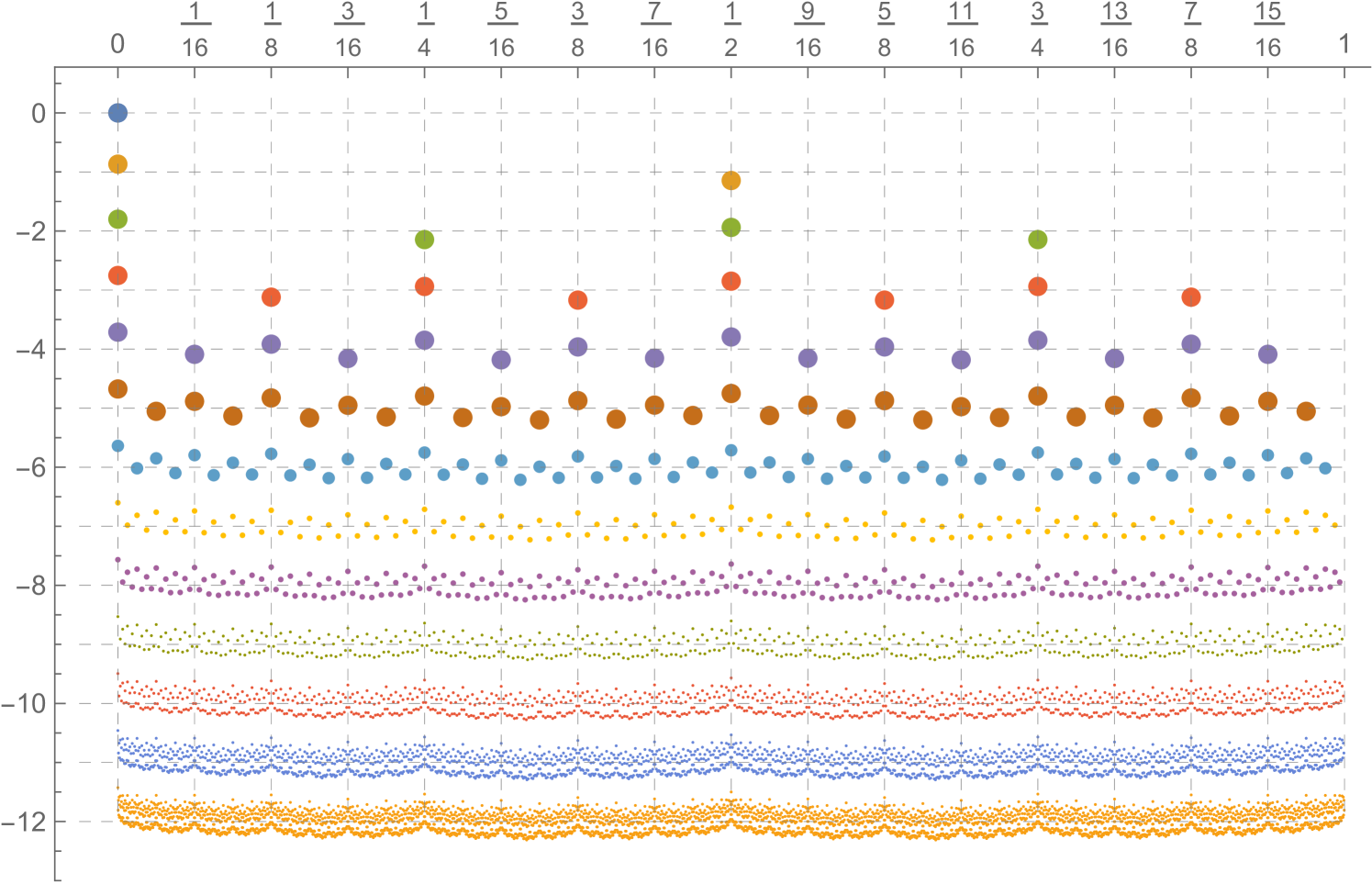
We begin with a discussion of the entire stationary measure, . An approximation of is shown in Figure 5.1. In order to show , we map by for . We then push forward via this map. We approximated by using the corresponding Markov chain on binary strings of length 12; removing the first bit corresponding to a move upwards entailed adding a last bit, which we fixed to be 0. We aggregated the stationary measure for this finite system into blocks of the first 6 most significant bits. Multiplying each of those numbers by shows it as a density in Figure 5.1. While we do not know how accurate these probabilities are, they appear surprisingly accurate if we can judge by the implied aggregate estimate of , which would be about ; this differs by only from our best estimate of using another method explained in the next two paragraphs. In any case, one can show that as the length used for the binary strings in this finite system grows, the error decays exponentially in that length. Also, because we used always 0 when a new last bit was needed, one might expect that the resulting estimate of would be a lower bound; however, we do not know a proof of this.
Notice that the speed is the probability of never returning to the current level, because each level is left for the last time just once. On the other hand, this nonreturn probability is equal to . Equating these two expressions for the speed, we obtain
Using this and an estimate , our estimate for is .
Our estimate for was obtained by the following method. The function , defined on the set of vertices of , is the solution to the Dirichlet problem with and . In other words, if is the graph induced by vertices in whose depth is between 0 and and is the harmonic function on with and for all of depth , then pointwise. Here, ‘harmonic’ means that is the average value of at the neighbours of for every whose depth is between 1 and . In addition, increases in . The function solves a sparse linear system of equations, which we solved for . We show for of depth at most 12 in Figure 5.2. There is a clear pattern based on the least significant bits; this is explained by Remark 4.12. Despite Proposition 4.14, the sum is not 1, but only tends to 1 as . Thus, we normalised to sum to 1 on each level. The last 14 of the resulting numbers seemed to be approaching a limit exponentially fast with ratio 2, so we fit such a curve to them, leading to our estimate of the preceding paragraph. One can show that does approach exponentially fast; one can also get an upper bound on by solving the Dirichlet problem where the values for of depth are set to an upper bound on for such .
5.2. Exploration of the harmonic measure
In this section, we investigate further the harmonic measure, , for simple random walk on . We know from Proposition 4.18 that is singular with respect to Lebesgue measure. Because is the quotient of by , it follows that is also singular with respect to Lebesgue measure on .
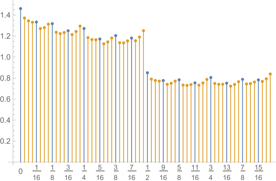
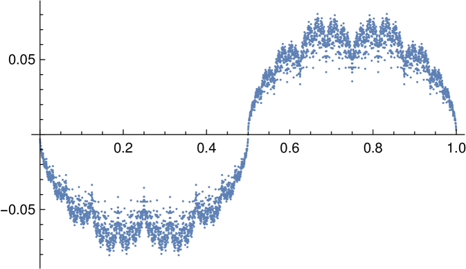
Figure 5.3 shows an approximation to . The figure has one dot for each interval of length , whose ordinate denotes the measure of that interval times , as if it were a density. Note that because is singular, finer approximations would tend to 0 and a.e. with respect to Lebesgue measure. We calculated this approximation as follows. Consider simple random walk on starting at depth 0. Let be the change in horizontal position between times and for . The reasoning behind Proposition 3.2 shows that are IID. Note that . The distribution of is ; taking this modulo 1 yields . Thus, it suffices to know the law of . By Proposition 4.16, equals the probability that simple random walk starting at at depth visits before visiting any other vertex at depth , where and . This is a solution to a Dirichlet problem again; we approximated it by the corresponding Dirichlet problem on between depths and , finding the probability for each of depth that random walk from visits before visiting any other vertex at depth or any vertex at depth . We normalised these probabilities to add to 1. Having this approximation to the law of at hand, we approximated the law of and then aggregated to intervals of length .
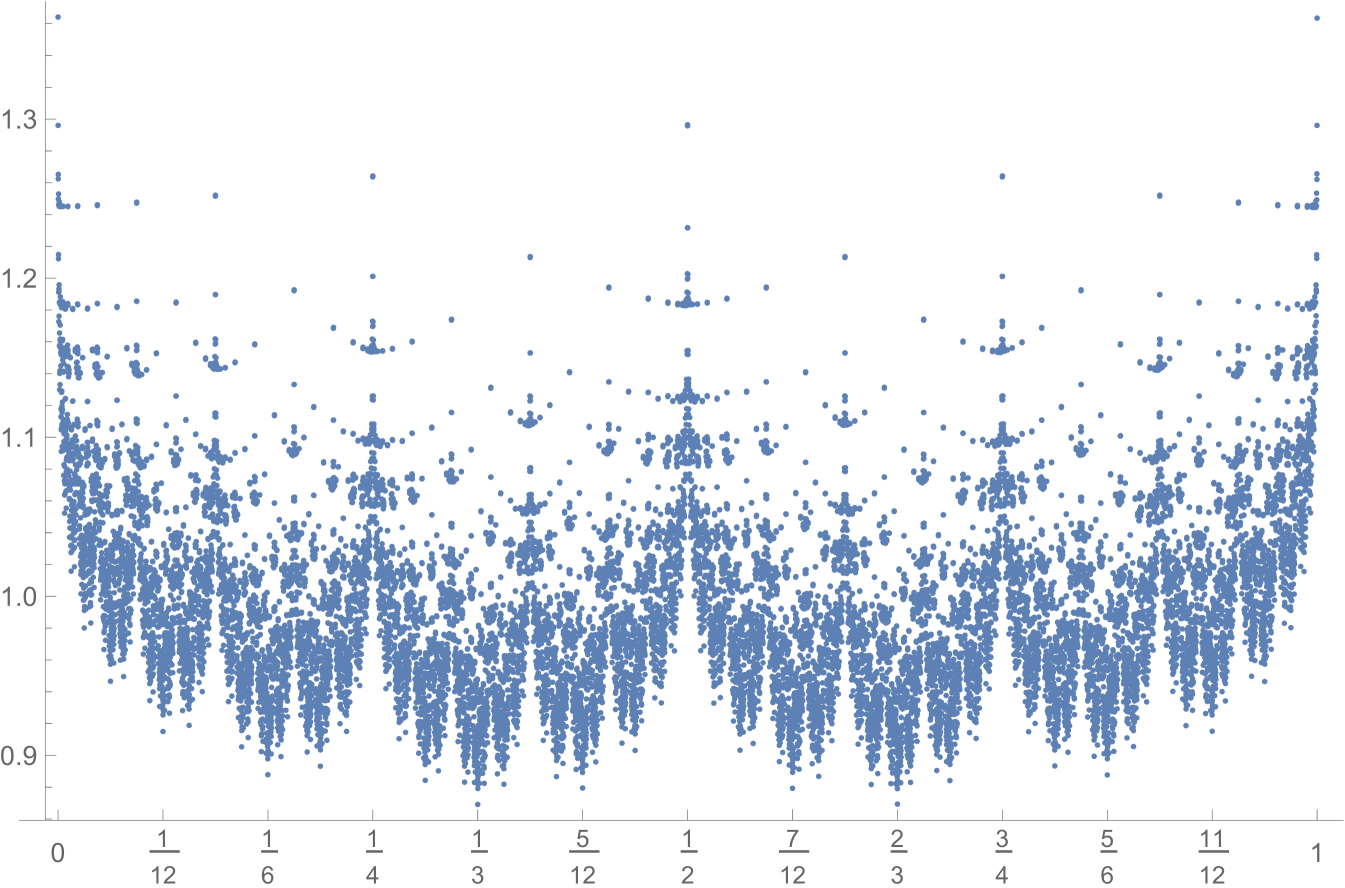
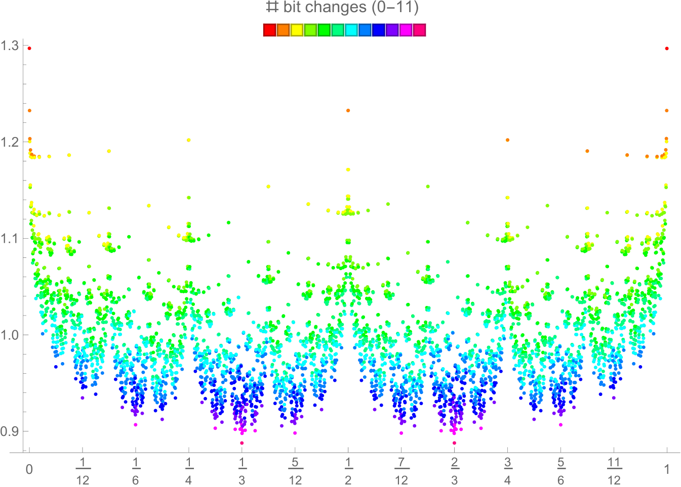
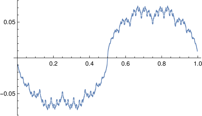
The locations of the most extreme maxima and minima in Figure 5.3 appear to be controlled by binary representations. Maxima occur at positions whose binary expressions are short and terminate, like and . Minima occur at positions whose binary expressions end in alternating sequences of ’s and ’s, like , , and . Figure 5.4 shows the same plot as Figure 5.3, but with intervals of length instead of and with colours corresponding to the number of differences in successive bits in the string of length 12. One can explain such a relationship by the use of -measures; see below.
While is self-similar in that it is invariant under the map , Figure 5.3 appears to show a different kind of self-similarity—the portion of the graph between and exhibits a similar pattern of oscillations to the whole graph. This indicates a weak influence of the first bit on the distribution of the remaining bits. We look at this quantitatively next.
For and , consider the conditional probability . This is defined for -a.e. . If we write as a binary string , then is the -probability that given . The base-2 entropy of equals
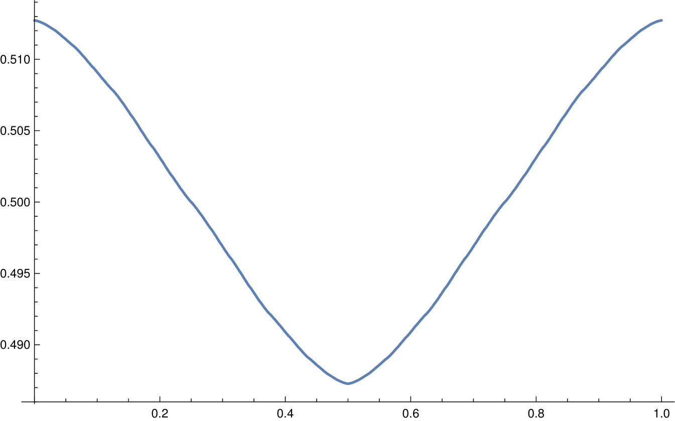
where is defined -a.e. The entropy is also the Hausdorff dimension of : there is a set of dimension that carries , but no set of dimension smaller than carries [6]. Because is invariant under the map , yet is not equal to Lebesgue measure, it follows that . Figure 5.5 shows an approximation to the function using points. This calculation used the approximation to mentioned above. Using our approximations of and , this gives . However, entropy is notoriously difficult to estimate, so although we have other methods that support this estimate of , we cannot claim great confidence in it. Interestingly, Figure 5.5 appears to show a continuous curve, monotone on each half of the interval. If such a curve really does exist, then harmonic measure is called a -measure [11]. This curve appears to have bounded variation with its derivative being a singular measure: see Figure 5.6. Proposition 4.1 shows that . Also, by definition. We believe that not only is continuous and monotone decreasing on , but that it determines uniquely as a -measure; see [12, 16, 7] for discussions of uniqueness.
Assuming that is continuous and appears as in Figure 5.5, we have that for and for . Therefore, will tend to be large at with for most (the same as the first two bits of being the same), i.e., for with few changes in successive bits, and will tend to be small at with for most (the same as the first two bits of being different), i.e., for with many changes in successive bits. This would explain Figure 5.4.
6. Optimality of the Construction
In this section, we show that any graph which is a counterexample to our main question must have either some vertices of degree at least or some faces of degree at least . Our graphs have vertices of degrees and and faces of degree .
Proposition 6.1.
If an infinite plane graph has vertices only of degree at most and faces only of degree at most , then the number of vertices of degree is at most .
Proof.
We use the combinatorial curvature of a vertex, defined to be minus half of the degree plus the sum of the reciprocals of the degrees of the incident faces. By Corollary 1.4 of [9], the sum of the combinatorial curvatures over all vertices is at most , and at most if the graph is infinite.
Write the combinatorial curvature at a vertex as plus the sum over all faces incident to of . The assumptions that vertex and face degrees are at most imply that the curvature at each vertex is at least , with equality if and only if the vertex has degree and all its incident faces are squares. The curvature is at least for a vertex of degree . This shows that there are at most vertices of degree . ∎
Corollary 6.2.
If an infinite plane graph has vertices only of degree at most and faces only of degree at most , then the number of vertices of degree plus the number of triangular faces is at most .
Proof.
Apply Proposition 6.1 to the graph formed from the primal and dual together, with new vertices of degree where the primal and dual edges cross. This new graph has one vertex of degree for each primal vertex of degree and one vertex of degree for each triangular face. ∎
The upper bound of is sharp, as can be seen by taking a triangular cylinder formed of squares that is infinite in one direction and capped by a triangle at the other.
Corollary 6.3.
The only stationary infinite plane graph whose vertices and faces have degree at most is the square lattice.
Proof.
Corollary 6.2 shows that such a graph can have only finitely many vertices and faces whose degree is not . If it is to be stationary, then it must have either zero or infinitely many such vertices and faces, so all vertices and faces have degree . In this case, the graph is the square lattice. ∎
References
- [1] David Aldous and Russell Lyons. Processes on unimodular random networks. Electron. J. Probab., 12:no. 54, 1454–1508, 2007. Errata, Electron. J. Probab., 22:no. 51, 4pp., 2017 and Electron. J. Probab., 24:no. 25, 1–2, 2019.
- [2] Omer Angel, Tom Hutchcroft, Asaf Nachmias, and Gourab Ray. Hyperbolic and parabolic unimodular random maps. Geom. Funct. Anal., 28(4):879–942, 2018.
- [3] Rodrigo Bañuelos. On an estimate of Cranston and McConnell for elliptic diffusions in uniform domains. Probab. Theory Related Fields, 76(3):311–323, 1987.
- [4] I. Benjamini, R. Lyons, Y. Peres, and O. Schramm. Group-invariant percolation on graphs. Geom. Funct. Anal., 9(1):29–66, 1999.
- [5] Itai Benjamini and Nicolas Curien. Ergodic theory on stationary random graphs. Electron. J. Probab., 17:paper no. 93, 20, 2012.
- [6] Patrick Billingsley. Ergodic Theory and Information. John Wiley, New York, 1965.
- [7] Maury Bramson and Steven Kalikow. Nonuniqueness in -functions. Israel J. Math., 84(1-2):153–160, 1993.
- [8] James W. Cannon, William J. Floyd, Richard W. Kenyon, and Walter R. Parry. Hyperbolic geometry. In Silvio Levy, editor, Flavors of Geometry, volume 31 of Mathematical Sciences Research Institute Publications, pages 59–115. Cambridge University Press, Cambridge, 1997.
- [9] Matt DeVos and Bojan Mohar. An analogue of the Descartes-Euler formula for infinite graphs and Higuchi’s conjecture. Trans. Amer. Math. Soc., 359(7):3287–3300, 2007.
- [10] Wilfried Imrich. On Whitney’s theorem on the unique embeddability of -connected planar graphs. In Miroslav Fiedler, editor, Recent Advances in Graph Theory (Proc. Second Czechoslovak Sympos., Prague, 1974), pages 303–306. (Loose errata). Academia, Prague, 1975.
- [11] Michael Keane. Strongly mixing -measures. Invent. Math., 16:309–324, 1972.
- [12] François Ledrappier. Principe variationnel et systèmes dynamiques symboliques. Z. Wahrscheinlichkeitstheorie und Verw. Gebiete, 30:185–202, 1974.
- [13] Torgny Lindvall. Lectures on the coupling method. Dover Publications, Inc., Mineola, NY, 2002. Corrected reprint of the 1992 original.
- [14] Russell Lyons and Yuval Peres. Probability on Trees and Networks, volume 42 of Cambridge Series in Statistical and Probabilistic Mathematics. Cambridge University Press, New York, 2016.
- [15] Jim Pitman. Probability. Springer, New York, 1993.
- [16] Örjan Stenflo. Uniqueness in -measures. Nonlinearity, 16(2):403–410, 2003.