A statistical framework for analyzing activity pattern from GPS data

Haoyang Wu, Yen-Chi Chen, Adrian Dobra
Contact: yenchic@uw.edu The authors gratefully acknowledge the support of NSF DMS-2310578, DMS-2141808 and NIH U24-AG072122.

Abstract

We introduce a novel statistical framework for analyzing the GPS data of a single individual. Our approach models daily GPS observations as noisy measurements of an underlying random trajectory, enabling the definition of meaningful concepts such as the average GPS density function. We propose estimators for this density function and establish their asymptotic properties. To study human activity patterns using GPS data, we develop a simple movement model based on mixture models for generating random trajectories. Building on this framework, we introduce several analytical tools to explore activity spaces and mobility patterns. We demonstrate the effectiveness of our approach through applications to both simulated and real-world GPS data, uncovering insightful mobility trends.

Keywords: GPS, nonparametric statistics, kernel density estimation, random trajectory, activity space, mobility pattern

1 Introduction

The rapid advancement of Global Positioning System (GPS) technology has revolutionized various domains, ranging from transportation and urban planning to environmental studies and public health (Papoutsis et al., , 2021; Yang et al., , 2022; Mao et al., , 2023). GPS data provides high-resolution spatial and temporal information, enabling precise tracking of movement and location patterns. With the increasing availability of GPS-equipped devices, such as smartphones, vehicles, and wearable deices, vast amounts of trajectory data are generated every day.

In scientific research, GPS data play a crucial role in understanding human mobility, tracing activity spaces, and analyzing travel behaviors (Barnett and Onnela, , 2020; Andrade and Gama, , 2020; Elmasri et al., , 2023). Researchers leverage GPS data to study commuting patterns, urban dynamics, wildlife tracking, and disaster response. By examining spatial-temporal GPS records, scientists gain insights into mobility patterns of individuals and the dynamics of population movements. Despite the rich information embedded in the GPS data, little is known about how to properly analyze the data from a statistical perspective.

While various methods exist for processing GPS data, a comprehensive statistical framework for analysis is still lacking. Traditional approaches often rely on heuristic methods or machine learning techniques (Newson and Krumm, , 2009; Early and Sykulski, , 2020; Chabert-Liddell et al., , 2023; Burzacchi et al., , 2024) that may lack rigorous statistical foundations. A major challenge in modeling GPS data is that records cannot be viewed as independently and identically distributed (IID) random variables. Thus, a conventional statistical model does not work for GPS records. The absence of a reliable statistical framework hinders cross-disciplinary applications and reduces the potential for scientific applications.

The objective of this paper is to introduce a general statistical framework for analyzing GPS data. We introduce the concept of random trajectories and model GPS records as a noisy measurement of points on a trajectory. Specifically, we assume that on each day, the individual has a true trajectory that is generated from an IID process. Within each day, the GPS data are locations on the trajectory with additive measurement noises recorded at particular timestamps. The independence across different days allow us to use daily-average information to infer the overall patterns of the individual.

1.1 Related work

Our procedure for estimating activity utilizes a weighted kernel density estimator (KDE; Chacón and Duong, 2018; Wasserman, 2006; Silverman, 2018; Scott, 2015). The weights assigned to each observation account for the timestamp distribution while adjusting for the cyclic nature of time, establishing connections to directional statistics (Mardia and Jupp, , 2009; Meilán-Vila et al., , 2021; Pewsey and García-Portugués, , 2021; Ley and Verdebout, , 2017).

Our analysis of activity space builds on the concept of density level sets (Chacón, , 2015; Tsybakov, , 1997; Cadre, , 2006; Chen et al., , 2017) and level sets indexed by probability (Polonik, , 1997; Chen and Dobra, , 2020; Chen, , 2019). Additionally, the random trajectory model introduced in this paper is related to topological and functional data analysis (Chazal and Michel, , 2021; Wang et al., , 2016; Wasserman, , 2018).

Recent statistical research on GPS data primarily focuses on recovering latent trajectories (Early and Sykulski, , 2020; Duong, , 2024; Huang et al., , 2023; Burzacchi et al., , 2024) or analyzing transportation patterns (Mao et al., , 2023; Elmasri et al., , 2023). In contrast, our work aims to develop a statistical framework for identifying an individual’s activity space and anchor locations (Chen and Dobra, , 2020). Activity spaces are the spatial areas an individual visits during their activities of daily living. Anchor locations represent mobility hubs for an individual: they are locations the individual spends a significant amount of their time that serve as origin and destination for many of the routes they follow (Schönfelder and Axhausen, , 2004).

1.2 Outline

This paper is organized as follows. In Section 2, we formally introduce our statistical framework for modeling GPS data. This framework describes the underlying statistical model on how GPS data are generated. Section 3 describes estimators of the key parameters of interest introduced in Section 2. Section 4 presents the associated asymptotic theory. To study human activity patterns, we introduce a simple movement model in Section 5 and present some statistical analysis based on this model. We apply our methodology to a real GPS data in Section 6 and explain the key insights about human mobility gained from our analysis. All codes and data are available on https://github.com/wuhy0902/Mobility_analysis.

2 Statistical framework of GPS data

Refer to caption — Figure 1: An example of real GPS data from an example individual (without timestamps). The four panels show the GPS records of this individual in four different days. The first three panels show weekdays whereas the last panel shows a weekend day. This is part of the GPS data that we analyze in Section 6.

We consider GPS data recorded from a single individual over several non-overlapping time periods of the same length. In what follows we will consider a time period to be one day, but our results extend to any other similar time periods that can be longer (e.g., weeks, months, weekdays, weekends) or shorter (e.g., daytime hours between 7:00am and 5:00pm).

The GPS data can be represented as random variables

(X_{i,j},t_{i,j})\in\mathbb{R}^{2}\times[0,1],

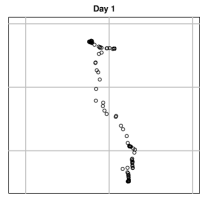
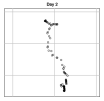
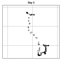
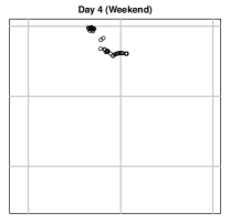
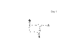
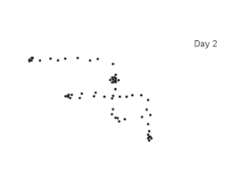
where $i=1,\ldots,n$ denotes the day in which the observation was recorded and $j=1,\ldots,m_{i}$ denotes the sequence of observations for $i$ -th day. Here $X_{i,j}$ stands for the spatial location of this GPS observation (latitude and longitude), and $t_{ij}$ represents the time when the observation was recorded. Note that for each day $i$ , $t_{i,1}<t_{i,2}<\ldots<t_{i,m_{i}}.$ Here $m_{i}$ is the total number of observations in day $i$ . We assume that the timestamps $t_{i,j}$ are non-random (similar to a fixed design). Figure 1 provides an example of real GPS data recorded from an individual in four different days (ignoring timestamps).

A challenge in modeling GPS data is that observations within the same day are dependent since each observation can be viewed as a realization of the individual’s trajectory on discrete time point (with some measurement errors). Thus, it is a non-trivial task to formulate an adequate statistical model that accurately captures the nature of GPS data.

2.1 Latent trajectory model for GPS records

To construct a statistical framework for GPS records, we consider a random trajectory model as follows. For $i$ -th day, there exists a continuous mapping $S_{i}:[0,1]\rightarrow\mathbb{R}^{2}$ such that $S_{i}(t)$ is the actual location of the individual on day $i$ and time $t$ . We call $S_{i}$ the (latent) trajectory of $i$ -th day.

The observed data is $X_{i,j}=S_{i}(t_{i,j})+\epsilon_{i,j},$ where $\epsilon_{i,j}$ is independent noises (independent across both $i$ and $j$ ) with a bounded PDF that are often assumed to be Gaussian. We also write $X_{R,i,j}=S_{i}(t_{i,j})$ to denote the actual location of the individual at time $t_{i,j}$ .

We assume that the latent trajectories $S_{1},\ldots,S_{n}\sim P_{S},$ where $P_{S}$ is a distribution of random trajectory. Namely, on each day, the individual follows a random trajectory independent of all other trajectories from $P_{S}$ . In Section 5, we provide a realistic example on how to generate a random trajectory.

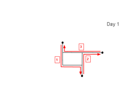
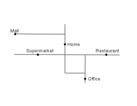
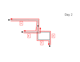
Figure 2 presents an example of the latent trajectory model. The first column presents a map of important locations such as home and office, and the corresponding road networks inside this region. The second column shows random trajectories of two days. The actual trajectory is shown in black lines. The red arrows indicate the direction of the trajectory. Note that the individual might remain at the same location for an extended period of time as indicated as the solid black dots in the second column. The third column presents the observed locations of the GPS records. We note that GPS records mostly follow the individual’s trajectory but may occasionally deviate from it due to measurement errors.

2.2 Activity patterns

The individual’s activity pattern is characterized by the distribution of the random trajectory $S(t)$ . Let $A\subset\mbox{$\mathbb{R}$}^{2}$ be a spatial region. The probability $P(S(t)\in A)$ is the probability that the individual is in the region $A$ at time $T=t$ . The manner in which distribution of $S(t)$ changes over time provides us with information about the dynamics of the most likely locations visited by this individual. Let $U\sim{\sf Uniform}[0,1]$ be a random variable independent of $S(t)$ . The probability

P(S(U)\in A)=\int_{0}^{1}P(S(t)\in A)dt.

can be interpreted the proportion of time that the individual spends in the region $A$ . Thus, the distribution of $S(U)$ tells us the overall activity patterns of the individual.

2.3 GPS densities

The distributions of $S(t)$ or $S(U)$ are difficult to estimate from the GPS data because of the measurement error $\epsilon$ . This is known as the deconvolution problem and is a notoriously difficult task. Thus, our idea is to use the distribution of $X_{t}=S(t)+\epsilon$ and $X^{*}=S(U)+\epsilon$ as surrogates.

Naively, one may consider the the marginal PDF of $X_{i,j}$

f_{X}(x)=\lim_{r\rightarrow 0}\frac{P(X_{i,j}\in B(x,r))}{\pi r^{2}}

(1)

as an estimate of the distribution of $X^{*}$ . This geometric approach (Simon, , 2014) is a convenient way to define density in this case. However, this PDF is NOT the PDF of $X^{*}$ because it depends on the distribution of the timestamps $T_{i,j}$ . Even if the individual’s latent trajectory remains the same, changing the distribution of timestamps $\{T_{i,j}:j=1,\ldots,m_{i}\}$ will change the distribution of $f_{X}$ .

Average GPS density. To solve this problem, we consider a time-uniform density of the observation. Let $U\sim[0,1]$ be a uniform random variable for the time interval $[0,1]$ . Recall that

X^{*}=S(U)+\epsilon,

where $S\sim P_{S}$ and $\epsilon\sim P_{\epsilon}$ are independent random quantities. $X^{*}$ can be viewed as the random latent position $S(U)$ corrupted by the measurement error $\epsilon$ . The average behavior of $X^{*}$ describes the expectation of a random trajectory (with measurement error) that is invariant to the timestamps distribution. With this, we define the average GPS density is the PDF of $X^{*}$ :

f_{GPS}(x)=\lim_{r\rightarrow 0}\frac{P(X^{*}\in B(x,r))}{\pi r^{2}}.

(2)

The quantity $f_{GPS}$ describes the expectation of a random trajectory with consideration to the measurement error and is invariant to the distribution of timestamps. What influences $f_{GPS}$ is the distribution of the latent trajectory $P_{S}$ and the measurement errors (which are generally small). Thus, $f_{GPS}(x)$ is a good quantity to characterize the activity pattern based on GPS records.

Interval-specific GPS density. Sometimes we may be interested in the activity pattern that takes place within a specific time-interval, e.g., the morning or evening rush hours. Let $A\subset[0,1]$ be an interval of interest. The activity patterns within $A$ can be described by the following interval-specific GPS density

$\displaystyle f_{GPS,A}(x)$	$\displaystyle=\lim_{r\rightarrow 0}\frac{P(X^{*}_{A}\in B(x,r))}{\pi r^{2}},$	(3)
$\displaystyle X^{*}_{A}$	$\displaystyle=S(U_{A})+\epsilon,$
$\displaystyle U_{A}$	$\displaystyle\sim{\sf Uniform}(A),$

where ${\sf Uniform}(A)$ is the uniform distribution over the interval $A\subset[0,1]$ .

Conditional GPS density. When the interval $A$ is shrinking to a specific point $t$ , we obtain the conditional GPS density:

	$\displaystyle f_{GPS}(x\|t)$	$\displaystyle=\lim_{r\rightarrow 0}\frac{P(X^{*}_{t}\in B(x,r))}{\pi r^{2}},$		(4)
	$\displaystyle X^{*}_{t}$	$\displaystyle=S(t)+\epsilon.$		(4)

The conditional GPS can be used for predicting individual’s location at time $t$ when we have no information about the individual’s latent trajectory. The conditional GPS density and the previous two densities are linked via the following proposition.

Proposition 1

The above three GPS densities are linked by the following equalities:

\displaystyle f_{GPS}(x)=\int_{0}^{1}f_{GPS}(x|t)dt,\qquad f_{GPS,A}(x)=\int_{A}f_{GPS}(x|t)dt.

2.4 Identification of activity patterns from GPS densities

Even if there are measurement errors, the GPS densities still provide useful bound on the distribution of $S(U)$ . For simplicity, we assume that the measurement error $\epsilon\sim N(0,\sigma^{2}\mathbb{I}_{2})$ . Namely, the measurement error is an isotropic Gaussian with variance $\sigma^{2}$ . Let $F_{\chi^{2}_{2}}(t)$ be the CDF of the $\chi^{2}_{2}$ distribution.

Proposition 2 (Anchor point identification)

Let $U\sim{\sf Uniform}[0,1]$ be a uniform random variable. Suppose $a\in\mbox{$\mathbb{R}$}^{2}$ is a location such that $P(S(U)=a)\geq\rho_{a}.$ Then $f_{GPS}(a)\geq\frac{\rho_{a}}{2\pi\sigma^{2}}$ and $\int_{B(a,r)}f_{GPS}(x)dx\geq\rho_{a}\cdot F_{\chi^{2}_{2}}\left(\frac{r^{2}}{\sigma^{2}}\right).$

Proposition 2 shows that if the location $a$ has a probability mass, the average GPS density $f_{GPS}$ will also be a non-trivial number. A location with a high probability mass of $S(U)$ means that on average, the individual has spent a substantial amount of time staying there. This is generally a location of interest and is called an anchor location if the individual has spent a lot of time there on a daily basis. The home and work place are good examples of anchor locations.

Proposition 2 can be generalized to a region. Let $C\oplus r=\{x\in\mbox{$\mathbb{R}$}^{2}:d(x,C)\leq r\}$ be the $r$ -neighboring region around the set $C$ . Then we have the following result.

Proposition 3 (High activity region)

Let $U\sim{\sf Uniform}[0,1]$ be a uniform random variable. Suppose $C\subset\mbox{$\mathbb{R}$}^{2}$ is a regions where $P(S(U)\in C)\geq\rho_{C}.$ Then $\int_{C\oplus r}f_{GPS}(x)dx\geq\rho_{C}\cdot F_{\chi^{2}_{2}}\left(\frac{r^{2}}{\sigma^{2}}\right).$

Proposition 3 shows that if the random trajectories $P_{S}$ had spent some time in the region $C$ , the average GPS density will also be a non-small number around $C$ . The CDF of a $\chi^{2}_{2}$ distribution is due to the measurement error being an isotropic two-dimensional Gaussian. If the measurement error has a different distribution, this quantity has to be modified.

Finally, a region with a high average GPS probability will imply its neighborhood has more activities.

Proposition 4 (GPS density to activity)

Let $U\sim{\sf Uniform}[0,1]$ be a uniform random variable.

Suppose $C\subset\mbox{$\mathbb{R}$}^{2}$ is a regions where $\int_{C}f_{GPS}(x)dx\geq G_{C}.$ Then

P(S(U)\in C\oplus r)\geq\frac{G_{C}-(1-F_{\chi^{2}_{2}}(\frac{r^{2}}{\sigma^{2}}))}{F_{\chi^{2}_{2}}(\frac{r^{2}}{\sigma^{2}})}=1-\frac{1-G_{C}}{F_{\chi^{2}_{2}}(\frac{r^{2}}{\sigma^{2}})}

for any $r>0$ .

The lower bound in Proposition 2 is meaningful only if $F_{\chi^{2}_{2}}(\frac{r^{2}}{\sigma^{2}})\geq 1-G_{C}$ . This proposition shows that if the density $f_{GPS}(x)$ is high, we will expect some high probability around of $X(U)$ around $x$ .

Due to Propositions 2, 3, and 4, the average density $f_{GPS}$ captures high density regions of the latent trajectory $S(t)$ . As a result, inference on $f_{GPS}$ provides us valuable information about the individual’s actual activities.

3 Estimating the GPS densities

In this section, we study the problem of estimating the GPS densities. Recall that our data are $(X_{i,j},t_{i,j})\in\mathbb{R}^{2}\times[0,1],$ where $i=1,\ldots,n$ is the indicator of different days and $j=1,\ldots,m_{i}$ is the indicator of the time at each day. Our method is based on the idea of kernel smoothing. We will show that after properly reweighting the observations according to the timestamp, a 2D kernel density estimator (KDE) can provide a consistent estimator of the GPS densities.

Naively, one may drop the timestamps and apply the kernel density estimation, which leads to

\widehat{f}_{naive}(x)=\frac{1}{N_{n}h^{2}}\sum_{i=1}^{n}\sum_{j=1}^{m_{i}}K\left(\frac{X_{i,j}-x}{h}\right),

(5)

where $h>0$ is the smoothing bandwidth and $K(\cdot)$ is the kernel function such as a Gaussian and $N_{n}=\sum_{i=1}^{n}m_{i}$ is the total number of observations. One can easily see that $\widehat{f}_{naive}(x)$ is a consistent estimator of $f_{X}$ (marginal density of $X$ ), not $f_{GPS}$ . So this estimator is in general inconsistent.

3.1 Time-weighted estimator

To estimate $f_{GPS}$ , we consider a very simple estimator by weighting each observation by its time difference. For observation $X_{i,j},t_{i,j}$ , we use the two mid-points to the before and after timestamps: $\frac{t_{i,j-1}+t_{i,j}}{2}$ and $\frac{t_{i,j}+t_{i,j+1}}{2}$ . The time difference between these two mid-points is $W_{i,j}=\frac{t_{i,j+1}-t_{i,j-1}}{2},$ which will be used as the weight of observation $X_{i,j}$ .

For the first time $t_{i,1}$ and the last time $t_{i,m_{i}}$ , we use the fact that the time at $t=0$ and $t=1$ are the same. So we set $t_{i,0}=t_{i,m_{i}}-1$ as if the last timestamp occurs before the first timestamp and $t_{i,m_{i}+1}=1+t_{i,1}$ as if the first timestamp occurs after the last timestamp. This also leads to the summation $\sum_{j=1}^{m_{i}}W_{i,j}=1$ . We then define the time-weighted estimator as

\displaystyle\widehat{f}_{w}(x)

\displaystyle=\frac{1}{nh^{2}}\sum_{i=1}^{n}\sum_{j=1}^{m_{i}}W_{i,j}\cdot K\left(\frac{X_{i,j}-x}{h}\right).

(6)

This is essentially a weighted 2D KDE with the weight $W_{i,j}$ representing the amount of time around $t_{i,j}$ . While this estimator is just simply weighting each observation by the time, it is a consistent estimator of $f_{GPS}$ (Theorem 5).

If we want to estimate the interval-specific GPS density, we can restrict observations only to the those within the time interval of interest and adjust the weights accordingly.

3.2 Conditional GPS density estimator

To estimate the conditional GPS density, we can simply use the conditional kernel density estimator (KDE):

\widehat{f}(x|t)=\frac{\widehat{f}(x,t)}{\widehat{f}(t)}=\frac{\sum_{i=1}^{n}\frac{1}{m_{i}}\sum_{j=1}^{m_{i}}K\left(\frac{X_{i,j}-x}{h_{X}}\right)K_{T}\left(\frac{d_{T}(t_{i,j},t)}{h_{T}}\right)}{h_{X}^{2}\cdot\sum_{i^{\prime}=1}^{n}\frac{1}{m_{i^{\prime}}}\sum_{j^{\prime}=1}^{m_{i^{\prime}}}K_{T}\left(\frac{d_{T}(t_{i^{\prime},j^{\prime}},t)}{h_{T}}\right)},

(7)

where $h_{X}>0$ and $h_{T}>0$ are the smoothing bandwidth and $K_{T}$ is a kernel function for the time and

d_{T}(t_{1},t_{2})=\min\left\{|t_{1}-t_{2}|,1-|t_{1}-t_{2}|\right\}

measures the time difference correcting for the fact that the time $t=0$ and $t=1$ are the same time. The time interval $[0,1]$ is not just simply an interval but its two ends $t=0$ and $t=1$ are connected, making it a cyclic structure. Thus, $d_{T}$ measures the distance in terms of time. Alternatively, one may map the time $[0,1]$ into a “degree” in $[0,2\pi]$ as if it is on a clock and use a directional kernel to preserve the cyclic structure of the time (Nguyen et al., , 2023; Mardia and Jupp, , 2009; Meilán-Vila et al., , 2021).

While this estimator seem to be similar to the naive estimator $\widehat{f}_{naive}$ , it turns out that this estimator is consistent for $f_{GPS}(x|t)$ . Moreover, the conditional KDE can be used to estimate the average GPS density by integrating over $t$ :

	$\displaystyle\widehat{f}_{c}(x)=\int_{0}^{1}\widehat{f}(x\|t)dt$	$\displaystyle=\frac{1}{nh^{2}}\sum_{i=1}^{n}\sum_{j=1}^{m_{i}}\widetilde{W}_{i,j}\cdot K\left(\frac{X_{i,j}-x}{h}\right),$		(8)
	$\displaystyle\widetilde{W}_{i,j}$	$\displaystyle=n\cdot\int_{0}^{1}\frac{K_{T}\left(\frac{d_{T}(t_{i,j},t)}{h_{T}}\right)}{\sum_{i^{\prime}=1}^{n}\frac{1}{m_{i^{\prime}}}\sum_{j^{\prime}=1}^{m_{i^{\prime}}}K_{T}\left(\frac{d_{T}(t_{i^{\prime},j^{\prime}},t)}{h_{T}}\right)}dt.$		(8)

Similar to $\widehat{f}_{w}$ , the estimator $\widehat{f}_{c}$ is also a weighted 2D KDE. This integrated conditional KDE $\widehat{f}_{c}$ is a consistent estimator of $f_{GPS}$ . Note that we can convert $\widehat{f}(x|t)$ to an interval-specific GPS density estimator by integrating over the interval of interest. In Appendix A.1, we discuss some numerical techniques for quickly computing the estimator $\widehat{f}_{c}$ .

Remark (daily average estimator). Here is an alternative estimator for the conditional GPS by averaging daily conditional GPS density estimators. Let

\widetilde{f}_{i}(x|t)=\frac{\sum_{j=1}^{m_{i}}K\left(\frac{X_{i,j}-x}{h_{X}}\right)K\left(\frac{d_{T}(t_{i,j},t)}{h_{T}}\right)}{h^{2}\cdot\sum_{j^{\prime}=1}^{m_{i^{\prime}}}K\left(\frac{d_{T}(t_{i^{\prime},j^{\prime}},t)}{h_{T}}\right)}

be a conditional KDE for day $i$ . One can see that when $m_{i}\rightarrow\infty$ and $h_{X},h_{T}$ are properly shrinking to $0$ , this estimator will be a consistent estimator of conditional GPS density at day $i$ . We can then simply average over all days to get an estimator of $f_{GPS}(x|t):$ $\widetilde{f}(x|t)=\frac{1}{n}\sum_{i=1}^{n}\widetilde{f}_{i}(x|t).$ This estimator is also consistent but we experiments show that its performance is not as good as $\widehat{f}(x|t)$ .

4 Asymptotic theory

In this section, we study the asymptotic theory of these estimators. Recall that our data consist of the collections $(X_{i,j},t_{i,j})$ for $i=1,\ldots,n$ and $j=1,\ldots,m_{i}$ such that $X_{i,j}=S_{i}(t_{i,j})+\epsilon_{i,j},$ where $S_{1},\ldots,S_{n}\sim F_{S}$ are IID random trajectories and $\epsilon_{i,j}$ are IID mean $0$ noises. We assume a fixed design scenario where the timestamps $\{t_{i,j}\}$ are non-random. All relevant assumptions are given in Appendix C.

For simplicity, we assume that the number of observation of each day $m_{i}$ is a fixed and non-random quantity. Since random trajectories are IID across different days, the observations in day $i_{1}$ are independent to the observations in day $i_{2}$ .

Special case: even-spacing design. When comparing our results to a conventional nonparametric estimation rate, we will consider an even-spacing design such that $m_{i}=m$ and $t_{i,j}=\frac{2j-1}{2m}.$ Namely, all timestamps are evenly spacing on the interval $[0,1]$ . Under this scenario we will re-write our convergence rate in terms of $n,m,h$ , making it easy to compare to a conventional rate. The analysis under the even-spacing design allows us to investigate the effect of smoothing bandwidth in a clearer way.

4.1 Time-weighted estimator

We first derive the convergence rate of the time-weighted estimator $\widehat{f}_{w}(x)$ .

Theorem 5

Under Assumptions 1, 2, and 3. For any $x\in\mbox{$\mathbb{R}$}^{2}$ , we have

\displaystyle\widehat{f}_{w}(x)-f_{GPS}(x)=

\displaystyle O(h^{2})+O\left(\frac{1}{nh^{3}}\sum_{i=1}^{n}\sum_{j=0}^{m_{i}}(t_{i,j+1}-t_{i,j})^{2}\right)+O_{P}\left(\frac{1}{nh}\sqrt{\sum_{i=1}^{n}\sum_{j=1}^{m_{i}}W_{i,j}^{2}}\right)+O_{P}\left(n^{-\frac{1}{2}}\right)

as $h\rightarrow 0,\max_{i,j}W_{i,j}\rightarrow 0$ and $n\rightarrow\infty$ .

Theorem 5 describes the convergence rate of the time-weighted estimator. The first term $O(h^{2})$ is the conventional smoothing bias. The second term $O\left(\frac{1}{nh^{3}}\sum_{i=1}^{n}\sum_{j=1}^{m_{i}}(t_{i,j+1}-t_{i,j})^{2}\right)$ is a bias due to the timestamps differences. The third quantity $O_{p}\left(\frac{1}{nh}\sqrt{\sum_{j=1}^{n}\sum_{j=1}^{m_{i}}W_{i,j}^{2}}\right)$ is a stochastic errors due to the fluctuations in weights $W_{i,j}=\frac{t_{i,j+1}-t_{i,j-1}}{2}$ . The last quantity $O_{p}\left(n^{-\frac{1}{2}}\right)$ is the usual convergence rate due to averaging over $n$ independent day’s data.

While Theorem 5 shows a pointwise convergence rate, it also implies the rate for mean integrated square error (MISE):

	$\displaystyle\int\mbox{$\mathbb{E}$}\left[\left(\widehat{f}_{w}(x)-f_{GPS}(x)\right)^{2}\right]dx$	$\displaystyle=O(h^{4})+O\left(\frac{1}{n^{2}h^{6}}\left(\sum_{i=1}^{n}\sum_{j=1}^{m_{i}}(t_{i,j+1}-t_{i,j})^{2}\right)^{2}\right)$		(9)
		$\displaystyle+O\left(\frac{1}{n^{2}h^{2}}{\sum_{i=1}^{n}\sum_{j=1}^{m_{i}}W_{i,j}^{2}}\right)+O\left(n^{-1}\right)$		(9)

when the support of $X$ is a compact set. We show the connection between this convergence rate and the rate of usual nonparametric estimators in the even-spacing design scenario.

4.1.1 Even-spacing design and bandwidth selection

To make a meaningful comparison to conventional rate of a KDE, we consider the even-spacing design with $m_{i}=m$ . In this case,

t_{i,j+1}-t_{i,j}=\frac{1}{m},\qquad W_{i,j}=\frac{1}{m}.

Thus,

	$\displaystyle\widehat{f}_{w}(x)-f_{GPS}(x)$	$\displaystyle=O(h^{2})+O\left(\frac{1}{mh^{3}}\right)+O_{P}\left(\sqrt{\frac{1}{nmh^{2}}}\right)+O_{p}\left(n^{-\frac{1}{2}}\right)$		(10)
		$\displaystyle=O(h^{2})+O\left(\frac{1}{mh^{3}}\right)+O_{P}\left(\sqrt{\frac{1}{nmh^{2}}}\right).$		(10)

In the case of MISE, equation (10) becomes

\int\mbox{$\mathbb{E}$}\left[\left(\widehat{f}_{w}(x)-f_{GPS}(x)\right)^{2}\right]dx=O(h^{4})+O\left(\frac{1}{m^{2}h^{6}}\right)+O\left(\frac{1}{nmh^{2}}\right).

(11)

This is a reasonable rate. The first quantity $O(h^{4})$ is the conventional smoothing bias in a KDE. The second quantity $O\left(\frac{1}{m^{2}h^{6}}\right)$ is the bias due to the ‘resolution’ of each day’s observation. The last term $O\left(\frac{1}{nmh^{2}}\right)$ is the variance (stochastic error) of a 2D KDE when the effective sample size is $nm$ . In our estimator, we are averaging over $n$ days and each day has $m$ observations, so the total number of random elements we are averaging is $nm$ , which is the effective sample size here.

Choosing the optimal bandwidth is a non-trivial problem because $h=h_{n,m}$ and there are three terms in equation (11). We denote

\displaystyle(B)=O\left(\frac{1}{m^{2}h^{6}}\right),\qquad(S)=O\left(\frac{1}{nmh^{2}}\right),

so that the term (B) represents the temporal resolution bias and the term (S) represents the variance.

Proposition 6

The optimal smoothing bandwidth for equation (11) is

h^{*}_{n,m}\asymp\begin{cases}m^{-1/5},\qquad&\mbox{if }m^{1/5}=o(n)\\ (nm)^{-1/6},\qquad&\mbox{if }n=o(m^{1/5})\end{cases}

and the optimal rate under equation (10) is:

\int\mbox{$\mathbb{E}$}\left[\left(\widehat{f}_{w}(x)-f_{GPS}(x)\right)^{2}\right]dx=\begin{cases}O\left(m^{-4/5}\right),\qquad&\mbox{if }m^{1/5}=o(n)\\ O\left((nm)^{-2/3}\right),\qquad&\mbox{if }n=o(m^{1/5})\end{cases}

Proposition 6 shows that the critical rate to balance between the errors is $n\asymp m^{1/5}$ . When $m^{1/5}=o(n)$ , the temporal resolution bias (B) is larger than the stochastic error (S) and we obtain a convergence rate of $O_{P}\left(m^{-2/5}\right)$ , which is dominated by the resolution bias. On the other hand, $n=o(m^{1/5})$ is the case where (S) dominates (B), so the convergence rate is $O_{P}\left((nm)^{-1/3}\right)$ , which is the stochastic error.

4.2 Conditional GPS density estimator

In this section, we study the convergence of the conditional GPS density estimator $\widehat{f}(x|t)$ .

Theorem 7

Under Assumptions 1 to 4, for any $(x,t)\in\mbox{$\mathbb{R}$}^{2}\times[0,1]$ , we have

	$\displaystyle\widehat{f}(x\|t)-f(x\|t)=$	$\displaystyle O(h_{X}^{2})+O\left(\sum_{i=1}^{n}\alpha_{i}(t)\sum_{j=1}^{m_{i}}\frac{K\left(\frac{d_{T}(t_{i,j},t)}{h_{T}}\right)}{\sum_{j^{\prime}=1}^{m_{i}}K_{T}\left(\frac{d_{T}(t_{i,j^{\prime}},t)}{h_{T}}\right)}d_{T}(t_{i,j},t)\right)$
		$\displaystyle+O_{p}\left(\frac{1}{h_{X}}\sqrt{\sum_{i=1}^{n}\alpha_{i}(t)^{2}\sum_{j=1}^{m_{i}}\left[\frac{K\left(\frac{d_{T}(t_{i,j},t)}{h_{T}}\right)}{\sum_{j^{\prime}=1}^{m_{i}}K_{T}\left(\frac{d_{T}(t_{i,j^{\prime}},t)}{h_{T}}\right)}\right]^{2}}\right)+O_{p}\left(\sqrt{\sum_{i=1}^{n}\alpha_{i}(t)^{2}}\right),$

where $\alpha_{i}(t)$ is the kernel weight of day $i$ for the time $t$ :

\alpha_{i}(t)=\frac{\widehat{p}_{T,i}(t)}{\sum_{i^{\prime}=1}^{n}\widehat{p}_{T,i^{\prime}}(t)}=\frac{\frac{1}{m_{i}}\sum_{j=1}^{m_{i}}K\left(\frac{d_{T}(t_{i,j},t)}{h_{T}}\right)}{\sum_{i^{\prime}=1}^{n}\frac{1}{m_{i^{\prime}}}\sum_{j^{\prime}=1}^{m_{i^{\prime}}}K\left(\frac{d_{T}(t_{i^{\prime},j^{\prime}},t)}{h_{T}}\right)}.

The corresponding MISE rate will be the square of the rate in Theorem 7. Each term in Theorem 7 has a correspondence to the term in Theorem 5. The first term is the smoothing bias. The second term is the resolution bias due to the fact that observed $t_{i,j}$ may be away from the time point of interest $t$ . A high level idea on how the linear term $d_{T}(t_{i,j},t)$ occurs is that the difference $\|S_{i}(t_{i,j})-S_{i}(t)\|=O(d_{T}(t_{i,j},t))$ when the velocity of the trajectory is bounded from the above. The third term is the stochastic error of the estimator. The last term is the stochastic error due to different weights of each day;this quantity corresponds to the term $O_{P}(n^{-1/2})$ .

4.2.1 Even-spacing design and bandwidth selection

We now investigate the scenario of even-spacing, which provides us insights into the convergence rate and bandwidth selection problem. When $m_{i}=m$ is the same and the timestamps are evenly spacing, we immediate obtain $\alpha_{i}(t)=\frac{1}{n}$ for every $i=1,\ldots,n$ .

Moreover, the summation $\sum_{j^{\prime}=1}^{m_{i^{\prime}}}K\left(\frac{d_{T}(t_{i^{\prime},j^{\prime}},t)}{h_{T}}\right)$ is associated with the KDE of the time $t$ :

\widehat{p}_{T,i}(t)=\frac{1}{mh_{T}}\sum_{j^{\prime}=1}^{m}K\left(\frac{d_{T}(t_{i^{\prime},j^{\prime}},t)}{h_{T}}\right)=p_{T,i}(t)+\Delta_{i,1}(t)=1+\Delta_{i,1}(t),

where $\Delta_{i,1}(t)=O(h_{T}^{2})+O\left(\sqrt{\frac{1}{mh_{T}}}\right)$ is the approximation error. This implies that

\sum_{j^{\prime}=1}^{m_{i^{\prime}}}K\left(\frac{d_{T}(t_{i^{\prime},j^{\prime}},t)}{h_{T}}\right)=m_{i}\cdot h_{T}(1+\Delta_{i,1}(t)).

(12)

Similarly, the summation in the numerator of the second term of equation (7)

$\displaystyle\sum_{j=1}^{m_{i}}K\left(\frac{d_{T}(t_{i,j},t)}{h_{T}}\right)d_{T}(t_{i,j},t)$	$\displaystyle=m_{i}\cdot\frac{1}{m_{i}}\sum_{j=1}^{m_{i}}K\left(\frac{d_{T}(t_{i,j},t)}{h_{T}}\right)d_{T}(t_{i,j},t)$	(13)
	$\displaystyle=m_{i}\cdot\mbox{$\mathbb{E}$}\left(K\left(\frac{U-t}{h_{T}}\right)\|U-t\|\right)+O\left(\sqrt{\frac{1}{mh_{T}}}\right)$
	$\displaystyle=c_{K}\cdot m_{i}\cdot h^{2}_{T}+\Delta_{i,2}(t),$

where $U$ is a uniform random variable over $[0,1]$ and $c_{K}=\int|t|K(t)dt$ is a constant and $\Delta_{i,2}(t)=O(h_{T}^{2})+O\left(\sqrt{\frac{1}{mh_{T}}}\right)$ is another approximation error. Note that in the second equality of equation (13), we replace $d_{T}(t_{i,j},t)$ with $|t_{i,j}-t|$ because when $h\rightarrow 0$ , only those $d_{T}(t_{i,j},t)\approx 0$ matters and in this case, $d_{T}(t_{i,j},t)=|t_{i,j}-t|$ .

Now, putting equations (12) and (13) into Theorem 7, we obtain

\widehat{f}(x|t)-f(x|t)=O(h_{X}^{2})+O(h_{T})+O\left(\sqrt{\frac{1}{mh_{T}}}\right)+O_{P}\left(\sqrt{\frac{1}{nmh_{X}^{2}}}\right)+O_{P}\left(n^{-1/2}\right)

and the corresponding MISE rate is

\int\mbox{$\mathbb{E}$}\left[\left(\widehat{f}(x|t)-f_{GPS}(x|t)\right)^{2}\right]dx=O(h_{X}^{4})+O(h_{T}^{2})+O\left({\frac{1}{mh_{T}}}\right)+O\left({\frac{1}{nmh_{X}^{2}}}\right)+O\left(n^{-1}\right).

(14)

The first quantity is the conventional smoothing bias. The second bias $O(h_{T}^{2})$ is the resolution bias. In contrast to the time-weighted estimator, this resolution bias is in a different form and is due to the fact that observations with a high weights will be within $O(h_{T})$ neighborhood of $t$ in terms of time. In the worst case, the actual location on the trajectory can differ by the same order, leading to this rate. The third quantity is the bias when we approximate a uniform integral with a dense even-spacing grid. The fourth term is the conventional variance part of the estimator and the last one is just the variance due to $n$ distinct days.

Equation (14) also provides the convergence rate of the estimator $\widehat{f}_{c}(x)$ because $\widehat{f}_{c}(x)=\int_{0}^{1}\widehat{f}(x|t)dt$ is a finite integral. So the MISE convergence rate of $\widehat{f}_{c}$ is the same as in equation (14).

The bandwidth selection under equation (14) is straightforward. The optimal choice will be of the rate

\displaystyle h^{*}_{T}=m^{-1/3},\qquad h^{*}_{X}=(nm)^{-1/6},

(15)

which corresponds to the convergence rate

\int\mbox{$\mathbb{E}$}\left[\left(\widehat{f}(x|t)-f_{GPS}(x|t)\right)^{2}\right]dx=O\left((nm)^{-2/3}\right)+O\left(m^{-2/3}\right).

One can clearly see that the convergence rate is dominated by the second term $O\left(m^{-1/3}\right)$ because of the resolution bias $O(h^{2}_{T})$ and the approximation bias $O(\frac{1}{mh_{T}})$ at each day. Since both quantity are not stochastic errors, increasing the number of days $n$ will not affect them.

Under the optimal smoothing bandwidth, we also have

\int\mbox{$\mathbb{E}$}\left[\left(\widehat{f}_{c}(x)-f_{GPS}(x)\right)^{2}\right]dx=O\left((nm)^{-2/3}\right)+O\left(m^{-2/3}\right)=O\left(m^{-2/3}\right).

Comparing this to the time-weighted estimator in Proposition 6, the two rates are the same when the number of days $n$ is not much larger than the number of observation per day $m$ , which is the typical case. When we have $m^{1/5}=o(n)$ , $\widehat{f}_{w}(x)$ has a MISE of rate $O\left(m^{-4/5}\right)$ when $n$ is large, which is slightly faster than $\widehat{f}_{c}(x)$ . This is because the time-weighted estimator does not require an estimator on the conditional density, so there is no smoothing on the time, making the estimator more efficient.

5 Simple movement model

All the above analysis can be applied to GPS data recorded from a human being but also from other living creatures whose spatial trajectories are studied in the literature (e.g., elk, whales, turtles, fish). However, human activity patterns are very different from rest because they are generally very regular (Hägerstrand, , 1963, 1970). To tailor our analysis on humans, we study a special class of random trajectories that we call simple movement model (SMM). In spite of its simplicity, it provides a model that generates a trajectory similar to an actual trajectory of a person. Our simulation studies are all based on this model.

Let $\mathcal{A}=\{a_{1},\ldots,a_{K}\}\subset\mbox{$\mathbb{R}$}^{2}$ be a collection of locations that an individual visits very often. The set $\mathcal{A}$ includes the so-called anchor locations such as the home, office location as well as other places such as restaurants and grocery stores. Let $B$ be a random element that takes the form of

B=(A_{1},R_{1},A_{2},R_{2},\ldots,A_{k},R_{k},A_{k+1})

such that $A_{1},\ldots,A_{k+1}\in\mathcal{A}$ are the location where the individual stay stationary. The vector $B$ is called an action vector since it describes the actions being taken in a single day. The quantity $R_{j}$ is a road/path connecting $A_{j}$ to $A_{j+1}$ , which describes the road that the individual takes to move from location $A_{j}$ to $A_{j+1}$ .

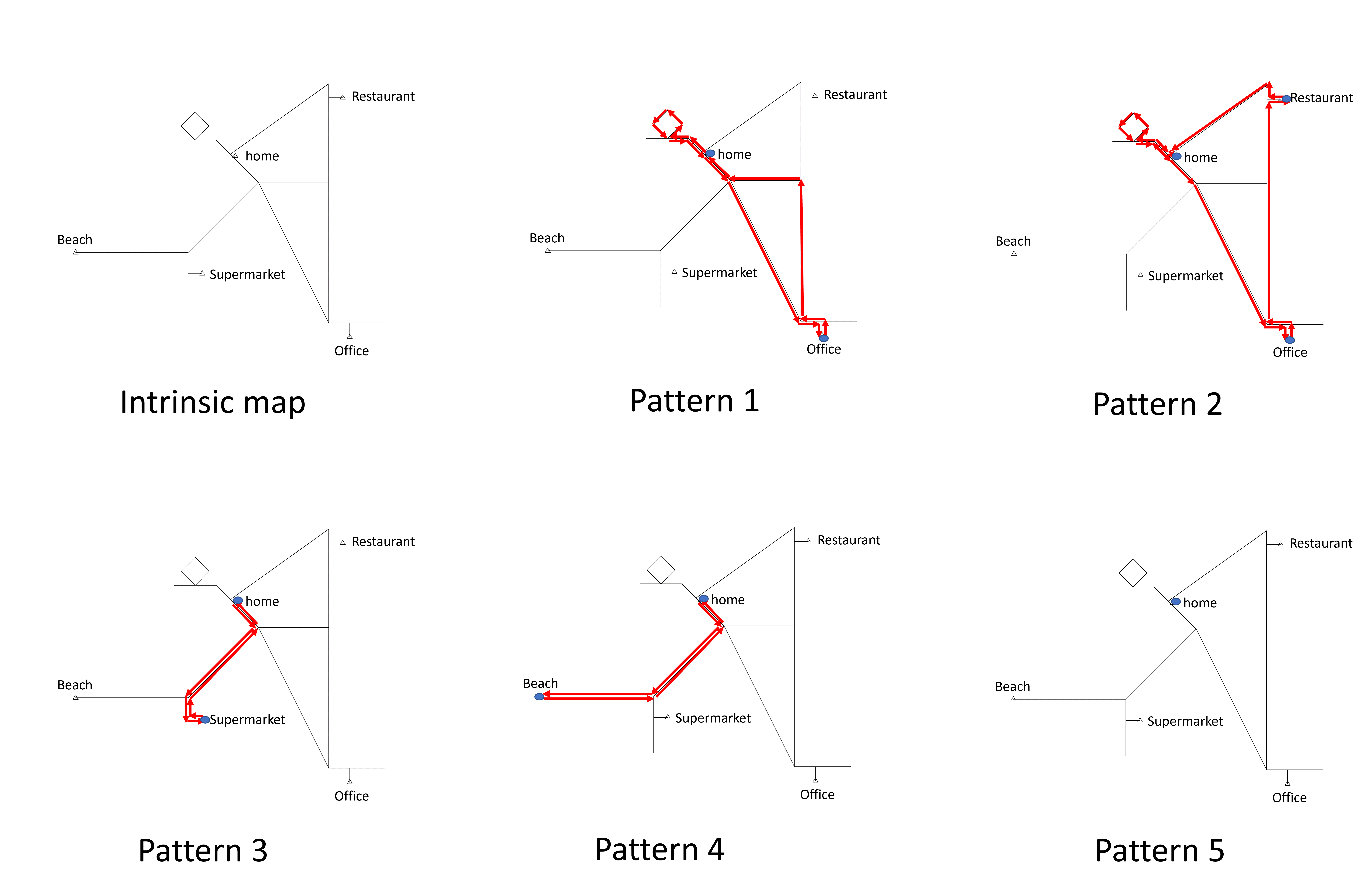
Figure 3 provides an example of the SMM. In this case, there are five possible patterns that the action vector $B$ can be. The first pattern is the following action vector

B=b_{1}=\{\texttt{home},R_{1,1},\texttt{office},R_{1,2},\texttt{home},R_{1,3},\texttt{home}\}.

The road $R_{1,1}$ is from home directly to the office and $R_{1,2}$ is a road from office to home. The road $R_{1,3}$ is where the individual goes to the park in the top region and then goes home without staying. Pattern 3 is the simplest one as it involves only a trip to the local grocery store:

B=b_{3}=\{\texttt{home},R_{31},\texttt{supermarket},R_{3,2},\texttt{home}\}.

The randomness of the action vector $B$ reflects that the individual may follow different activity patterns in a day. Also, even if all the locations $A_{j}$ are the same, the individual may take a different road to move between them. In this construction, we would assume that all possible outcomes of $B$ is a finite set, meaning that the the distribution of $B$ can be described by a probability mass function.

The action vector $B$ only describes the actions (stationary at a location or moving from one to another) of the individual. It does not include any information about the time. Thus, we introduce another random variable $Z$ conditioned on $B$ such that $Z=(Z_{1},\ldots,Z_{2k+1})$ is a random partition of the interval $[0,1]$ such that for $j=1,\ldots,k+1$ , $Z_{2j-1}$ is the amount of time that the individual spend on $A_{j}$ while $Z_{2j}$ is the amount of time that the individual is on the road $R_{j}$ . One can think of $Z$ as a (2k+1)-simplex. When the individual is on the road, we assume that the individual moves between locations with constant velocity. One may use the Dirichlet distribution or truncated Gaussian distribution to generate $Z$ .

To illustrate the idea, we consider again the example in Figure 3. When $B=b_{1}$ , there are a total of $7$ elements in the action vector. So $Z|B=b_{1}$ is a 7-simplex. Suppose $Z=(\frac{9}{24},\frac{1}{24},\frac{8}{24},\frac{1}{24},\frac{2}{24},\frac{1}{24},\frac{2}{24})$ . This means that the individual leaves home at 9 am and spends 1 hour on the road to office. The individual then spends 8 hours in the office and drives home for 1 hour. After a 2-hour stay at home, the individual goes to the park and takes a round trip back home for 1-hour and stays at home for the rest of the day. Note that the vector $Z|B=b_{3}$ will be a 5-simplex since pattern 3 only has 5 possible actions.

Once we have randomly generate $B,Z$ , we can easily obtain the corresponding random trajectory $S(t)$ . Since this model consider a simplified movement of an individual, we call it simple movement model. Although it is a simplified model, it does capture the primary activity of an individual that can be captured by the GPS data. Under SMM, the distribution $P_{S}$ can be characterized by a PMF of $B$ and the PDF of $Z|B$ . Since the action vector $B$ only have finite number of possible outcome, the implied trajectories can be viewed as generating from a mixture model where the action vector $B$ acts as the indicator of the component.

5.1 Recovering anchor locations

In the SMM, we may define the the anchor locations as $\mathcal{A}_{\lambda}=\{a\in\mathcal{A}:P(S(U)=a)>\lambda\}$ for some given threshold $\lambda$ . The threshold $\lambda$ is the proportion of the time that the individual spend at the location $a$ in a day. For instance, the threshold $\lambda=\frac{8}{24}$ should give us the home location as we expect people to spend more than 8 hours in the home in a day. $\lambda=\frac{4}{24}$ may correspond to both the home and the work place.

Suppose that the measurement noise is isotropic Gaussian with variance $\sigma^{2}$ that is known to us, Proposition 2 show that for any $a$ with $P(S(U)=a)\geq\rho_{a},$ we have $f_{GPS}(a)\geq\frac{\rho_{a}}{2\pi\sigma^{2}}.$ This implies that any anchor location $a\in\mathcal{A}_{\lambda}$ will satisfy $f_{GPS}(a)\geq\frac{\lambda}{2\pi\sigma^{2}}.$

Let $\widehat{f}(x)$ be an estimated GPS density, either from the time-weighted approach or the conditional GPS method. We may use the estimated upper level set

\widehat{\mathcal{L}}_{\lambda}=\left\{x:\widehat{f}(x)\geq\frac{\lambda}{2\pi\sigma^{2}}\right\}

(16)

as an estimator for possible locations of $\mathcal{A}_{\lambda}$ . As a result, the level sets of $\widehat{f}(x)$ provide useful information on the anchor locations.

In addition to the level sets, the density local modes of $\widehat{f}(x)$ can be used as an estimator of the anchor locations. Under SMM, anchor locations are where there are probability mass of $S(U)$ . On a regular road $R_{i}$ , there is no probability mass (only a 1D probability density along the road). This property implies that the GPS density $f_{GPS}(x)$ will have local modes around each anchor point (when the measurement noise is not very large). Thus, the local modes within $\widehat{\mathcal{L}}_{\lambda}$ can be used to recover the anchor location:

\widehat{\mathcal{M}}_{\lambda}=\{x\in\widehat{\mathcal{L}}_{\lambda}:\nabla\widehat{f}(x)=0,\,\,\lambda_{1}(\nabla\nabla\widehat{f}(x))<0\},

where $\lambda_{1}(M)$ is the largest eigenvalue of the matrix $M$ and $\nabla\nabla f(x)$ is the Hessian matrix of $f(x)$ .

5.2 Detecting activity spaces

The activity space is a region where the individual spends most of her/his time in a regular day. This region is unique to every individual and can provide key information such as how the built-environment influences the individual (Sherman et al., , 2005). We show how GPS data can be used to determine an individual’s acvity space.

Suppose we know the true GPS density $f_{GPS(x)}$ , a simple approach to quantify the activity space is via the level set indexed by the probability (Polonik, , 1997), also known as the density ranking (Chen and Dobra, , 2020; Chen, , 2019):

	$\displaystyle Q_{\rho}$	$\displaystyle=\min_{\lambda}\left\{\mathcal{L}^{}_{\lambda}:\int_{x\in\mathcal{L}^{}_{\lambda}}f_{GPS}(x)dx\geq\rho\right\}$		(17)
	$\displaystyle\mathcal{L}^{*}_{\lambda}$	$\displaystyle=\left\{x:f_{GPS}(x)\geq\lambda\right\}.$		(17)

Because the level set $\mathcal{L}^{*}_{\lambda}$ are nested when changing $\lambda$ , $Q_{\rho}$ can be recovered by varying $\lambda$ until we have an exactly $\rho$ amount of probability within the level set.

The set $Q_{\rho}$ has a nice interpretation: it is the smallest region where the individual spends at least a proportion of $\rho$ time in it. As a concrete example, $Q_{0.9}$ is where the individual has spent $90\%$ of the time on average. Thus, $Q_{\rho}$ can be used as statistical entity of the activity space. Interestingly, $Q_{\rho}$ can also be interpreted as a prediction region of the individual.

5.2.1 Estimating the activity space

Estimating $Q_{\rho}$ from the data can be done easily by the plug-in estimator approach. A straightforward idea is to use

\displaystyle\widehat{Q}^{*}_{\rho}

\displaystyle=\min_{\lambda}\left\{\widehat{\mathcal{L}}^{*}_{\lambda}:\int_{x\in\widehat{\mathcal{L}}^{*}_{\lambda}}\widehat{f}(x)dx\geq\rho\right\},\qquad\widehat{\mathcal{L}}^{*}_{\lambda}

\displaystyle=\left\{x:\widehat{f}(x)\geq\lambda\right\}.

While this estimator is valid, it may be expansive to compute it because of the integral in the estimator.

Here is an alternative approach to estimating $Q_{\rho}$ without the evaluation of the integral. First, the integral $f_{GPS}(x)dx=dF_{GPS}(x)$ , where $F_{GPS}(x)=P(X(U)+\epsilon\leq x)$ is the corresponding CDF of $f_{GPS}$ . When the timestamps are even-spacing, $F_{GPS}$ can be estimated by the empirical distribution of $X_{i,j}$ . When the timestamps are not even-spacing, we can simply weight each observation by the idea of time-weighting estimator. In more details, a time-weighted estimator of $F_{GPS}$ is

\widehat{F}_{w}(x)=\frac{1}{n}\sum_{i=1}^{n}\sum_{j=1}^{m_{i}}W^{\dagger}_{i,j}I(X_{i,j}\leq x),

where $W^{\dagger}_{i,j}=\frac{t_{i,j+1}-t_{i,j-1}}{2T_{i}},$ if we are using $\widehat{f}_{w}$ and

\qquad W^{\dagger}_{i,j}=\int_{0}^{1}\frac{K_{T}\left(\frac{d_{T}(t_{i,j},t)}{h_{T}}\right)}{\sum_{i^{\prime}=1}^{n}\frac{1}{m_{i^{\prime}}}\sum_{j^{\prime}=1}^{m_{i^{\prime}}}K_{T}\left(\frac{d_{T}(t_{i^{\prime},j^{\prime}},t)}{h_{T}}\right)}dt

if we are using $\widehat{f}_{c}$ . $\widehat{F}_{w}(x)$ can be viewed as a time-weighted EDF. A feature of $\widehat{F}_{w}(x)$ is that when integrating over any region $A$ , we have

\int I(x\in A)d\widehat{F}_{w}(x)=\frac{1}{n}\sum_{i=1}^{n}\sum_{j=1}^{m_{i}}W^{\dagger}_{i,j}I(X_{i,j}\in A).

It is the time-weighted proportion of $X_{i,j}$ inside the region $A$ . With this, we obtain the estimator

	$\displaystyle\widehat{Q}_{\rho}$	$\displaystyle=\min_{\lambda}\left\{\widehat{\mathcal{L}}^{}_{\lambda}:\frac{1}{n}\sum_{i=1}^{n}\sum_{j=1}^{m_{i}}W^{\dagger}_{i,j}I(X_{i,j}\in\widehat{\mathcal{L}}^{}_{\lambda})\geq\rho\right\},$		(18)
	$\displaystyle\widehat{\mathcal{L}}^{*}_{\lambda}$	$\displaystyle=\left\{x:\widehat{f}(x)\geq\lambda\right\};$		(18)

note that $\widehat{f}$ can be either $\widehat{f}_{c}$ or $\widehat{f}_{w}$ . We provide a fast numerical method for computing $\widehat{Q}_{\rho}$ in Appendix A.2.

5.3 Clustering of trajectories

In the SMM, the action vector $B$ is assumed to take a finite number of possible outcomes. While the actual time of each movement under this model may vary a bit according to the random vector $Z$ , resulting in a slightly different trajectory with the same $B$ , the main structure of the trajectory remain similar. This implies that the individual’s trajectories can be clustered into groups according to the action vector $B$ .

While we do not directly observe $B$ , we may use the estimated GPS densities at each day as a noisy representation of $B$ and cluster different days according to the estimated GPS densities.

Here we describe a simple approach to cluster trajectories. Let

\widehat{f}_{c,i}(x)=\frac{1}{nh^{2}}\sum_{j=1}^{m_{i}}\widetilde{W}_{i,j}\cdot K\left(\frac{X_{i,j}-x}{h}\right)

be the estimated time-weighted GPS density of day $i$ , where $\widetilde{W}_{i,j}$ is defined in equation (8). While we may use the pairwise distance matrix among different days $\int(\widehat{f}_{w,a}(x)-\widehat{f}_{w,b}(x))^{2}dx$ as a distance measure, we recommend using a scaled log-density, i.e.,

D_{a,b}=\int\left[\log(\widehat{f}_{c,a}(x)+\xi)-\log(\widehat{f}_{c,b}(x)+\xi)\right]^{2}dx,

(19)

for some small constant $\xi$ to stabilize the log-density. Our empirical studies find that equation (19) works much better in practice because the GPS density is often very skew due to the fact that when the individual is not moving, the density is highly concentrated at a location.

With the distance matrix $D$ , we can perform cluster analysis based on hierarchical cluster or spectral clustering (Von Luxburg, , 2007) to obtain a cluster label for every day. We may also detect outlier activity by examining the distance matrix.

5.3.1 Recovering dynamics after clustering

Once we have done clustering of the data, we obtain a label $G_{i}$ for every day, indicating what cluster the day belongs to. In SMM, trajectories in the same cluster are likely to be from the same action vector $B$ . If we focus on the data of a cluster, we may perform inference on anchor locations or activity space (Sections 5.1 and 5.2) specifically for the corresponding action vector.

Under SMM, trajectories in the same cluster are likely to have the same action vector $B$ (but different temporal distribution $Z$ ). We will expect that the conditional density on the days from the same clusters to be similar. The average behavior of these conditional densities in the same cluster provides us useful information about the latent action vector.

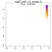
Let $G_{i}\in\{1,\ldots,M\}$ for every $i=1,\ldots,n$ be the cluster label. For a cluster $g\in\{1,\ldots,M\}$ , we compute the cluster conditional GPS density

\widehat{f}_{g}(x|t)=\frac{\sum_{i:G_{i}=g}\frac{1}{m_{i}}\sum_{j=1}^{m_{i}}K\left(\frac{X_{i,j}-x}{h_{X}}\right)K_{T}\left(\frac{d_{T}(t_{i,j},t)}{h_{T}}\right)}{h_{X}^{2}\sum_{i^{\prime}:G_{i^{\prime}}=g}\frac{1}{m_{i^{\prime}}}\sum_{j^{\prime}=1}^{m_{i^{\prime}}}K_{T}\left(\frac{d_{T}(t_{i^{\prime},j^{\prime}},t)}{h_{T}}\right)}.

(20)

How the conditional distribution $\widehat{f}_{g}(x|t)$ changes over time $t$ informs us the movement of this individual under this action vector.

Estimating the conditional center. Since trajectories in the same cluster are similar, we expect the cluster conditional GPS density $\widehat{f}_{g}(x|t)$ to be uni-modal and the mean of this density will be a good representation of its center. Thus, a simple way to track how this distribution moves over time is to study the movement of the mean location, which can be written as

\widehat{\mu}_{g}(t)=\frac{\sum_{i:G_{i}=g}\frac{1}{m_{i}}\sum_{j=1}^{m_{i}}X_{i,j}K_{T}\left(\frac{d_{T}(t_{i,j},t)}{h_{T}}\right)}{\sum_{i^{\prime}:G_{i^{\prime}}=g}\frac{1}{m_{i^{\prime}}}\sum_{j^{\prime}=1}^{m_{i^{\prime}}}K_{T}\left(\frac{d_{T}(t_{i^{\prime},j^{\prime}},t)}{h_{T}}\right)}\in\mbox{$\mathbb{R}$}^{2}.

(21)

Note that this is like a kernel regression with two ‘outcome variables’ (coordinates). For two time points $t_{1}<t_{2}$ , the difference in the center $\widehat{\mu}_{g}(t_{2})-\widehat{\mu}_{g}(t_{1})$ can be interpreted as the average movement in the distribution $\widehat{f}_{g}(x|t)$ within the time interval $[t_{1},t_{2}]$ . Thus, the function $\widehat{\mu}_{g}(t)$ describes the overall dynamics of the trajectories. Note that we may use a local polynomial regression method (Fan, , 2018) to estimate the velocity as well.

6 Real data analysis

We analyze GPS data recorded for a single individual from a longitudinal study of exposure to a cognitive-impairing substance. Participants in this study have been recruited from several cities in a major metropolitan area in the US. The survey data collected comprise one month of GPS tracking with a GPS-enabled smartphone carried by each study participant. The protocol of the study required that the smartphones recorded point locations (latitude, longitude, timestamp) on the spatiotemporal trajectories followed by study participants every minute using a commercially available software. The study participant whose GPS locations are used to illustrate our proposed methodology has been selected at random from the study cohort which comprises more than 150 individuals with complete survey data. In order to preserve any disclosure of private, sensitive information related to this study participant, the latitude and longitude coordinates have been shifted and scaled. The timestamps have been mapped to the unit interval.

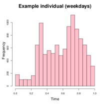
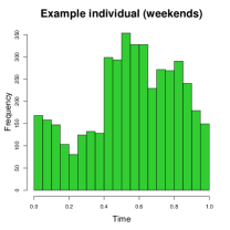
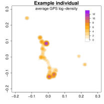
The GPS data for the selected example individual consists of a total of 14,972 observations recorded over $n=30$ days, averaging approximately $m=500$ observations per day. Although the study protocol specified that a new GPS observation should be recorded every minute, the actual recorded timestamps are not regularly distributed over the entire observation window, as illustrated in the first two panels of Figure 4. Consequently, a naive estimation approach would be biased, so we should use either $\widehat{f}_{w}$ or $\widehat{f}_{c}$ for density estimation. We choose $\widehat{f}_{c}$ because it allows for conditional density estimation at any given time. The smoothing bandwidths are set to $h_{X}=0.005$ (longitude/latitude degrees) and $h_{T}=0.02$ (approximately 30 minutes). The third panel in Figure 4 displays the GPS log-density $\log(\widehat{f}_{c}(x)+1)$ . Several high-density regions emerge, suggesting potential anchor locations for the individual.

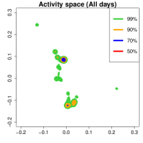
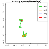
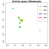
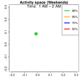
Activity space analysis. Figure 5 presents the individual’s activity space under three scenarios: all days, weekdays, and weekends. The contour region $Q_{\rho}$ represents the area where the individual spends $\rho$ proportion of their time. For instance, $Q_{0.99}$ (green) covers 99% of their time. More than 50% of the time is spent at home, as it includes nighttime. On weekdays (middle panel), 90% of the activities (orange contour) are concentrated at home or the office. To further analyze mobility, we separate the data into weekdays and weekends and examine hourly density variations.

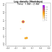
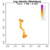
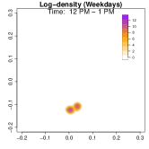
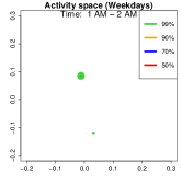
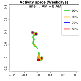
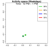
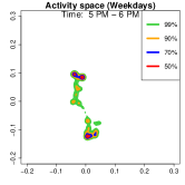
Analysis on the weekdays patterns. Weekday Patterns Figure 6 depicts GPS density distributions across four weekday time windows: 1-2 AM (sleep time), 7-8 AM (morning rush hour), 12-1 PM (noon), and 5-6 PM (evening rush hour). The top row shows the logarithm of the hourly GPS density to mitigate skewness. The bottom row presents the activity space contours for 99% (green), 90% (orange), 70% (blue), and 50% (red) of the time. From Figure 6, we identify five likely anchor locations: one main living place (highest density region in first column) and other two close locations the person may also visit at night (two high-density regions at bottom in the first column) and two office locations (identified in the third panel as high-density regions during midday). By further cluster analysis, we find that there is a main living location (corresponding to the highest density region at night), and an alternative living place close to a park that the example individual sometimes walks inside. The second and fourth columns capture rush-hour mobility, illustrating connectivity between anchor locations.

Figure 6: The hourly GPS log-density and activity space of the example individual during the weekdays. Top row displays the logarithm of the GPS density and the bottom row shows the corresponding activity space of

99\%

(green),

90\%

(orange),

70\%

(blue), and

50\%

(red) average time. We display the interval-specific GPS density of the individual during 1-2 AM (sleep time), 7-8 AM (morning rush hour), 12-1 PM (workplace/school), and 5-6 PM (evening rush hour).

Figure 7: The hourly GPS log-density and activity space of the example individual during the weekends.

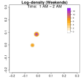
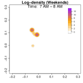
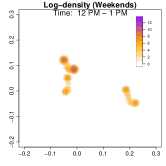
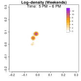
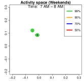
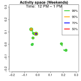
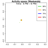
Analysis on the weekends patterns. Figure 7 shows the GPS density during weekends, revealing distinct mobility patterns compared to weekdays. Notably, the office locations (bottom two spots in the third column of Figure 6) show no density. Additional high-density spots appear, likely representing leisure locations (e.g., parks, malls, or beaches). The fourth column indicates a frequent weekend location near home, which is a plaza containing some restaurants and shops. Comparing Figures 6 and 7, we observe a more dispersed mobility pattern on weekends, with multiple high-density regions, whereas weekdays exhibit a concentrated movement pattern, consistent with regular commuting behavior.

Cluster Analysis on Weekday Mobility.

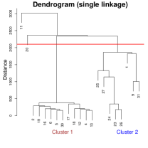
Given the structured weekday patterns, we conduct a cluster analysis to further investigate mobility trends. The results are presented in Figure 8. For each day, we use the same smoothing bandwidths ( $h_{X}$ and $h_{T}$ ) and compute pairwise distances via the integrated squared difference between log-densities:

D_{ij}=\int\left[\log(\widehat{f}_{c,i}(x)+1)-\log(\widehat{f}_{c,j}(x)+1)\right]^{2}dx.

Applying single-linkage hierarchical clustering, the dendrogram (first panel of Figure 8) identifies four clusters, separated by the red horizontal line. Cluster 3 contains Day 11 exclusively. All GPS records on Day 11 are located at home, which corresponds to a wildfire event in the individual’s region that forced he or she to remain indoors throughout the day. So we classify it as an outlier. And cluster 4 also consists of one day (Day 20). On this day, the individual made an additional stop when going back home from office, visiting an entertainment venue that was only recorded once in the entire dataset.

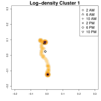
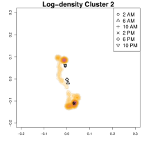
We focus on clusters 1 and 2, comparing their average GPS densities and conditional centers at six different time points. Although both clusters represent commuting patterns, they exhibit distinct anchor locations around the workplace and different evening behaviors. In the lower part of the second and third panels of Figure 8, Cluster 1 shows two high-density regions in the evening, primarily at home and near the office, whereas Cluster 2 contains additional high-density area representing an alternative place to stay overnight (to the right of the main office location) and a park nearby. In particular, on days in Cluster 2, the individual sometimes stays in an alternative home overnight after leaving office rather than returning to the primary home, or visits the park, in the evening (e.g., for a walk) after staying in the alternative home for about 2 hours (and then goes back to the alternative home after visiting the park) By contrast, in Cluster 1, the individual tends to commute directly between home and office without these additional stops.

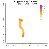
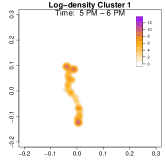
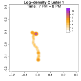
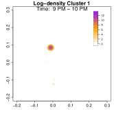
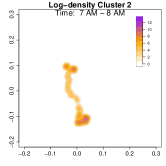
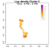
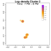
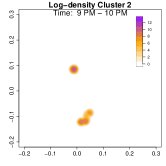
To highlight these differences, Figure 9 compares log-density estimates for four specific time intervals: 7-8 AM (morning rush hour), 5-6 PM (evening rush hour), 7-8 PM (post-work activities), and 9-10 PM (late evening). The top row (Cluster 1) exhibits only 2 high-density regions in the evening, while the bottom row (Cluster 2) shows 4 high-density regions (home, office, park and alternative apartment). As a result, Cluster 2’s pattern emphasizes extended or alternative routines after work including returning to the alternative home or a visit to the park near the work place. The clustering analysis uncovers two distinct weekday mobility patterns: Cluster 1: The individual commutes directly between home and office. Cluster 2: The individual has two options after working: the individual goes back home, otherwise, the individual goes back to the alternative home (sometimes also containing the visit to park after working). This method effectively reveals hidden mobility structures in the data, demonstrating the utility of GPS density estimation in understanding individual movement behavior.

Figure 9: A comparison of the log-density between the two clusters at four specific time intervals: 7-8 AM, 5-6 PM, 7-8 PM, and 9-10 PM. In the morning rush hour, the two clusters show a similar pattern. In the evening time (second to the last columns), the two cluster show significantly different patterns.

7 Discussion and future directions

In this paper, we introduced a statistical framework for analyzing GPS data. The general framework presented in Section 2 applies to GPS data collected from various entities, extending beyond human mobility. For studying human activity patterns, we developed the SMM in Section 5. Despite its simplicity, the SMM effectively captures major movement patterns within a single day and enables meaningful analyses. Our framework lays the foundation for numerous future research directions.

Population study. While this paper primarily focuses on analyzing the activity patterns of a single individual, extending our framework to a population-level analysis remains an open challenge. One key difficulty lies in the variation of anchor locations across individuals, as each person has distinct home and workplace locations. To accommodate population-level studies, modifications to the SMM are necessary to generalize anchor locations and account for heterogeneous mobility patterns. Also, a population-level study will lead to an additional asymptotic regime where the number of individual increases. Together with the two asymptotic regimes of the current framework (number of days and temporal resolution), we encounter a scenario with three asymptotics. The convergence rate and choice of tuning parameters will require adjustments.

Connections to functional data. Our framework transforms GPS data into a density map, establishing interesting connections with functional data analysis (Ramsay and Silverman, , 2002; Wang et al., , 2016). In particular, the daily average GPS density $\widehat{f}_{GPS,i}$ for an individual can be viewed as independent and identically distributed (IID) 2D functional data under the assumption that timestamps are generated in an IID setting. Existing functional data analysis techniques may therefore be applicable, offering new perspectives on GPS-based modeling. Notably, methods introduced in Section 5 suggest potential links between structural assumptions in the SMM and those in functional data analysis. In addition, when the sampling frequency is high, the two coordinates in the GPS data can be separated viewed as two functional data with a common but irregular spacing (Gervini, , 2009). Under this point of view, we may directly apply methods from functional data to handle GPS data. This alternative perspective may lead to a different framework for analyzing GPS data. Further exploration of these connections is an important research direction.

Limiting regime of measurement errors. Our current analysis considers asymptotic limits where the number of days $n\rightarrow\infty$ and the temporal resolution $|t_{i,j}-t_{i,j+1}|\rightarrow 0$ . Another intriguing limit involves the measurement noise level, where $\mbox{$\mathbb{E}$}(\|\epsilon\|^{2})\rightarrow 0$ , reflecting advancements in GPS technology. However, as measurement errors vanish, the density function $f_{GPS}$ becomes ill-defined. In this noiseless scenario, the distribution of a random trajectory point $X^{*}=X(U)$ consists of a mixture of point masses (at anchor locations) and 1D distributions representing movement along trajectories. Addressing the challenges posed by singular measures (Chen and Dobra, , 2020; Chen, , 2019) in this regime is a crucial area for future investigation.

Alternative random trajectory models. While the SMM proposed in Section 5 provides practical utility and meaningful insights, it does not precisely model an individual’s movement. Specifically, the SMM assumes a constant velocity when an individual is in motion, leading to a step-function velocity profile with abrupt jumps at transitions between movement and stationary states. This assumption deviates from realistic human mobility patterns. Developing more sophisticated models that accurately capture velocity dynamics and movement variability remains an open problem for future research.

Topological data analysis. Topological data analysis (TDA; Wasserman, 2018; Chazal and Michel, 2021) is a data analysis technique to study the shape of features inside data. A common application of TDA is to study the morphology of the probability density function. The TDA can be applied to analyze GPS data in two possible ways. The first application is to use TDA to analyze the morphology of GPS density functions. This allows us to further understand the activity space. The second applications is to use TDA to investigate the latent trajectories generated the GPS data. The common/persistent features of trajectories informs us important characteristics of the individual’s activity patterns.

References

Andrade and Gama, (2020) Andrade, T. and Gama, J. (2020). Identifying points of interest and similar individuals from raw gps data. In Mobility Internet of Things 2018: Mobility IoT, pages 293–305. Springer.
Barnett and Onnela, (2020) Barnett, I. and Onnela, J.-P. (2020). Inferring mobility measures from gps traces with missing data. Biostatistics, 21(2):e98–e112.
Burzacchi et al., (2024) Burzacchi, A., Bellanger, L., Gall, K. L., Stamm, A., and Vantini, S. (2024). Generating synthetic functional data for privacy-preserving gps trajectories. arXiv preprint arXiv:2410.12514.
Cadre, (2006) Cadre, B. (2006). Kernel estimation of density level sets. Journal of multivariate analysis, 97(4):999–1023.
Chabert-Liddell et al., (2023) Chabert-Liddell, S.-C., Bez, N., Gloaguen, P., Donnet, S., and Mahévas, S. (2023). Auto-encoding gps data to reveal individual and collective behaviour.
Chacón, (2015) Chacón, J. E. (2015). A population background for nonparametric density-based clustering. Statistical Science, 30(4):518–532.
Chacón and Duong, (2018) Chacón, J. E. and Duong, T. (2018). Multivariate kernel smoothing and its applications. Chapman and Hall/CRC.
Chacón et al., (2011) Chacón, J. E., Duong, T., and Wand, M. P. (2011). Asymptotics for general multivariate kernel density derivative estimators. Statistica Sinica, 21(2):807–840. Accessed 5 Mar. 2025.
Chazal and Michel, (2021) Chazal, F. and Michel, B. (2021). An introduction to topological data analysis: fundamental and practical aspects for data scientists. Frontiers in artificial intelligence, 4:667963.
Chen, (2019) Chen, Y.-C. (2019). Generalized cluster trees and singular measures. The Annals of Statistics, 47(4):2174–2203.
Chen and Dobra, (2020) Chen, Y.-C. and Dobra, A. (2020). Measuring human activity spaces from GPS data with density ranking and summary curves. The Annals of Applied Statistics, 14(1):409 – 432.
Chen et al., (2017) Chen, Y.-C., Genovese, C. R., and Wasserman, L. (2017). Density level sets: Asymptotics, inference, and visualization. Journal of the American Statistical Association, 112(520):1684–1696.
Duong, (2024) Duong, T. (2024). Using iterated local alignment to aggregate trajectory data into a traffic flow map. arXiv preprint arXiv:2406.17500.
Early and Sykulski, (2020) Early, J. J. and Sykulski, A. M. (2020). Smoothing and interpolating noisy gps data with smoothing splines. Journal of Atmospheric and Oceanic Technology, 37(3):449–465.
Elmasri et al., (2023) Elmasri, M., Labbe, A., Larocque, D., and Charlin, L. (2023). Predictive inference for travel time on transportation networks. The Annals of Applied Statistics, 17(4):2796–2820.
Fan, (2018) Fan, J. (2018). Local polynomial modelling and its applications: monographs on statistics and applied probability 66. Routledge.
Gervini, (2009) Gervini, D. (2009). Detecting and handling outlying trajectories in irregularly sampled functional datasets. The Annals of Applied Statistics, pages 1758–1775.
Hägerstrand, (1963) Hägerstrand, T. (1963). Geographic measurements of migration. In Sutter, J., editor, Human Displacements: Measurement Methodological Aspects. Monaco.
Hägerstrand, (1970) Hägerstrand, T. (1970). What about people in regional science? Papers of the Regional Science Association, 24:7–21.
Huang et al., (2023) Huang, Y., Abdelhalim, A., Stewart, A., Zhao, J., and Koutsopoulos, H. (2023). Reconstructing transit vehicle trajectory using high-resolution gps data. In 2023 IEEE 26th International Conference on Intelligent Transportation Systems (ITSC), pages 5247–5253. IEEE.
Ley and Verdebout, (2017) Ley, C. and Verdebout, T. (2017). Modern directional statistics. Chapman and Hall/CRC.
Mao et al., (2023) Mao, J., Liu, L., Huang, H., Lu, W., Yang, K., Tang, T., and Shi, H. (2023). On the temporal-spatial analysis of estimating urban traffic patterns via gps trace data of car-hailing vehicles. arXiv preprint arXiv:2306.07456.
Mardia and Jupp, (2009) Mardia, K. V. and Jupp, P. E. (2009). Directional statistics. John Wiley & Sons.
Meilán-Vila et al., (2021) Meilán-Vila, A., Francisco-Fernández, M., Crujeiras, R. M., and Panzera, A. (2021). Nonparametric multiple regression estimation for circular response. TEST, 30(3):650–672.
Newson and Krumm, (2009) Newson, P. and Krumm, J. (2009). Hidden markov map matching through noise and sparseness. In 17th ACM SIGSPATIAL International Conference on Advances in Geographic Information Systems (ACM SIGSPATIAL GIS 2009), November 4-6, Seattle, WA, pages 336–343.
Nguyen et al., (2023) Nguyen, T. D., Pham Ngoc, T. M., and Rivoirard, V. (2023). Adaptive warped kernel estimation for nonparametric regression with circular responses. Electronic Journal of Statistics, 17(2):4011–4048.
Papoutsis et al., (2021) Papoutsis, P., Fennia, S., Bridon, C., and Duong, T. (2021). Relaxing door-to-door matching reduces passenger waiting times: A workflow for the analysis of driver gps traces in a stochastic carpooling service. Transportation Engineering, 4:100061.
Pewsey and García-Portugués, (2021) Pewsey, A. and García-Portugués, E. (2021). Recent advances in directional statistics. Test, 30(1):1–58.
Polonik, (1997) Polonik, W. (1997). Minimum volume sets and generalized quantile processes. Stochastic processes and their applications, 69(1):1–24.
Ramsay and Silverman, (2002) Ramsay, J. O. and Silverman, B. W. (2002). Applied functional data analysis: methods and case studies. Springer.
Schönfelder and Axhausen, (2004) Schönfelder, S. and Axhausen, K. W. (2004). On the variability of human activity spaces. In Koll-Schretzenmayr, M., Keiner, M., and Nussbaumer, G., editors, The Real and Virtual Worlds of Spatial Planning, pages 237–262. Springer Verlag, Berlin, Heidelberg.
Scott, (2015) Scott, D. W. (2015). Multivariate density estimation: theory, practice, and visualization. John Wiley & Sons.
Sherman et al., (2005) Sherman, J. E., Spencer, J., Preisser, J. S., Gesler, W. M., and Arcury, T. A. (2005). A suite of methods for representing activity space in a healthcare accessibility study. International Journal of Health Geographics, 4:24–24.
Silverman, (2018) Silverman, B. W. (2018). Density estimation for statistics and data analysis. Routledge.
Simon, (2014) Simon, L. (2014). Introduction to Geometric Measure Theory. Cambridge University Press.
Tsybakov, (1997) Tsybakov, A. B. (1997). On nonparametric estimation of density level sets. The Annals of Statistics, 25(3):948–969.
Von Luxburg, (2007) Von Luxburg, U. (2007). A tutorial on spectral clustering. Statistics and computing, 17:395–416.
Wang et al., (2016) Wang, J.-L., Chiou, J.-M., and Müller, H.-G. (2016). Functional data analysis. Annual Review of Statistics and its application, 3(1):257–295.
Wasserman, (2006) Wasserman, L. (2006). All of nonparametric statistics. Springer Science & Business Media.
Wasserman, (2018) Wasserman, L. (2018). Topological data analysis. Annual Review of Statistics and Its Application, 5(1):501–532.
Yang et al., (2022) Yang, Y., Jia, B., Yan, X.-Y., Li, J., Yang, Z., and Gao, Z. (2022). Identifying intercity freight trip ends of heavy trucks from gps data. Transportation Research Part E: Logistics and Transportation Review, 157:102590.

SUPPLEMENTARY MATERIAL

Numerical techniques (Section A):: We provide some useful numerical techniques for computing our estimators.
Simulations (Section B):: We provide a simulation study to investigate the performance of our method.
Assumptions (Section C):: All technical assumptions for the asymptotic theory are included in this section.
Proofs (Section D):: The proofs of the theoretical results are given in this section.
Data and R scripts:: See the online supplementary file.

Appendix A Numerical techniques

A.1 Conditional estimator as a weighted estimator

Recall that the estimator $\widehat{f}_{c}(x)$ in equation (8) is

	$\displaystyle\widehat{f}_{c}(x)=\int_{0}^{1}\widehat{f}(x\|t)dt$	$\displaystyle=\frac{1}{nh^{2}}\sum_{i=1}^{n}\sum_{j=1}^{m_{i}}\widetilde{W}_{i,j}\cdot K\left(\frac{X_{i,j}-x}{h}\right),$
	$\displaystyle\widetilde{W}_{i,j}$	$\displaystyle=n\cdot\int_{0}^{1}\frac{K_{T}\left(\frac{d_{T}(t_{i,j},t)}{h_{T}}\right)}{\sum_{i^{\prime}=1}^{n}\frac{1}{m_{i^{\prime}}}\sum_{j^{\prime}=1}^{m_{i^{\prime}}}K_{T}\left(\frac{d_{T}(t_{i^{\prime},j^{\prime}},t)}{h_{T}}\right)}dt$

and the conditional PDF in equation (7),

\widehat{f}(x|t)=\frac{\sum_{i=1}^{n}\frac{1}{m_{i}}\sum_{j=1}^{m_{i}}K\left(\frac{X_{i,j}-x}{h_{X}}\right)K_{T}\left(\frac{d_{T}(t_{i,j},t)}{h_{T}}\right)}{h_{X}^{2}\cdot\sum_{i^{\prime}=1}^{n}\frac{1}{m_{i^{\prime}}}\sum_{j^{\prime}=1}^{m_{i^{\prime}}}K_{T}\left(\frac{d_{T}(t_{i^{\prime},j^{\prime}},t)}{h_{T}}\right)}=\frac{1}{nh^{2}}\sum_{i=1}^{n}\sum_{j=1}^{m_{i}}\omega_{i,j}(t)\cdot K\left(\frac{X_{i,j}-x}{h}\right),

where

\omega_{i,j}(t)=n\cdot\frac{K\left(\frac{X_{i,j}-x}{h_{X}}\right)K_{T}\left(\frac{d_{T}(t_{i,j},t)}{h_{T}}\right)}{\sum_{i^{\prime}=1}^{n}\frac{1}{m_{i^{\prime}}}\sum_{j^{\prime}=1}^{m_{i^{\prime}}}K_{T}\left(\frac{d_{T}(t_{i^{\prime},j^{\prime}},t)}{h_{T}}\right)}.

is a local weight at time $t$ . So both estimators are essentially the weighted 2D KDE with different weights. This allows us to quickly compute the estimator using existing kernel smoothing library such as the ks library in R.

Moreover, the weights are connected by the integral

\widetilde{W}_{i,j}=\int_{0}^{1}\omega_{i,j}(t).

If we are interested in only the time interval $A\subset[0,1]$ , we just need to adjust the weight to be

\widetilde{W}_{A,i,j}=\int_{A}\omega_{i,j}(t)

and rerun the weighted 2D KDE. In practice, we often perform a numerical approximation to the integral based on a dense grid of $[0,1]$ . Computing the weights $\widetilde{W}_{A,i,j}$ can be done easily by using only the grid points inside the interval $A$ .

A.2 A fast algorithm for the activity space

Recall that the $\rho$ -activity space is

	$\displaystyle\widehat{Q}_{\rho}$	$\displaystyle=\min_{\lambda}\left\{\widehat{\mathcal{L}}^{}_{\lambda}:\frac{1}{n}\sum_{i=1}^{n}\sum_{j=1}^{m_{i}}W^{\dagger}_{i,j}I(X_{i,j}\in\widehat{\mathcal{L}}^{}_{\lambda})\geq\rho\right\},$
	$\displaystyle\widehat{\mathcal{L}}^{*}_{\lambda}$	$\displaystyle=\left\{x:\widehat{f}(x)\geq\lambda\right\}.$

Numerically, the minimization in $\widehat{Q}_{\rho}$ is not needed. Since the time-weight EDF $\widehat{F}_{w}(x)$ is a distribution function with a probability mass of $\frac{1}{n}W^{\dagger}_{i,j}$ on $X_{i,j}$ . Therefore, the summation $\frac{1}{n}\sum_{i=1}^{n}\sum_{j=1}^{m_{i}}W^{\dagger}_{i,j}I(X_{i,j}\in\widehat{\mathcal{L}}^{*}_{\lambda})$ remains the same when we vary $\lambda$ without including any observation $X_{i,j}$ . Using this insight, let $\widehat{p}_{i,j}=\widehat{f}(X_{i,j})$ be the estimated density at $X_{i,j}$ . We then ordered all observations (across every day) according to the estimated density evaluated at each point

\widehat{p}_{(1)}<\widehat{p}_{(2)}<\ldots\widehat{p}_{(N_{n})}

and let $(X_{(1)},W^{\dagger}_{(1)}),\ldots,(X_{(N_{n})},W^{\dagger}_{(N_{n})})$ be the corresponding location and weight from $(X_{i,j},W^{\dagger}_{i,j})$ . Note that $N_{n}=\sum_{i=1}^{n}m_{i}$ is total number of observations.

In this way, if we choose $\lambda=p_{(k)}$ , the level set $\widehat{\mathcal{L}}^{*}_{p_{(k)}}$ will cover all observations of indices $(k),(k+2),\ldots,(N_{n})$ , leading to the proportion of $\frac{1}{n}\left(W^{\dagger}_{(k)}+W^{\dagger}_{(k+1)}+\ldots W^{\dagger}_{(N_{n})}\right)$ being covered inside $\widehat{\mathcal{L}}^{*}_{p_{(k)}}$ . Note that the division of $n$ is to account for the summation over $n$ days. As a result, for a given proportion $\rho$ , we only need to find the largest index $k^{*}_{\rho}$ such that the upper cumulative sum of $t_{(k)}$ is above $\rho$ :

k^{*}_{\rho}=\max\left\{k:\frac{1}{n}\sum_{\ell=k}^{N_{n}}W^{\dagger}_{(\ell)}\geq\rho\right\}.

(22)

With this, the choice $\lambda=p_{(k^{*}_{\rho})}$ leads to the set

\widehat{\mathcal{L}}^{*}_{p_{(k^{*}_{\rho})}}=\widehat{Q}_{\rho}.

(23)

Appendix B Simulation

B.1 Design of simulations

Pattern

Probability

Expected duration

(Hours)

\eta

q

Actions

Pattern 1

15/28

0.15

0.5

At home

0.5

0.08

0.25

Home to office

0.15

0.5

At office

0.6

0.08

0.25

Office to home

0.2

0.6

At home

0.06

0.15

Home to park to home

2.9

Home

Pattern 2

5/28

8.5

0.15

0.5

Home

0.5

0.08

0.25

Home to office

0.15

0.5

At office

0.75

0.08

0.25

Office to restaurant

0.08

0.25

At restaurant

0.4

0.08

0.25

Restaurant to home

0.95

0.1

0.3

At home

0.06

0.15

Home to park to home

2.9

At home

Pattern 3

4/28

0.3

At home

0.75

0.15

0.45

Home to supermarket

2.5

0.3

At supermarket

0.75

0.15

0.45

Supermarket to home

At home

Pattern 4

1/28

0.3

At home

0.8

0.3

0.7

Home to beach

5.7

0.35

Beach

0.8

0.3

0.7

Beach to home

6.7

At home

Pattern 5

3/28

At home

Table 1: An SMM model that we use for simulation. Specifically, there are totally five daily activity patterns used for simulation. Each location’s duration follows a truncated normal distribution with mean (Expected Duration), standard deviation

\eta

, and half-width

q

. Times shown are in hours. The final row for each pattern (where

\eta

and

q

are blank) absorbs any remaining time up to 24 hours.

To evaluate the performance of the proposed activity density estimators, we construct a simplified scenario involving a single fictitious individual residing in a small-scale world. This world contains five anchor points: home, office, restaurant, beach, and supermarket connected by several routes (Figure 3, the first panel).

Activity patterns.

We design five distinct daily activity patterns for this individual, illustrated in the 2nd to 6th panel in Figure 3. Specific details including the order of visits, the expected time spent at each location, and the probability of selecting each pattern are summarized in Table 1. Each day, the individual randomly chooses one of these five patterns.

For each location in a chosen pattern, the duration is drawn from a truncated normal distribution:

z_{i}\mid b\sim\mathcal{N}\bigl{(}\mu_{b,i},\,\eta_{b,i}^{2}\bigr{)}\quad\text{truncated to}\quad\bigl{(}\mu_{b,i}-q_{b,i},\;\mu_{b,i}+q_{b,i}\bigr{)},

where $\mu_{b,i}$ and $\eta_{b,i}$ are the mean and standard deviation, and $q_{b,i}\in[0,1]$ sets a reasonable range for the duration. The duration of final location in each pattern is computed as whatever time remains in the 24-hour day once all previous locations have been visited.

There are two reasons we use a truncated Gaussian distribution for the duration of each position:

•

First, controlling variance: By adjusting $\eta_{b,i}$ , we can reflect realistic scenarios; for example, weekday departures from home tend to be less variable than weekend departures for a beach visit. Hence, we set the variance of duration of the first position higher on weekends.
•

Second, ensuring a reasonable time distribution: Truncation avoids unrealistic time of visiting for some places (for example, a restaurant stay should not exceed typical operating hours).

Our ultimate goal is to estimate $f_{GPS}$ and $f_{GPS,A}$ over the time interval $A=\bigl{[}\tfrac{8}{24},\,\tfrac{10}{24}\bigr{]}$ , which corresponds to the morning rush hour between 8 AM and 10 AM.

Timestamp generation. For simplicity, we assume that every day has equal number of observations, i.e., $m_{i}=m$ , and we choose $(n,m)$ as

n\in\{7,30,90\}\quad m\in\{159,479,1439\},

such choice of $n$ reflects one week, one month, and three months of GPS observation data. The choices of $m$ correspond to one observation every 9 minutes, 3 minutes, or 1 minute on average.

To investigate estimator performance under both regular and irregular frequencies of observations, we generate timestamps in two different ways:

1.

Even-spacing: In each simulated day, the $m$ timestamps are evenly spaced at intervals of $\tfrac{1440}{m+1}$ minutes. Then, the GPS observations are recorded every $\frac{1440}{m+1}$ minutes.
2.
Realistic: To generate non-uniform timestamps which align with the realistic recording, We use real GPS data described in Section 6 in the following procedure:
1. (a)
  
  Randomly select one individual from the real dataset.
2. (b)
  
  For each day, randomly choose one day from that individual.
3. (c)
  
  If the chosen day has fewer than $m$ real timestamps, generate the additional timestamps by sampling from a Gaussian kernel density estimate of that day’s timestamp distribution (using Silverman’s rule of thumb for bandwidth). If the chosen day has more than $m$ real timestamps, randomly remove timestamps until $m$ timestamps remain, where the probability of removal for each observation is the same.
This process yields $m$ timestamps per simulated day, preserving the original non-uniformity found in the selected individual’s data. The real data’s timestamp distribution is possibly very skew. This procedure preserves the original day-to-day skew and clustering patterns of timestamps found in real data. Figure 4 illustrates an example of a highly skewed timestamp distribution for one individual.

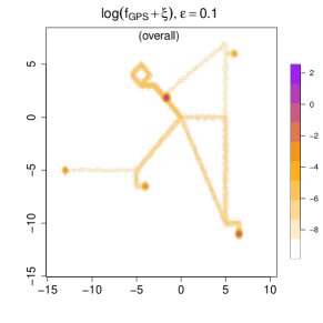
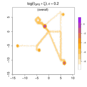
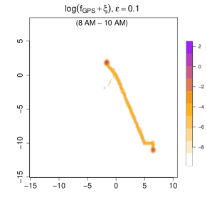
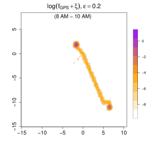
Measurement errors. We introduce measurement errors by drawing from a Gaussian noise distribution with $\sigma=0.1$ or $\sigma=0.2$ . The corresponding $\log(f_{GPS}+\xi)$ is shown in Figure 10, where $\xi$ is set as 0.0001. Note that we use a log-scale because the anchor locations (home and office) have a very high $f_{GPS}$ , which would otherwise dominate the scale so that we cannot see the overall pattern well. In the top panels, we display $\log(f_{GPS}+\xi)$ while in the bottom panel, we focus on the density during the morning rush hour (8 AM to 10 AM).

Compared with the real-data analysis in Section 6, here we choose a smaller $\xi$ . This adjustment is caused by the scale of coordinates. The density value will be lower if the data is in a larger spatial region. This smaller $\xi$ ensures low-frequency or low-duration regions, such as the route between home and the beach, remain distinguishable from truly unvisited areas in both visualization and the further analysis such as clustering. As a result, in subsequent clustering analyses, the reduced $\xi$ value helps more clearly separate visited versus unvisited locations, thereby improving the distinctiveness among different mobility patterns.

Bandwidth selection. After preliminary experiments using mean integrated squared error (MISE) as a performance measure, we found the following reference rule for the spatial and temporal smoothing bandwidth:

h_{X}\;=\;0.065\,\biggl{(}\frac{\sqrt{s_{x,1}^{2}+s_{x,2}^{2}}}{\sum_{i=1}^{n}m_{i}}\,\biggr{)}^{\tfrac{1}{6}},\quad h_{T}=0.05\,\biggl{(}\frac{n}{\sum_{i=1}^{n}m_{i}}\,\biggr{)}^{\tfrac{1}{3}}

where

s_{x,l}\;=\;\sqrt{\sum_{k=1}^{n_{d}}\sum_{i=1}^{m_{k}}w_{i,j}\,\bigl{(}x_{i,j,l}-\mu_{l}\bigr{)}^{2}},l=1,2\quad w_{i,j}\;=\;\frac{t_{i,j+1}-t_{i,j-1}}{2\,n},\quad\mu_{1}\;=\;\sum_{i=1}^{n}\sum_{j=1}^{m_{i}}w_{i,j}\,x_{i,j,l}.

Here, $(x_{i,j,1},x_{i,j,2})$ denotes the spatial coordinates of the $j$ -th observation on day $i$ , and $t_{i,j}$ is its (normalized) timestamp within day $i$ . The weights $w_{k,i}$ ensure proper normalization over the total number of days $n$ and allow for variable sampling rates within a day.

Compared with standard bandwidth heuristics such as Silverman’s rule of thumb for multivariate kernels Chacón et al., (2011), our scale constants are noticeably smaller. This discrepancy arises because Silverman’s rule is often derived under assumptions of (approximately) unimodal or smooth data distributions. In contrast, our simulated environment exhibits strongly localized activity peaks due to prolonged stays at a small number of anchor points (e.g., home and office). As a result, the density near these anchor points is extremely high compared with other regions. A smaller bandwidth helps avoid oversmoothing these sharp peaks, thereby reducing bias and improving local accuracy of the estimated density. From a MISE perspective, capturing these density spikes precisely is critical, since errors around densely occupied points can contribute disproportionately to the integrated error. Consequently, a smaller scale constant not only accommodates the multimodal nature of the data but also minimizes MISE by enhancing resolution in areas with concentrated activity.

B.2 Results on the MISE

Estimating the average GPS density. For each combination of $(n,m)$ , we report the averaged mean integrated squared error (MISE) over a $121\times 99$ grid averaged over 100 repetitions, where each cell has area $0.2\times 0.2$ . The results for estimating $f_{GPS}$ appear in Tables 2–3.

Even-spacing		$\epsilon=0.2$			$\epsilon=0.1$
$n$	$m$	$\widehat{f}_{w}$	$\widehat{f}_{c}$	$\widehat{f}_{naive}$	$\widehat{f}_{w}$	$\widehat{f}_{c}$	$\widehat{f}_{naive}$
7	159	0.0839	0.0812	0.0839	0.8571	0.8482	0.8571
7	479	0.0619	0.0599	0.0619	0.6426	0.6353	0.6426
7	1439	0.0456	0.0438	0.0456	0.4442	0.4375	0.4442
30	159	0.0473	0.045	0.0473	0.5967	0.5874	0.5967
30	479	0.0359	0.0341	0.0359	0.4321	0.4249	0.4321
30	1439	0.0209	0.0197	0.0209	0.268	0.2623	0.268
90	159	0.0368	0.0344	0.0368	0.4592	0.4495	0.4592
90	479	0.0225	0.021	0.0225	0.3109	0.3041	0.3109
90	1439	0.0113	0.0105	0.0113	0.1729	0.1675	0.1729

Table 2: The MISE of the three methods for estimating the daily density during under evenly spacing timestamps.

Realistic		$\epsilon=0.2$			$\epsilon=0.1$
$n$	$m$	$\widehat{f}_{w}$	$\widehat{f}_{c}$	$\widehat{f}_{naive}$	$\widehat{f}_{w}$	$\widehat{f}_{c}$	$\widehat{f}_{naive}$
7	159	0.113	0.0844	0.1457	0.9321	0.8747	1.0424
7	479	0.097	0.0622	0.1192	0.7135	0.6473	0.819
7	1439	0.0925	0.0489	0.1017	0.5616	0.4736	0.642
30	159	0.0708	0.0472	0.0934	0.6512	0.5873	0.7415
30	479	0.0575	0.0325	0.0787	0.4859	0.4143	0.5773
30	1439	0.0462	0.0219	0.0642	0.349	0.2801	0.4359
90	159	0.0562	0.0337	0.0778	0.5228	0.4529	0.6108
90	479	0.0415	0.0224	0.0641	0.3734	0.3119	0.4677
90	1439	0.0286	0.0106	0.0432	0.2358	0.1751	0.3172

Table 3: The MISE of the three methods for estimating the daily density during under realistic timestamp distributions.

In Tables 2 (even-spacing), we see that all methods work well with the conditional method $\widehat{f}_{c}$ that performs slightly better than the others. And the marginal method $\widehat{f}_{w}$ has almost same MISE as naive method $\widehat{f}_{naive}$ . Because timestamps are recorded at uniform intervals, each observation naturally represents a comparable portion of the day, thus reducing the penalty from ignoring time differences. A similar conclusion holds if timestamps are generated uniformly in $[0,1]$ .

In contrast, when timestamps are drawn from the real dataset, the results change significantly. Real-world GPS records are often non-uniform in time, so the naive estimator which assumes each data point is equally representative suffers from a pronounced bias. This effect is especially evident in the last row of Table 3, where $\widehat{f}_{\mathrm{naive}}$ exhibits a substantially higher MISE than either of the proposed estimators. Notably, both $\widehat{f}_{w}$ and $\widehat{f}_{c}$ handle irregular sampling much more effectively, resulting in significantly lower MISE.

Estimating the interval-specific GPS density. In addition to the average GPS densities, we also consider the case of estimating the GPS density during the morning rush hour $A=[\frac{8}{24},\frac{10}{24}]$ (8 AM - 10 AM). Tables 4 and 5 present the results for this interval-specific density.

The performance trends mirror those observed for daily averages (Table 4): all three estimators remain consistent, and the conditional method $\widehat{f}_{c}$ has a slight edge over the other two. The naive and weighted methods $\widehat{f}_{w}$ show comparable MISE values.

Table 5 shows the MISE of three estimators when we generate the timestamps from a realistic distribution. As with the daily density estimation, the real (irregular) distribution of timestamps reveals a clear advantage for $\widehat{f}_{c}$ . The naive approach again shows higher MISE, though in this specific morning interval, the difference between $\widehat{f}_{w}$ and $\widehat{f}_{\mathrm{naive}}$ is smaller than in the full-day scenario. This arises because the distribution of the real data timestamps between 8 AM and 10 AM are not as severely skewed as the distribution of timestamps in the whole day, so the advantage of $\widehat{f}_{w}$ is somewhat diminished.

Overall, the results confirm that both $\widehat{f}_{w}$ and $\widehat{f}_{c}$ more robustly handle uneven timestamp distributions compared to the naive approach, and that $\widehat{f}_{c}$ typically offers the best performance in terms of MISE across a variety of sampling settings.

Realistic		$\epsilon=0.2$			$\epsilon=0.1$
$n$	$m$	$\widehat{f}_{w}$	$\widehat{f}_{c}$	$\widehat{f}_{naive}$	$\widehat{f}_{w}$	$\widehat{f}_{c}$	$\widehat{f}_{naive}$
7	159	0.1802	0.1212	0.1794	1.2959	0.8483	1.2935
7	479	0.1287	0.0917	0.1281	0.9944	0.6345	0.9922
7	1439	0.1184	0.0789	0.1184	0.8261	0.4762	0.8253
30	159	0.0971	0.0676	0.0964	0.864	0.5967	0.8615
30	479	0.0787	0.0548	0.0783	0.6974	0.436	0.6955
30	1439	0.0498	0.0333	0.0497	0.4488	0.2693	0.4482
90	159	0.0777	0.0545	0.0772	0.7083	0.4752	0.7058
90	479	0.049	0.0341	0.0489	0.4616	0.3144	0.46
90	1439	0.038	0.0204	0.0379	0.3093	0.1817	0.3089

Table 4: The MISE of the three methods for estimating the density during the rush hour (8-10 AM) under evenly spacing timestamps.

Realistic		$\epsilon=0.2$			$\epsilon=0.1$
$n$	$m$	$\widehat{f}_{w}$	$\widehat{f}_{c}$	$\widehat{f}_{naive}$	$\widehat{f}_{w}$	$\widehat{f}_{c}$	$\widehat{f}_{naive}$
7	159	0.1489	0.1099	0.1522	1.0886	0.816	1.1085
7	479	0.1064	0.0812	0.1123	0.8289	0.582	0.8495
7	1439	0.0909	0.0749	0.1006	0.6751	0.4664	0.7054
30	159	0.0894	0.065	0.0902	0.7808	0.5702	0.7857
30	479	0.0637	0.0463	0.0651	0.5714	0.3954	0.5776
30	1439	0.0542	0.0424	0.0573	0.4103	0.3121	0.4225
90	159	0.0616	0.0482	0.0627	0.5631	0.4508	0.568
90	479	0.046	0.0357	0.0486	0.3906	0.3136	0.4013
90	1439	0.0286	0.0162	0.0304	0.2301	0.1587	0.2373

Table 5: The MISE of the three methods for estimating the density during the rush hour (8-10 AM) under the realistic timestamp distribution.

B.3 Applications based on the simple movement model

In our simulation setup, Pattern 1 and Pattern 2 correspond to typical weekday schedules (containing the office as an anchor point), whereas Pattern 3, Pattern 4, and Pattern 5 represent potential weekend routines (not containing office as anchor point). We separately analyze the data in weekdays and weekends using the framework of Section 5. Throughout this subsection, we fix the measurement error at $\sigma=0.2$ and assume evenly spaced timestamps with 479 GPS observations per day. We generate a total of 90 simulated days under these conditions.

B.3.1 Anchor location recovering

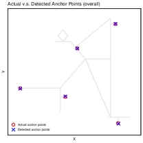
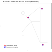
From Table 1, we identify three anchor locations for weekdays (home, office, restaurant) and another set of three for weekends (home, supermarket, beach). Across the entire 90 days, these yield five un anchor points overall.

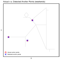
Using the method described in Section 5.1 with $\lambda=0.0055$ , we recover all anchor locations accurately, whether we consider:

1. All 90 days combined,

2. Weekdays only (Patterns 1 and 2), or

3. Weekends only (Patterns 3, 4, and 5).

Figure 11 compares the true anchor points with the detected ones in each of these scenarios. Under a suitably chosen threshold, and assuming sufficient time spent at each anchor point, the technique in Section 5.1 locates the simulated individual’s anchor sites with high accuracy.

B.3.2 Analysis on activities

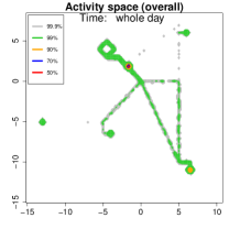
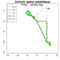
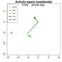
Figure 12 depicts the contour region $Q_{\rho}$ , which encloses the spatial area where the individual spends a proportion $\rho$ of their time. We show contours for $\rho\in\{0.999,0.99,0.90,0.70,0.50\}$ in three scenarios:

1.

All Days (Left Panel): Over 90 days, 90% of the individual’s time (orange contour) is concentrated at home and office, consistent with Patterns 1 and 2 being selected more frequently.
2.

Weekdays (Middle Panel): On weekdays alone, the same 90% region again focuses heavily on home and office, indicating most weekday hours are spent in these two anchor locations.
3.

Weekends (Right Panel): On weekends (Patterns 3 to 5), more than 90% of time is spent at home, reflecting fewer trips away from the house (with occasional visits to the supermarket or beach).

B.3.3 Clustering of trajectories

Clustering of days. A key aspect of our study is to cluster the simulated individual’s weekday days (Patterns 1 and 2) and weekend days (Patterns 3, 4, and 5) based on their GPS trajectories. To do so, we separately analyze the weekday observations and the weekend observations.

For each day, we compute the smoothed conditional density $\widehat{f}_{c}$ (using the bandwidths $h_{X}$ and $h_{T}$ determined earlier) and measure pairwise distances via the integrated squared difference between log-densities:

D_{ij}\;=\;\int\Bigl{[}\log\bigl{(}\widehat{f}_{c,i}(x)+\xi\bigr{)}\;-\;\log\bigl{(}\widehat{f}_{c,j}(x)+\xi\bigr{)}\Bigr{]}^{2}\,dx,

where $\widehat{f}_{c,i}$ is the estimated conditional density for day $i$ , and $\widehat{f}_{c,j}$ for day $j$ . Same as the log-density visualization in Figure 10, here, $\xi$ is set as 0.0001.

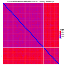
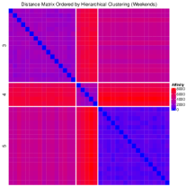
Figure 13 further illustrates the structure of the clusters by showing the re-ordered distance matrices for weekdays (left panel) and weekends (right panel). In both cases, we see a pronounced block structure, indicating clear separations between the different activity patterns measured based on our proposed density estimation method.

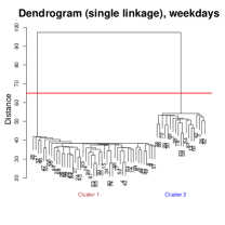
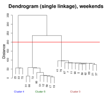
We perform single-linkage hierarchical clustering, producing dendrograms of weekday and weekend data (Figure 14). After comparing with the known activity pattern for each day, we find that hierarchical clustering achieves 100% accurate day-level classifications, perfectly matching the original activity patterns used to generate the data.

Conditional density on clustered days. To further illustrate how the discovered clusters differ in their spatiotemporal patterns, we compare conditional densities at specific times of day.

Figure 15 shows the estimated conditional density at 6:00 PM for each weekday cluster (i.e., Patterns 1 and 2). The densities differ markedly: in Pattern 1, the individual leaves the office and goes directly home, whereas in Pattern 2, they stop at a restaurant (top-right anchor) before returning home.

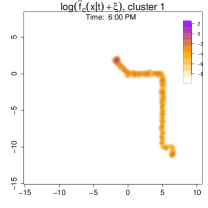
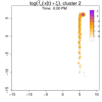
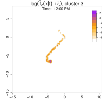
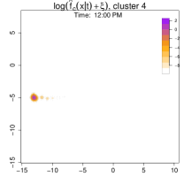
Figure 16 displays the conditional density at 12:00 PM for each weekend cluster. In Pattern 3, the individual is often near the supermarket around noon; in Pattern 4, they might be found at the beach; and in Pattern 5, they remain at home throughout the day.

Centers on each cluster. Given these day-level clusters, we also estimate a cluster-specific center $\widehat{\mu}_{g}(t)$ representing the average location for each cluster at time $t$ . Figure 17 shows the computed centers at six time points (from 6:00 AM to 9:00 PM) for each cluster. The first (top-left) panel shows the combined data (all days), and the remaining panels correspond to each of the five clusters.

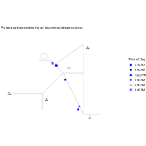
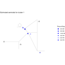
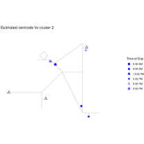
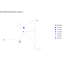
On weekdays, for four of the six time points 6:00 AM, 12:00 PM, 3:00 PM, and 9:00 PM, both clusters have roughly the same center (reflecting time spent at home or in the office). However, at 9:00 AM, the Cluster 1 center is closer to home, whereas the Cluster 2 center is closer to the office, consistent with the expected earlier departure in the weekdays’ morning under Pattern 2 in Table 1. At 6:00 PM, Cluster 1 centers near home, while Cluster 2 centers near the restaurant, mirroring the aforementioned difference in post-work behavior.

Each weekend pattern displays a distinct midday center, aligning with the anchor points for each pattern on weekends: supermarket for Pattern 3, beach for Pattern 4, and home for Pattern 5.

Appendix C Assumptions

Assumption 1 (Property of the kernel function)

The 2-dimensional kernel function $K(x)$ satisfies the following properties:

(a) $K(x)\geq 0$ for any $x\in\mathbb{R}^{2}$ ;

(b) $K(x)$ is symmetric, i.e. for any $x_{1},x_{2}\in\mathbb{R}^{2}$ satisfying $\|x_{1}\|_{2}=\|x_{2}\|_{2}$ , we have $K(x_{1})=K(x_{2})$ ;

(d) $\int x^{T}xK(x)dx<\infty$ .

(e) $K$ have Lipchitz property: there exists constant $L_{K}$ such that, for any $x_{1},x_{2}\in\mathbb{R}^{2}$ , we have

\displaystyle|K(x_{1})-K(x_{2})|\leq L_{K}\|x_{1}-x_{2}\|.

Assumption 1 are standard assumptions on the kernel functions (Wasserman, , 2006). The additional requirement is the Lipchitz condition (e) but it is a very mild condition.

Assumption 2

Any random trajectory $S(t)$ is Lipschitz, i.e., there exists a $\bar{v}<\infty$ such that $\|S(t_{1})-S(t_{2})\|\leq\bar{v}d_{T}(t_{1},t_{2})$ for any $t_{1},t_{2}$ .

The Lipschitz condition in Assumption 2 allows the case where the individual suddenly start moving. It also implies that the velocity of the individual is finite (the Lipschitz constant).

Assumption 3

The density of measurement error $f_{\epsilon}$ is bounded in the sense that $\|f_{\epsilon}(\eta)\|$ , $\|\nabla f_{\epsilon}(\eta)\|$ , and $\|\nabla\nabla f_{\epsilon}(\eta)\|_{2}$ are uniformly bounded by a constant $M_{\epsilon}$ for every $\eta\in\mathbb{R}^{2}$ .

The Assumption 1 is the common assumption for kernel density estimation, and most common kernel functions can satisfy it. When the distribution of measurement error is fixed, then the Assumption 3 is automatically satisfied.

By the convolution theory, Assumptions 3 implies that the GPS density $f_{GPS}$ has bounded second derivative.

Assumption 4

The kernel function $K_{T}$ is a symmetric PDF and $\int t^{2}K(t)dt<\infty$ and is Lipschitz.

Assumption 4 is for the kernel function on the time. It will be used when we analyze the asymptotic properties of the conditional estimator.

Appendix D Proofs

D.1 Proof of Proposition 1

Proof. By definition of $f_{GPS}$ in (1),

\displaystyle f_{GPS}(x)=\lim_{r\rightarrow 0}\frac{P(X^{*}\in B(x,r))}{\pi r^{2}}=\lim_{r\rightarrow 0}\frac{P(S(U)+\epsilon\in B(x,r))}{\pi r^{2}}.

Since $U\sim{\sf Uniform}([0,1])$ , we have

	$\displaystyle\lim_{r\rightarrow 0}\frac{P(S(U)+\epsilon\in B(x,r))}{\pi r^{2}}$	$\displaystyle=\lim_{r\rightarrow 0}\frac{\int P(S(U)+\epsilon\in B(x,r)\|U=t)dt}{\pi r^{2}}$
		$\displaystyle=\lim_{r\rightarrow 0}\frac{\int_{t\in[0,1]}P(S(t)+\epsilon\in B(x,r))dt}{\pi r^{2}}$
		$\displaystyle=\lim_{r\rightarrow 0}\frac{\int_{t\in[0,1]}P(X^{*}_{t}\in B(x,r))dt}{\pi r^{2}}.$

Then, by the dominated convergence theorem,

\displaystyle\lim_{r\rightarrow 0}\frac{\int_{t\in[0,1]}P(X^{*}_{t}\in B(x,r))dt}{\pi r^{2}}=\int_{t\in[0,1]}\lim_{r\rightarrow 0}\frac{P(X^{*}_{t}\in B(x,r))}{\pi r^{2}}dt=\int_{0}^{1}f_{GPS}(x|t)dt.

By definition of $f_{GPS,A}$ in (3),

\displaystyle f_{GPS,A}(x)=\lim_{r\rightarrow 0}\frac{P(X^{*}_{A}\in B(x,r))}{\pi r^{2}}=\lim_{r\rightarrow 0}\frac{P(S(U_{A})+\epsilon\in B(x,r))}{\pi r^{2}}.

Since $U_{A}\sim{\sf Uniform}(A)$ , then by the same reasoning,

\displaystyle\lim_{r\rightarrow 0}\frac{P(S(U_{A})+\epsilon\in B(x,r))}{\pi r^{2}}=\lim_{r\rightarrow 0}\frac{\int_{t\in A}P(S(t)+\epsilon\in B(x,r))\frac{1}{|A|}dt}{\pi r^{2}}=\lim_{r\rightarrow 0}\frac{1}{|A|}\frac{\int_{t\in A}P(X^{*}_{t}\in B(x,r))dt}{\pi r^{2}}.

Similarly, by the dominated convergence theorem, we have

\displaystyle\lim_{r\rightarrow 0}\frac{1}{|A|}\frac{\int_{t\in A}P(X^{*}_{t}\in B(x,r))dt}{\pi r^{2}}=\int_{t\in A}\lim_{r\rightarrow 0}\frac{1}{|A|}\frac{P(X^{*}_{t}\in B(x,r))}{\pi r^{2}}dt=\frac{1}{|A|}\int_{A}f_{GPS}(x|t)dt.

$\Box$

D.2 Proof of Proposition 2

Proof. By definition of $f_{GPS}$ in (1),

\displaystyle f_{GPS}(a)=\lim_{r\rightarrow 0}\frac{P(X^{*}\in B(a,r))}{\pi r^{2}}=\lim_{r\rightarrow 0}\frac{P(S(U)+\epsilon\in B(a,r))}{\pi r^{2}}.

Since $U\sim{\sf Uniform}([0,1])$

		$\displaystyle P(S(U)+\epsilon\in B(a,r))$
	$\displaystyle\geq$	$\displaystyle P(S(U)+\epsilon\in B(a,r),S(U)=a)$
	$\displaystyle=$	$\displaystyle P(S(U)+\epsilon\in B(a,r)\|S(U)=a)P(S(U)=a)$
	$\displaystyle=$	$\displaystyle P(S(U)=a)P(\epsilon\in B(0,r))$
	$\displaystyle\geq$	$\displaystyle\rho_{a}P(\epsilon\in B(0,r)).$

Note that

\displaystyle\lim_{r\rightarrow 0}\frac{P(\epsilon\in B(y,r))}{\pi r^{2}}=\frac{1}{2\pi\sigma^{2}}\exp\left\{-\frac{y^{T}y}{2\sigma^{2}}\right\},

for any $y\in\mathbb{R}^{2}$ . Hence, $\lim_{r\rightarrow 0}\frac{P(\epsilon\in B(0,r))}{\pi r^{2}}=\frac{1}{2\pi\sigma^{2}}$ . Then,

\displaystyle\lim_{r\rightarrow 0}\frac{P(S(U)+\epsilon\in B(a,r))}{\pi r^{2}}\geq\frac{\rho_{a}}{2\pi\sigma^{2}}.

For regular GPS density $f_{GPS}(x)$ , we have

\displaystyle\int_{B(a,r)}f_{GPS}(x)dx=P(S(U)+\epsilon\in B(a,r))\geq P(S(U)=a,S(U)+\epsilon\in B(a,r)).

Moreover, the right-hand-side in the above inequality can further be bound by

		$\displaystyle P(S(U)=a,S(U)+\epsilon\in B(a,r))$
	$\displaystyle=$	$\displaystyle P(S(U)+\epsilon\in B(a,r)\|S(U)=a)P(S(U)=a)$
	$\displaystyle\geq$	$\displaystyle\rho_{a}P(\epsilon\in B(0,r)\|S(U)=a)$
	$\displaystyle=$	$\displaystyle{\rho_{a}}F_{\chi^{2}_{2}}\left(\frac{r^{2}}{\sigma^{2}}\right).$

Note that we use the fact that $\epsilon$ is an isotropic Gaussian with a variance $\sigma^{2}$ , so

P(\epsilon\in B(0,r))=P(\epsilon^{2}\leq r^{2})=P\left(\frac{\epsilon^{2}}{\sigma^{2}}\leq\frac{r^{2}}{\sigma^{2}}\right)=F_{\chi^{2}_{2}}\left(\frac{r^{2}}{\sigma^{2}}\right).

$\Box$

D.3 Proof of Proposition 3

Proof. We can write $\int_{C\oplus r}f_{GPS}(x)dx$ as

		$\displaystyle\int_{C\oplus r}f_{GPS}(x)dx=P(S(U)+\epsilon\in C\oplus r)$
	$\displaystyle\geq$	$\displaystyle P(S(U)\in C,S(U)+\epsilon\in C\oplus r)$
	$\displaystyle\geq$	$\displaystyle P(S(U)\in C,S(U)+\epsilon\in B(S(U),r))$
	$\displaystyle=$	$\displaystyle P(S(U)\in C,\epsilon\in B(0,r))$
	$\displaystyle=$	$\displaystyle P(S(U)\in C)P(\epsilon\in B(0,r))$
	$\displaystyle\geq$	$\displaystyle\rho_{C}F_{\chi^{2}_{2}}\left(\frac{r^{2}}{\sigma^{2}}\right).$

$\Box$

D.4 Proof of Proposition 4

Proof. A straight forward calculation shows that

	$\displaystyle G_{C}\leq\int_{C}f_{GPS}(x)dx$	$\displaystyle=P(S(U)+\epsilon\in C)$
		$\displaystyle=P(S(U)+\epsilon\in C,\epsilon\leq r)+P(S(U)+\epsilon\in C,\epsilon>r)$
		$\displaystyle\leq P(S(U)+\epsilon\in C,\epsilon\leq r)+P(\epsilon>r)$
		$\displaystyle\leq P(S(U)+\epsilon\in C\|\epsilon\leq r)P(\epsilon\leq r)+1-F_{\chi^{2}_{2}}\left(\frac{r^{2}}{\sigma^{2}}\right)$
		$\displaystyle\leq P(S(U)+\epsilon\in C\|\epsilon\leq r)F_{\chi^{2}_{2}}\left(\frac{r^{2}}{\sigma^{2}}\right)+1-F_{\chi^{2}_{2}}\left(\frac{r^{2}}{\sigma^{2}}\right).$

Given $\epsilon\leq r$ , a necessary condition to $S(U)+\epsilon\in C$ is that $S(U)\in C\oplus r$ . Thus,

P(S(U)+\epsilon\in C|\epsilon\leq r)\leq P(S(U)\in C\oplus r).

Putting this into the long inequality shows that

G_{C}\leq P(S(U)\in C\oplus r)F_{\chi^{2}_{2}}\left(\frac{r^{2}}{\sigma^{2}}\right)+1-F_{\chi^{2}_{2}}\left(\frac{r^{2}}{\sigma^{2}}\right),

which is the desired result after rearrangements.

$\Box$

D.5 Proof of Theorem 5

Let $\widehat{f}_{w,i}(x)$ is the estimated density of $i-$ th day observations, i.e.

\displaystyle\widehat{f}_{w,i}(x)=\frac{1}{h^{2}}\sum_{i=1}^{m_{i}}\frac{(t_{i,j+1}-t_{i,j-1})}{2}K\left(\frac{x-X_{i,j}}{h}\right).

Since the latent trajectories across different days are IID, this estimator will be IID quantities in different days if the timestamps $\{t_{i,j}:j=1,\ldots,m_{i}\}$ are the same for every $i$ . Since the time-weighted estimator can be written as the mean of each day, i.e.,

\widehat{f}_{w}(x)=\frac{1}{n}\sum_{i=1}^{n}\widehat{f}_{w,i}(x),

we can investigate the bias of $\widehat{f}_{w}$ by investigating the bias of $\widehat{f}_{w,i}$ versus $f_{GPS}$ . The following lemma will be useful for this purpose.

Lemma 8 (Riemannian integration approximation of GPS density)

Assume assumptions 1 to 3. For any $i\in\{1,...,n\}$ and a trajectory $s\in\mathcal{S}$ , there are constants $C_{\bar{v}},M_{\epsilon}$ such that $C_{\bar{v}}$ depends on the maximal velocity of $s$ and $M_{\epsilon}$ depends on the distribution of $\epsilon$ with

\displaystyle\mathbb{E}\left[\widehat{f}_{w,i}(x)\mid S_{i}=s\right]-\mathbb{E}\left[\frac{1}{h^{2}}K\left(\frac{x-X^{*}}{h}\right)\mid S_{i}=s\right]

\displaystyle\leq C_{\bar{v}}\left(\frac{1}{nh^{3}}\sum_{j=0}^{m_{i}}(t_{i,j+1}-t_{i,j})^{2}\right)

(24)

for every $x\in\mathbb{R}^{2}$ .

Proof.[Proof of Lemma 8] Since $S_{1},...,S_{n}\sim_{i.i.d}P_{S}$ , without loss of generality, we only need to derive (24) under $i=1$ . Then, for $i=1$ , we can decompose (24) to the following two terms:

$\displaystyle\mathbb{E}\left[\widehat{f}_{w,1}(x)\mid S_{1}=s\right]$	$\displaystyle-\mathbb{E}\left[\frac{1}{h^{2}}K\left(\frac{x-X^{*}}{h}\right)\mid S_{1}=s\right]$	(25)
	$\displaystyle=\underbrace{\frac{1}{h^{2}}\sum_{j=1}^{m_{1}}\frac{(t_{1,j+1}-t_{1,j-1})}{2}\int_{\epsilon_{1,j}}K\left(\frac{x-s(t_{1,j})+\epsilon_{1,j}}{h}\right)dF_{\epsilon}(\epsilon_{1,j})}_{(I)}$
	$\displaystyle-\underbrace{\frac{1}{h^{2}}\int_{\nu}\int_{u\in[0,1]}K\left(\frac{x-s(u)+\nu}{h}\right)dudF_{\epsilon}(\nu)}_{(II)}.$

To simplify in (25), we use $I_{h}(t_{1,j};s,x)$ to denote $\int_{\epsilon_{1,j}}K\left(\frac{x-s(t_{1,j})+\epsilon_{1,j}}{h}\right)dF_{\epsilon}$ , i.e. the expection of $K\left(\frac{x-X_{1,j}}{h}\right)$ at time $t_{1,j}$ given latent trajectory $S_{1}=s$ .

Term (I): Then, by $t_{1,j+1}-t_{1,j-1}=(t_{1,j+1}-t_{1,j})+(t_{1,j}-t_{1,j-1})=\int_{t_{1,j}}^{t_{1,j+1}}du+\int_{t_{1,j-1}}^{t_{1,j}}du$ , Term (I) in (25) can be written as

		$\displaystyle\frac{1}{h^{2}}\sum_{j=1}^{m_{1}}\frac{(t_{1,j+1}-t_{1,j-1})}{2}I_{h}(t_{1,j};s,x)$
	$\displaystyle=$	$\displaystyle\frac{(t_{1,1}-t_{1,0})}{2}I_{h}(t_{1,1};s,x)+\frac{(t_{1,m_{1}+1}-t_{1,m})}{2}I_{h}(t_{1,m};s,x)+\frac{1}{h^{2}}\sum_{j=1}^{m_{1}-1}\frac{(t_{1,j+1}-t_{1,j})}{2}I_{h}(t_{1,j};s,x).$

For the weights of first and last observation, note that,

\displaystyle\frac{(t_{1,1}-t_{1,0})}{2}=\frac{(t_{1,m_{1}+1}-t_{1,m_{1}})}{2}=\frac{1-(t_{1,m_{1}}-t_{1,1})}{2}=\frac{1}{2}\left[\int_{0}^{t_{1,1}}1du+\int_{t_{1,m_{1}}}^{1}1du\right].

We have

	$\displaystyle\frac{1}{h^{2}}\sum_{j=1}^{m_{1}}\frac{(t_{1,j+1}-t_{1,j-1})}{2}I_{h}(t_{1,j};s,x)$
$\displaystyle=$	$\displaystyle\frac{1}{h^{2}}\sum_{j=1}^{m_{1}-1}\int_{t_{1,j}}^{t_{1,j+1}}I_{h}(t_{1,j};s,x)du+\frac{1}{2h^{2}}\left[\int_{0}^{t_{1,1}}I_{h}(t_{1,1};s,x)du+\int_{t_{1,m_{1}}}^{1}I_{h}(t_{1,1};s,x)du\right]+$
	$\displaystyle\frac{1}{2h^{2}}\left[\int_{0}^{t_{1,1}}I_{h}(t_{1,m_{1}};s,x)du+\int_{t_{1,m_{1}}}^{1}I_{h}(t_{1,m_{1}};s,x)du\right].$	(26)

Term (II): Note that $I_{h}(u;s,x)=\int_{\epsilon}K\left(\frac{x-s(u)+\nu)}{h}\right)dF_{\epsilon}(\nu)$ , then Term (II) in the (25) can be decomposed to

	$\displaystyle\frac{1}{h^{2}}\int_{\nu}\int_{u\in[0,1]}K\left(\frac{x-s(u)+\nu}{h}\right)dudF_{\epsilon}(\nu)$
$\displaystyle=$	$\displaystyle\frac{1}{h^{2}}\int_{u\in[0,1]}I_{h}(u;s,x)du$
$\displaystyle=$	$\displaystyle\frac{1}{h^{2}}\left[\int_{0}^{t_{1,1}}I_{h}(u;s,x)du+\int_{t_{1,1}}^{t_{1,m_{1}}}I_{h}(u;s,x)du+\int_{t_{1,m_{1}}}^{1}I_{h}(u;s,x)du\right]$
$\displaystyle=$	$\displaystyle\frac{1}{h^{2}}\sum_{j=1}^{m_{1}-1}\int_{t_{1,j}}^{t_{1,j+1}}I_{h}(u;s,x)du+\frac{1}{h^{2}}\left[\int_{0}^{t_{1,1}}I_{h}(u;s,x)du+\int_{t_{1,m_{1}}}^{1}I_{h}(u;s,x)du\right].$	(27)

Namely, we decompose (II) into each interval $[t_{i,j},t_{i,j+1}]$ so that we can easily compare it with term (I).

Combining (26) and (27), (25) can be written as:

	$\displaystyle\mathbb{E}\left[\widehat{f}_{GPS,1}(x)\mid S_{1}=s\right]-\mathbb{E}\left[\frac{1}{h^{2}}K\left(\frac{x-X^{*}}{h}\right)\mid S_{1}=s\right]$
$\displaystyle=$	$\displaystyle\underbrace{\frac{1}{h^{2}}\sum_{j=1}^{m_{1}-1}\left[\int_{t_{1,j}}^{t_{1,j+1}}I_{h}(t_{1,j};s,x)-I_{h}(u;s,x)du+\right]}_{(III)}+$
	$\displaystyle\underbrace{\frac{1}{2h^{2}}\left[\int_{0}^{t_{1,1}}I_{h}(t_{1,1};s,x)-I_{h}(u;s,x)du+\int_{t_{1,m_{1}}}^{1}I_{h}(t_{1,m_{1}};s,x)-I_{h}(u;s,x)du\right]}_{(IV)}+$
	$\displaystyle\underbrace{\frac{1}{2h^{2}}\left[\int_{0}^{t_{1,1}}I_{h}(t_{1,m_{1}};s,x)-I_{h}(u;s,x)du+\int_{t_{1,m_{1}}}^{1}I_{h}(t_{1,1};s,x)-I_{h}(u;s,x)du\right]}_{(V)}$	(28)

In RHS of (28), the term (III) represents the error caused by the approximation using GPS observations. The source of the term (IV) and (V) is due to our design of circular weights for the first and last observation in each day.

Before deriving the convergence rate of term (III), (IV) and (V) in (28), note that, by Assumption 2 (velocity assumption) and Assumption 1 (Lipchitz property of the kernel function $K$ ), for every $j\in\{1,...,m_{1}\},u\in[0,1]$ the term $\left|K\left(\frac{x-s(t_{1,j})+\epsilon_{1,j}}{h}\right)-K\left(\frac{x-s(u)+\epsilon_{1,j}}{h}\right)\right|$ in the further analysis can be bounded in the following way:

\displaystyle\left|K\left(\frac{x-s(t_{1,j})+\epsilon_{1,j}}{h}\right)-K\left(\frac{x-s(u)+\epsilon_{1,j}}{h}\right)\right|\leq L_{K}\left\|\frac{s(t_{1,j})}{h}-\frac{s(u)}{h}\right\|\leq\frac{L_{K}\bar{v}}{h}d_{T}(t_{1,j},u),

(29)

where $d_{T}(t_{1,j},u)=\min\left\{|t_{1,j}-u|,1-|t_{1,j}-u|\right\}$

Term (III): For the convergence rate of the term (III) in (28), we find that

	$\displaystyle\sum_{j=1}^{m_{1}-1}\left[\int_{t_{1,j}}^{t_{1,j+1}}I_{h}(u;s,x)-I_{h}(t_{1,j};s,x)du\right]$	(30)
$\displaystyle=$	$\displaystyle\frac{1}{h^{2}}\sum_{j=1}^{m_{1}}\int_{t_{1,j}}^{t_{1,j+1}}\int_{\epsilon_{1,j}}K\left(\frac{x-s(t_{1,j})+\epsilon_{1,j}}{h}\right)dF_{\epsilon}(\epsilon_{1,j})du-\frac{1}{h^{2}}\sum_{j=1}^{m_{1}}\int_{t_{1,j}}^{t_{1,j+1}}\int_{\epsilon_{1,j}}K\left(\frac{x-s(u)+\epsilon_{1,j}}{h}\right)dF_{\epsilon}(\epsilon_{1,j})du$
$\displaystyle\leq$	$\displaystyle\frac{1}{h^{2}}\sum_{j=1}^{m_{1}}\int_{t_{1,j}}^{t_{1,j+1}}\int_{\epsilon_{1,j}}\left\|K\left(\frac{x-s(t_{1,j})+\epsilon_{1,j}}{h}\right)-K\left(\frac{x-s(u)+\epsilon_{1,j}}{h}\right)\right\|dF_{\epsilon}(\epsilon_{1,j})du$

In (30), for every $j\in\{1,...,m_{i}\}$ and $u\in[t_{1,j-1},t_{1,j}]$ corresponding to each integral of the summation, we have $d_{T}(u,t_{1,j})\leq t_{1,j+1}-t_{1,j}$ Hence, by applying (29), the term (III) in (28) can be bounded by

	$\displaystyle\frac{1}{h^{2}}\frac{1}{T_{1}}\sum_{j=1}^{m_{1}-1}\left[\int_{t_{1,j}}^{t_{1,j+1}}I_{h}(u;s,x)-I_{h}(t_{1,j};s,x)du\right]$
$\displaystyle\leq$	$\displaystyle\frac{1}{h^{3}}\sum_{j=1}^{m_{1}-1}\int_{t_{1,j}}^{t_{1,j+1}}\int L_{K}\bar{v}d_{T}(t_{1,j},u)dF_{\epsilon}(\epsilon_{1,j})du\quad\quad\text{[By \eqref{eq: Riem-velocity0}]}$
$\displaystyle\leq$	$\displaystyle\frac{1}{2h^{3}}\sum_{j=1}^{m_{1}-1}{\left(t_{1,j+1}-t_{1,j}\right)^{2}}L_{K}\bar{v}\quad\quad\text{[By }d_{T}(u,t_{1,j})\leq t_{1,j+1}-t_{1,j}]$
$\displaystyle\leq$	$\displaystyle C_{\bar{v}}\frac{\sum_{j=1}^{m_{1}-1}\left(t_{1,j+1}-t_{1,j}\right)^{2}}{h^{3}},$	(31)

for some constant $C_{\bar{v}}$ .

Term (IV): For term (IV):

	$\displaystyle\frac{1}{2h^{2}}\left[\int_{0}^{t_{1,1}}I_{h}(t_{1,1};s,x)-I_{h}(u;s,x)du+\int_{t_{1,m_{1}}}^{1}I_{h}(t_{1,m_{1}};s,x)-I_{h}(u;s,x)du\right]$
$\displaystyle=$	$\displaystyle\frac{1}{2h^{2}}\int_{0}^{t_{1,1}}\int_{\epsilon_{1,1}}K\left(\frac{x-s(t_{1,1})+\epsilon_{1,1}}{h}\right)-K\left(\frac{x-s(u)+\epsilon_{1,j}}{h}\right)dF_{\epsilon}(\epsilon_{1,1})du+$
	$\displaystyle\frac{1}{2h^{2}}\int_{t_{1,m_{1}}}^{1}\int_{\epsilon_{1,m_{1}}}K\left(\frac{x-s(t_{1,m_{1}})+\epsilon_{1,m_{1}}}{h}\right)-K\left(\frac{x-s(u)+\epsilon_{1,m_{1}}}{h}\right)dF_{\epsilon}(\epsilon_{1,m_{1}})du$	(32)

Since two parts in (32) have same form, we only need to focus on the first term for RHS of (32). Recall $t_{1,0}=t_{1,m}-1$ , then, for $u\in[0,t_{1,1}]$ , $d_{T}(t_{1,1},u)\leq t_{1,1}\leq t_{1,1}-t_{1,0}$ . Thus,

	$\displaystyle\frac{1}{2h^{2}}\int_{0}^{t_{1,1}}\int_{\epsilon_{1,1}}K\left(\frac{x-s(t_{1,1})+\epsilon_{1,1}}{h}\right)-K\left(\frac{x-s(u)+\epsilon_{1,1}}{h}\right)dF_{\epsilon}(\epsilon_{1,1})du$
$\displaystyle\leq$	$\displaystyle\frac{1}{2h^{2}}\int_{0}^{t_{1,1}}\int_{\epsilon_{1,1}}\left\|K\left(\frac{x-s(t_{1,1})+\epsilon_{1,1}}{h}\right)-K\left(\frac{x-s(u)+\epsilon_{1,1}}{h}\right)\right\|dF_{\epsilon}(\epsilon_{1,1})du$
$\displaystyle\leq$	$\displaystyle\frac{1}{2h^{3}}\int_{0}^{t_{1,1}}\int L_{K}\bar{v}d_{T}(t_{1,1},u)dF_{\epsilon}(\epsilon_{1,1})du\quad\quad\text{[By \eqref{eq: Riem-velocity0}]}$
$\displaystyle\leq$	$\displaystyle C_{\bar{v}}\frac{\left(t_{1,1}-t_{1,0}\right)^{2}}{2h^{3}}.$	(33)

Similarly, for the second term of RHS of (32), we have

\displaystyle\frac{1}{2h^{2}}\int_{t_{1,m_{1}}}^{1}\int_{\epsilon_{1,m_{1}}}K\left(\frac{x-s(t_{1,m_{1}})+\epsilon_{1,m_{1}}}{h}\right)-K\left(\frac{x-s(u)+\epsilon_{1,m_{1}}}{h}\right)dF_{\epsilon}(\epsilon_{1,m_{1}})du\leq C_{\bar{v}}\frac{\left(t_{1,m_{1}+1}-t_{1,m_{1}}\right)^{2}}{2h^{3}}.

(34)

Term (V): For term (V):

	$\displaystyle\frac{1}{2h^{2}}\left[\int_{0}^{t_{1,1}}I_{h}(t_{1,m_{1}};s,x)-I_{h}(u;s,x)du+\int_{t_{1,m_{1}}}^{1}I_{h}(t_{1,1};s,x)-I_{h}(u;s,x)du\right]$
$\displaystyle=$	$\displaystyle\frac{1}{2h^{2}}\int_{0}^{t_{1,1}}\int_{\epsilon_{1,m_{1}}}K\left(\frac{x-s(t_{1,m_{1}})+\epsilon_{1,m_{1}}}{h}\right)-K\left(\frac{x-s(u)+\epsilon_{1,m_{1}}}{h}\right)dF_{\epsilon}(\epsilon_{1,m_{1}})du+$
	$\displaystyle\frac{1}{2h^{2}}\int_{t_{1,m_{1}}}^{1}\int_{\epsilon_{1,1}}K\left(\frac{x-s(t_{1,1})+\epsilon_{1,1}}{h}\right)-K\left(\frac{x-s(u)+\epsilon_{1,1}}{h}\right)dF_{\epsilon}(\epsilon_{1,1})du$	(35)

Similar as the procedure of deriving convergence rate of term (IV), the two parts in RHS of (35) have same form, we only need to focus on the first term for RHS of (35), for $u\in[0,t_{1,1}]$ , $d_{T}(t_{1,m_{1}},u)\leq 1-(t_{1,m_{1}}-t_{1,1})=t_{1,m_{1}+1}-t_{1,m_{1}}$ . Thus,

	$\displaystyle\frac{1}{2h^{2}}\int_{0}^{t_{1,1}}\int_{\epsilon_{1,1}}K\left(\frac{x-s(t_{1,m_{1}})+\epsilon_{1,m_{1}}}{h}\right)-K\left(\frac{x-s(u)+\epsilon_{1,m_{1}}}{h}\right)dF_{\epsilon}(\epsilon_{1,m_{1}})du$
$\displaystyle\leq$	$\displaystyle\frac{1}{2h^{2}}\int_{0}^{t_{1,1}}\int_{\epsilon_{1,1}}\left\|K\left(\frac{x-s(t_{1,m_{1}})+\epsilon_{1,m_{1}}}{h}\right)-K\left(\frac{x-s(u)+\epsilon_{1,m_{1}}}{h}\right)\right\|dF_{\epsilon}(\epsilon_{1,m_{1}})du$
$\displaystyle\leq$	$\displaystyle\frac{1}{2h^{3}}\int_{0}^{t_{1,1}}\int L_{K}\bar{v}d_{T}(t_{1,m_{1}},u)dF_{\epsilon}(\epsilon_{1,1})du\quad\quad\text{[By \eqref{eq: Riem-velocity0}]}$
$\displaystyle\leq$	$\displaystyle C_{\bar{v}}\frac{\left(t_{1,m_{1}+1}-t_{1,m_{1}}\right)^{2}}{2h^{3}}.$	(36)

Similarly,

\displaystyle\frac{1}{2h^{2}}\int_{t_{1,m_{1}}}^{1}\int_{\epsilon_{1,1}}K\left(\frac{x-s(t_{1,1})+\epsilon_{1,1}}{h}\right)-K\left(\frac{x-s(u)+\epsilon_{1,1}}{h}\right)dF_{\epsilon}(\epsilon_{1,1})du\leq C_{\bar{v}}\frac{\left(t_{1,1}-t_{1,0}\right)^{2}}{2h^{3}}

(37)

Hence, combining (31), (33), (34) and (36), (37), for every $x\in\mathcal{W}$ , there is constant $C_{\bar{v}}$ such that

\displaystyle\mathbb{E}\left[\widehat{f}_{w,i}(x)\mid S=s\right]-\mathbb{E}\left[\frac{1}{h^{2}}K\left(\frac{x-X^{*}}{h}\right)\mid S=s\right]\leq C_{\bar{v}}\left(\frac{1}{nh^{3}}\sum_{i=1}^{n}\sum_{j=0}^{m_{k}}(t_{i,j+1}-t_{i,j})^{2}\right)

$\Box$

Proof. For any $x$ , $f_{GPS}(x)-\widehat{f}_{w}(x)$ can be decomposed to the following three terms:

\displaystyle f_{GPS}(x)-\widehat{f}_{w}(x)=

\displaystyle\underbrace{f_{GPS}(x)-\mathbb{E}\left[\frac{1}{h^{2}}K\left(\frac{x-X^{*}}{h}\right)\right]}_{(I)}+\underbrace{\mathbb{E}\left[\frac{1}{h^{2}}K\left(\frac{x-X^{*}}{h}\right)\right]-\mathbb{E}[\widehat{f}_{w}(x)]}_{(II)}+\underbrace{\mathbb{E}[\widehat{f}_{w}(x)]-\widehat{f}_{w}(x)}_{(III)}.

Term (I): $f_{GPS}(x)-\mathbb{E}\left[\frac{1}{h^{2}}K\left(\frac{x-X^{*}}{h}\right)\right]$ ; For any $x\in\mathbb{R}^{2}$ , we have

		$\displaystyle f_{GPS}(x)-\mathbb{E}\left[\frac{1}{h^{2}}K\left(\frac{x-X^{*}}{h}\right)\right]$
	$\displaystyle=$	$\displaystyle\frac{1}{h^{2}}\int_{y\in\mathbb{R}^{2}}K\left(\frac{x-y}{h}\right)f_{GPS}(y)dy-f_{GPS}(x)$
	$\displaystyle=$	$\displaystyle\int_{z\in\mathbb{R}^{2}}K\left(z\right)f_{GPS}(x-hz)dz-f_{GPS}(x)$

By Assumption 3, $f_{GPS}$ is twice differentiable,

	$\displaystyle\int_{z\in\mathbb{R}^{2}}K\left(z\right)f_{GPS}(x-hz)dz-f_{GPS}(x)=$	$\displaystyle\int_{y\in\mathbb{R}^{2}}K\left(z\right)f_{GPS}(x)+hz^{T}\nabla f_{GPS}(x)$
		$\displaystyle+h^{2}z^{T}\nabla\nabla f_{GPS}(x)zdz-f_{GPS}(x)+o(h^{2}).$

By Assumption 1 and Assumption 3, $\int_{z\in\mathbb{R}^{2}}K(z)dz=1$ , $\int_{z\in\mathbb{R}^{2}}zK(z)dz=0$ , $\nabla\nabla f_{GPS}$ is bounded. Hence,

\displaystyle\int_{z\in\mathbb{R}^{2}}K\left(z\right)f_{GPS}(x-hz)dz-f_{GPS}(x)=O(h^{2}).

(38)

Term (II): $\mathbb{E}\left[\frac{1}{h^{2}}K\left(\frac{x-X^{*}}{h}\right)\right]-\mathbb{E}[\widehat{f}_{w}(x)]$ . Recall that $\widehat{f}_{w,i}(x)$ to is the estimated density contributed by the observations in $i-$ th day, i.e.

\displaystyle\widehat{f}_{w,i}(x)=\frac{1}{h^{2}}\sum_{j=1}^{m_{i}}\frac{(t_{i,j+1}-t_{i,j-1})}{2}K\left(\frac{x-X_{i,j}}{h}\right).

Then, we can decompose the expectation of the density estimator:

		$\displaystyle\mathbb{E}\left[\widehat{f}_{w}(x)\right]$
	$\displaystyle=$	$\displaystyle\frac{1}{2nh^{2}}\sum_{i=1}^{n}\mathbb{E}\left[\sum_{j=1}^{m_{i}}{(t_{i,j+1}-t_{i,j-1})}K\left(\frac{x-X_{i,j}}{h}\right)\right]$
	$\displaystyle=$	$\displaystyle\frac{1}{2nh^{2}}\sum_{i=1}^{n}\mathbb{E}\left\{\mathbb{E}\left[\sum_{j=1}^{m_{i}}{(t_{i,j+1}-t_{i,j-1})}K\left(\frac{x-X_{i,j}}{h}\right)\mid S_{i}\right]\right\}$
	$\displaystyle=$	$\displaystyle\frac{1}{2nh^{2}}\sum_{i=1}^{n}\sum_{j=1}^{m_{i}}{(t_{i,j+1}-t_{i,j-1})}\int_{s\in\mathcal{S}}\int_{\epsilon_{i,j}}K\left(\frac{x-s(t_{i,j})+\epsilon_{i,j}}{h}\right)dF_{S}(s)dF_{\epsilon}(\epsilon_{i,j})$
	$\displaystyle\triangleq$	$\displaystyle\frac{1}{n}\sum_{i=1}^{n}\int_{s\in\mathcal{S}}\mathbb{E}\left[\widehat{f}_{w,i}(x)\mid S=s\right]dF_{S}(s),$

Note that

\mathbb{E}\left[\frac{1}{h^{2}}K\left(\frac{x-X^{*}}{h}\right)\right]=\int_{s\in\mathcal{S}}\mathbb{E}\left[\frac{1}{h^{2}}K\left(\frac{x-X^{*}}{h}\right)|S=s\right]dF_{S}(s).

Hence, term (II) can be written as

\displaystyle\mathbb{E}[\widehat{f}_{w}(x)]-\mathbb{E}\left[\frac{1}{h^{2}}K\left(\frac{x-X^{*}}{h}\right)\right]=\frac{1}{n}\sum_{i=1}^{n}\int_{s\in\mathcal{S}}\mathbb{E}\left[\widehat{f}_{w,i}(x)\mid S=s\right]-\mathbb{E}\left[\frac{1}{h^{2}}K\left(\frac{x-X^{*}}{h}\right)|S=s\right]dF_{S}(s).

Then, by Lemma 8, for any $i\in\{1,...,n\}$ and $s\in\mathcal{S}$ , there is uniform constant $C_{\bar{v}}$ such that

\displaystyle\mathbb{E}\left[\widehat{f}_{w,i}(x)\mid S=s\right]-\mathbb{E}\left[\frac{1}{h^{2}}K\left(\frac{x-X^{*}}{h}\right)\mid S=s\right]\leq

\displaystyle C_{\bar{v}}\left(\frac{1}{nh^{3}}\sum_{i=1}^{n}\sum_{j=0}^{m_{i}}(t_{i,j+1}-t_{i,j})^{2}\right)

for every $x\in\mathcal{W}$ . Hence,

\displaystyle\mathbb{E}\left[\widehat{f}_{w}(x)\right]-\mathbb{E}\left[\frac{1}{h^{2}}K\left(\frac{x-X^{*}}{h}\right)\right]=O\left(\frac{1}{nh^{3}}\sum_{i=1}^{n}\sum_{j=0}^{m}(t_{i,j+1}-t_{i,j})^{2}\right).

Term (III). Note that the term (III) is the variance of $\widehat{f}_{w}(x)$ :

\displaystyle\text{Var}[\widehat{f}_{w}(x)]=\text{Var}\left[\frac{1}{nh^{2}}\sum_{i=1}^{n}\sum_{j=1}^{m_{i}}W_{i,j}K\left(\frac{x-S_{i}(t_{i,j})+\epsilon_{i,j}}{h}\right)\right]=\frac{1}{n^{2}h^{4}}\sum_{i=1}^{n}\text{Var}\left[\sum_{j=1}^{m_{i}}W_{i,j}K\left(\frac{x-S_{i}(t_{i,j})+\epsilon_{i,j}}{h}\right)\right].

by the independence among $\{S_{1},...,S_{n}\}$ . To simplify, we only need to consider $i=1$ . Then we calculate

		$\displaystyle\text{Var}\left[\sum_{j=1}^{m_{1}}W_{i,j}K\left(\frac{x-S(t_{1,j})+\epsilon_{1,j}}{h}\right)\right]$		(39)
	$\displaystyle=$	$\displaystyle\mathbb{E}\left\{\text{Var}\left[\sum_{j=1}^{m_{1}}W_{i,j}K\left(\frac{x-S(t_{1,j})+\epsilon_{1,j}}{h}\right)\|S_{1}\right]\right\}+\text{Var}\left\{\mathbb{E}\left[\sum_{j=1}^{m_{1}}W_{i,j}K\left(\frac{x-S(t_{1,j})+\epsilon_{1,j}}{h}\right)\|S_{1}\right]\right\}.$		(39)

For the first term of the RHS of (39), note that $\epsilon_{1,1},\ldots,\epsilon_{1,m_{1}}$ are IID,

		$\displaystyle\mathbb{E}\left\{\text{Var}\left[\sum_{j=1}^{m_{1}}W_{i,j}K\left(\frac{x-S(t_{1,j}))+\epsilon_{1,j}}{h}\right)\|S_{1}\right]\right\}$
	$\displaystyle=$	$\displaystyle\mathbb{E}\left\{\sum_{i=1}^{m_{1}}{W_{i,j}^{2}}\text{Var}\left[K\left(\frac{x-S(t_{1,j})+\epsilon_{1,j}}{h}\right)\|S_{1}\right]\right\}$
	$\displaystyle\leq$	$\displaystyle\mathbb{E}\left\{\sum_{j=1}^{m_{1}}{W_{i,j}^{2}}\mathbb{E}\left[K\left(\frac{x-S(t_{1,j})+\epsilon_{1,j}}{h}\right)^{2}\|S_{1}\right]\right\}.$

Note that, for any $s\in\mathcal{S}$ , $\mathbb{E}\left[K\left(\frac{x-S(t_{1,j})+\epsilon_{1,j}}{h}\right)^{2}|S=s\right]$ only depends on the measurement error that is independent at each timestamp. Then,

		$\displaystyle\mathbb{E}\left\{\sum_{j=1}^{m_{1}}{W_{i,j}^{2}}\mathbb{E}\left[K\left(\frac{x-S(t_{1,j})+\epsilon_{i,j}}{h}\right)^{2}\|S\right]\right\}$
	$\displaystyle=$	$\displaystyle\mathbb{E}\left\{\sum_{j=1}^{m_{1}}{W_{i,j}^{2}}\int_{\epsilon_{1,j}}K\left(\frac{x-S(t_{1,j})+\epsilon_{1,j}}{h}\right)^{2}f_{\epsilon}(\epsilon_{1,j})d\epsilon_{1,j}\right\}$
	$\displaystyle=$	$\displaystyle\int_{s}\sum_{j=1}^{m_{1}}{W_{i,j}^{2}}\int_{\epsilon_{1,j}}K\left(\frac{x-s(t_{1,j})+\epsilon_{1,j}}{h}\right)^{2}f_{\epsilon}(\epsilon_{1,j})d\epsilon_{1,j}dF_{S}(s)$
	$\displaystyle=$	$\displaystyle h^{2}\sum_{j=1}^{m_{1}}{W_{i,j}^{2}}\int_{s}\int_{u_{1,j}}K\left(u_{1,j}\right)^{2}f_{\epsilon}(u_{1,j}h-x+s(t_{1,j}))du_{1,j}dF_{S}(s).$

By Assumption 1 and 3, $f_{\epsilon}$ and $\int_{x\in\mathbb{R}^{2}}K(x)^{2}dx$ is bounded, we have

\displaystyle h^{2}\sum_{j=1}^{m_{1}}{W_{i,j}^{2}}\int_{s}\int_{\epsilon_{1,j}}K\left(u_{1,j}\right)^{2}f_{\epsilon}(u_{1,j}h-x+s(t_{1,j}))du_{1,j}dF_{S}(s)=O\left({h^{2}}\sum_{j=1}^{m_{1}}W_{i,j}^{2}\right).

(40)

For the second term in RHS of (39), by

		$\displaystyle\text{Var}\left\{\mathbb{E}\left[\sum_{j=1}^{m_{1}}W_{i,j}K\left(\frac{x-S(t_{1,j})+\epsilon_{i,j}}{h}\right)\|S\right]\right\}$		(41)
	$\displaystyle\leq$	$\displaystyle\mathbb{E}\left\{\left\{\mathbb{E}\left[\sum_{j=1}^{m_{1}}W_{i,j}K\left(\frac{x-S(t_{1,j})+\epsilon_{i,j}}{h}\right)\|S\right]\right\}^{2}\right\},$		(41)

we consider $\mathbb{E}\left[\sum_{j=1}^{m_{1}}W_{i,j}K\left(\frac{x-S(t_{1,j})+\epsilon_{i,j}}{h}\right)|S\right]$ in (41) first. For any $s\in\mathcal{S}$ :

		$\displaystyle\mathbb{E}\left[\sum_{j=1}^{m_{1}}W_{i,j}K\left(\frac{x-S(t_{1,j})+\epsilon_{i,j}}{h}\right)\|S=s\right]$
	$\displaystyle=$	$\displaystyle\sum_{j=1}^{m_{1}}W_{i,j}\int_{\epsilon_{1,j}}K\left(\frac{x-s(t_{1,j})+\epsilon_{1,j}}{h}\right)f_{\epsilon}(\epsilon_{1,j})d\epsilon_{1,j}$
	$\displaystyle=$	$\displaystyle h^{2}\sum_{j=1}^{m_{1}}W_{i,j}\int_{\epsilon_{1,j}}K\left(u_{1,j}\right)f_{\epsilon}(u_{1,j}h-x+s(t_{1,j}))du_{1,j}.$

For any $s\in\mathcal{S}$ , $\int_{\epsilon_{1,j}}K\left(u_{1,j}\right)f_{\epsilon}(u_{1,j}h-x+s(t_{1,j}))du_{1,j}$ is upped-bounded by $\max_{y}f_{\epsilon}(y)$ , then the RHS of (41) can be upper-bounded by

		$\displaystyle\mathbb{E}\left\{\left\{\mathbb{E}\left[\sum_{j=1}^{m_{1}}W_{i,j}K\left(\frac{x-S(t_{1,j})+\epsilon_{i,j}}{h}\right)\|S\right]\right\}^{2}\right\}$
	$\displaystyle=$	$\displaystyle\mathbb{E}\left[\left\{h^{2}\sum_{j=1}^{m_{1}}W_{i,j}\int_{\epsilon_{1,j}}K\left(u_{1,j}\right)f_{\epsilon}(u_{1,j}h-x+S(t_{1,j}))du_{1,j}\right]^{2}\right\}$
	$\displaystyle\leq$	$\displaystyle h^{4}\mathbb{E}\left\{\left[\sum_{j=1}^{m_{1}}W_{i,j}\max_{y}f_{\epsilon}(y)\right]^{2}\right\}\leq{h^{4}}\max_{y}f_{\epsilon}(y)^{2}.$

By Assumption 3, $f_{\epsilon}$ is uniformly bounded by some constant. Hence,

\displaystyle\text{Var}\left\{\mathbb{E}\left[\sum_{j=1}^{m_{1}}W_{i,j}K\left(\frac{x-S(t_{1,j})+\epsilon_{i,j}}{h}\right)|S\right]\right\}=O(h^{4}).

(42)

By (40) and (42), we have

\displaystyle\text{Var}[\widehat{f}_{w}(x)]=

\displaystyle\frac{1}{4n^{2}h^{4}}\sum_{i=1}^{n}\text{Var}\left[\sum_{j=1}^{m_{i}}W_{i,j}K\left(\frac{x-S_{i}(t_{i,j})+\epsilon_{i,j}}{h}\right)\right]=O\left(\frac{1}{n^{2}h^{2}}\sum_{i=1}^{n}\sum_{j=1}^{m_{i}}W_{i,j}^{2}\right)+O\left(\frac{1}{n}\right).

Hence, the convergence rate of Term (III) is

\displaystyle\mathbb{E}[\widehat{f}_{w}(x)]-\widehat{f}_{w}(x)=

\displaystyle O_{p}\left(\frac{1}{nh}\sqrt{\sum_{i=1}^{n}\sum_{j=1}^{m_{i}}W_{i,j}^{2}}\right)+O_{p}\left(n^{-\frac{1}{2}}\right)

Combining the convergence rate of 3 terms derived above, we have

\displaystyle\widehat{f}_{w}(x)-f_{w}(x)=

\displaystyle O(h^{2})+O\left(\frac{1}{nh^{3}}\sum_{i=1}^{n}\sum_{j=0}^{m}(t_{i,j+1}-t_{i,j})^{2}\right)+O_{p}\left(\frac{1}{nh}\sqrt{\sum_{i=1}^{n}\sum_{j=1}^{m_{i}}W_{i,j}^{2}}\right)+O_{p}\left(n^{-\frac{1}{2}}\right).

$\Box$

D.6 Proof of Proposition 6

Proof. From equation (11), we have

	$\displaystyle\frac{(S)}{(B)}=o(1)$	$\displaystyle\Longleftrightarrow\frac{m^{2}h^{6}}{nmh^{2}}=o(1)$
		$\displaystyle\Longleftrightarrow\frac{mh^{4}}{n}=o(1)$
		$\displaystyle\Longleftrightarrow mh^{4}=o(n).$

Since the temporal resolution bias (B) is the dominating term, we should choose $h$ to optimize with respect to this, which leads to $h\asymp m^{-1/5}$ when $mh^{4}=o(n)$ . This leads to the inequality $m^{1/5}=o(n)$ when we put $h$ into the inequality $mh^{4}=o(n)$ .

On the other hand, (S) dominates (B) when $n=o(mh^{4})$ and in this case, the optimal smoothing bandwidth is $h\asymp(nm)^{-1/3}$ . By putting this into $n=o(mh^{4})$ , we obtain the inequality $n=o(m^{1/5})$ .

The convergence rates are obtained by simply plug-in these optimal smoothing bandwidth.

Note that at the critical point $n\asymp m^{1/5}$ , we have $m^{1/5}\asymp(nm)^{1/3}$ , so the two choices coincide.

$\Box$

D.7 Proof of Theorem 7

We use $\widehat{f}_{i}(x|t)$ to denote the $i-$ th day’s contribution to $\widehat{f}(x|t)$ , i.e.

\displaystyle\widehat{f}_{i}(x|t)=\frac{1}{h_{X}^{2}}\frac{\sum_{j=1}^{m_{i}}K\left(\frac{d_{T}(t_{i,j},t)}{h_{T}}\right)K\left(\frac{X_{i,j}-x}{h_{X}}\right)}{\sum_{j^{\prime}=1}^{m_{i}}K\left(\frac{d_{T}(t_{i,j^{\prime}},t)}{h_{T}}\right)}.

Recall that $X_{i,j}=S_{i}(t_{i,j})+\epsilon_{i,j}$ , then, for any $s\in\mathcal{S}$ , we define $\widehat{f}_{i}(x|t;s)$ in the following way:

\displaystyle\widehat{f}_{i}(x|t;s)=\frac{1}{h_{X}^{2}}\frac{\sum_{j=1}^{m_{i}}K\left(\frac{d_{T}(t_{i,j},t)}{h_{T}}\right)K\left(\frac{s(t_{i,j})+\epsilon_{i,j}-x}{h_{X}}\right)}{\sum_{j^{\prime}=1}^{m_{i}}K\left(\frac{d_{T}(t_{i,j^{\prime}},t)}{h_{T}}\right)}.

For any $s\in\mathcal{S}$ , we define $f_{GPS}(x|t;s)$ as

\displaystyle f_{GPS}(x|t;s)

\displaystyle=\lim_{r\rightarrow 0}\frac{P(s(t)+\epsilon\in B(x,r))}{\pi r^{2}}=f_{\epsilon}(x-s(t))

(43)

With the above definitions, $\widehat{f}_{i}(x|t)$ and $f_{GPS}(x|t)$ can be written as

\displaystyle\widehat{f}_{i}(x|t)=\int_{s\in\mathcal{S}}\widehat{f}_{i}(x|t;s)dF_{S}(s),\quad f_{GPS}(x|t)=\int_{s\in\mathcal{S}}f_{GPS}(x|t;s)dF_{S}(s).

(44)

Our analysis begins with a lemma controlling the error for a given trajectory $s$ .

Lemma 9

Under Assumption 2 to Assumption 4, for any $i\in\{1,...,n\}$ and $s\in\mathcal{S}$ , we have

\displaystyle\mathbb{E}\left(\widehat{f}_{i}(x|t;s)\right)-f_{GPS}(x|t;s)=O(h_{X}^{2})+O\left(\sum_{j=1}^{m_{i}}\frac{K\left(d_{T}(\frac{t_{i,j},t)}{h_{T}}\right)}{\sum_{j^{\prime}=1}^{m_{i}}K\left(\frac{d_{T}(t_{i,j^{\prime}},t)}{h_{T}}\right)}f_{\epsilon}(x-s(t_{i,j}))-f_{\epsilon}(x-s(t))\right),

(45)

and

\displaystyle\text{Var}\left(\widehat{f}_{i}(x|t;s)\right)=\frac{M_{\epsilon}}{h_{X}^{2}}\sum_{j=1}^{m_{i}}\left[\frac{K\left(\frac{d_{T}(t_{i,j},t)}{h_{T}}\right)}{\sum_{j^{\prime}=1}^{m_{i}}K\left(\frac{d_{T}(t_{i,j^{\prime}},t)}{h_{T}}\right)}\right]^{2}\int_{x\in\mathbb{R}^{2}}K_{1}^{2}(x)dx,

(46)

for any $t\in[0,1]$ , and $x\in\mathcal{W}$ as $h_{X}\rightarrow 0,m_{i}\rightarrow\infty$ for any $i\in\{1,...,n\}$ .

Proof. By the independence among $S_{1},...,S_{n}$ , WLOG, we can just let $i=1$ .

Bias: We first derive the bias of $\widehat{f}_{GPS,1}(x|t)$ , for any $s\in\mathcal{S}$ , by variable changing $y_{1,j}=\frac{s(t_{1,j})+\epsilon_{1,j}-x}{h_{X}},j=1,...,m_{1}$ , and (43), we have

		$\displaystyle\mathbb{E}\left(\widehat{f}_{1}(x\|t;s)\right)-f_{GPS}(x\|t;s)$
	$\displaystyle=$	$\displaystyle\mathbb{E}\left[\frac{1}{h_{X}^{2}}\frac{\sum_{j=1}^{m_{1}}K\left(\frac{d_{T}(t_{1,j},t)}{h_{T}}\right)K\left(\frac{s(t_{1,j})+\epsilon_{1,j}-x}{h_{X}}\right)}{\sum_{j^{\prime}=1}^{m_{1}}K\left(\frac{d_{T}(t_{1,j^{\prime}},t)}{h_{T}}\right)}\right]-f_{\epsilon}(x-s(t))$
	$\displaystyle=$	$\displaystyle\frac{1}{h_{X}^{2}}\sum_{j=1}^{m_{1}}\frac{K\left(\frac{d_{T}(t_{1,j},t)}{h_{T}}\right)}{\sum_{j^{\prime}=1}^{m_{1}}K\left(\frac{d_{T}(t_{1,j},t)}{h_{T}}\right)}\int_{\epsilon_{1,j}\in\mathbb{R}^{2}}K\left(\frac{s(t_{1,j})+\epsilon_{1,j}-x}{h_{X}}\right)f_{\epsilon}(\epsilon_{1,j})d\epsilon_{1,j}-f_{\epsilon}(x-s(t))$
	$\displaystyle=$	$\displaystyle\sum_{j=1}^{m_{1}}\frac{K\left(\frac{d_{T}(t_{1,j},t)}{h_{T}}\right)}{\sum_{j=1}^{m_{1}}K\left(\frac{d_{T}(t_{1,j},t)}{h_{T}}\right)}\int_{y_{1,j}\in\mathbb{R}^{2}}K_{1}\left(y_{1,j}\right)f_{\epsilon}(h_{X}y_{1,j}+x-s(t_{1,j}))dy_{1,j}-f_{\epsilon}(x-s(t)).$

Then, by Assumption 3, we apply Taylor expansion on $f_{\epsilon}(h_{X}y_{1,j}+x-s(t_{1,j}))$ :

		$\displaystyle\sum_{j=1}^{m_{1}}\frac{K_{T}\left(\frac{d_{T}(t_{1,j},t)}{h_{T}}\right)}{\sum_{j=1}^{m_{1}}K_{T}\left(\frac{d_{T}(t_{1,j},t)}{h_{T}}\right)}\int_{y_{1,j}\in\mathbb{R}^{2}}K_{1}\left(y_{1,j}\right)f_{\epsilon}(h_{X}y_{1,j}+x-s(t_{1,j}))dy_{1,j}-f_{\epsilon}(x-s(t))$
	$\displaystyle=$	$\displaystyle\sum_{j=1}^{m_{1}}\frac{K\left(\frac{d_{T}(t_{1,j},t)}{h_{T}}\right)}{\sum_{j^{\prime}=1}^{m_{1}}K\left(\frac{d_{T}(t_{1,j^{\prime}},t)}{h_{T}}\right)}\int_{y_{1,j}\in\mathbb{R}^{2}}K_{1}\left(y_{1,j}\right)[f_{\epsilon}(x-s(t_{1,j}))+h_{X}\nabla f_{\epsilon}(x-s(t_{1,j}))^{T}y_{1,j}+$
		$\displaystyle h_{X}^{2}y_{1,j}^{T}\nabla\nabla f_{\epsilon}(x-s(t_{1,j}))y_{1,j}-f_{\epsilon}(x-s(t))]dy_{1,j}+o(h_{X}^{2}).$

By Assumption 4, $\int_{y\in\mathbb{R}^{2}}K(y)ydy=0$ , then

		$\displaystyle\sum_{j=1}^{m_{1}}\frac{K\left(\frac{d_{T}(t_{1,j},t)}{h_{T}}\right)}{\sum_{j^{\prime}=1}^{m_{1}}K\left(\frac{d_{T}((t_{1,j^{\prime}},t)}{h_{T}}\right)}\int_{y_{1,j}\in\mathbb{R}^{2}}K\left(y_{1,j}\right)[f_{\epsilon}(x-s(t_{1,j}))+h_{X}\nabla f_{\epsilon}(x-s(t_{1,j}))^{T}y_{1,j}$
		$\displaystyle+h_{X}^{2}y_{1,j}^{T}\nabla\nabla f_{\epsilon}(x-s(t_{1,j}))y_{1,j}-f_{\epsilon}(x-s(t))]dy_{1,j}+o(h_{X}^{2})$
	$\displaystyle=$	$\displaystyle\sum_{j=1}^{m_{1}}\frac{K\left(\frac{d_{T}(t_{1,j},t)}{h_{T}}\right)}{\sum_{j^{\prime}=1}^{m_{1}}K\left(\frac{d_{T}(t_{1,j},t)}{h_{T}}\right)}\int_{y_{1,j}\in\mathbb{R}^{2}}K\left(y_{1,j}\right)[f_{\epsilon}(x-s(t_{1,j}))-f_{\epsilon}(x-s(t))+$
		$\displaystyle h_{X}^{2}y_{1,j}^{T}\nabla\nabla f_{\epsilon}(x-s(t_{1,j}))y_{1,j}]dy_{1,j}+o(h_{X}^{2})$
	$\displaystyle\leq$	$\displaystyle M_{\epsilon}h_{X}^{2}+\sum_{j=1}^{m_{1}}\frac{K\left(\frac{d_{T}(t_{1,j},t)}{h_{T}}\right)}{\sum_{j^{\prime}=1}^{m_{1}}K\left(\frac{d_{T}(t_{1,j^{\prime}},t)}{h_{T}}\right)}f_{\epsilon}(x-s(t_{1,j}))-f_{\epsilon}(x-s(t)).$

Hence,

\displaystyle\mathbb{E}\widehat{f}_{i}(x|t;s)-f_{GPS}(x|t;s)=O(h_{X}^{2})+O\left(\sum_{j=1}^{m_{i}}\frac{K\left(\frac{d_{T}(t_{i,j},t)}{h_{T}}\right)}{\sum_{j^{\prime}=1}^{m_{i}}K\left(\frac{d_{T}(t_{i,j^{\prime}},t)}{h_{T}}\right)}f_{\epsilon}(x-s(t_{i,j}))-f_{\epsilon}(x-s(t))\right).

for any $i\in\{1,...,n\}$

Step 2 (Variance): As for the variance, for any $s\in\mathcal{S}$ ,

$\displaystyle\text{Var}\left(\widehat{f}_{1}(x\|t;s)\right)=$	$\displaystyle\text{Var}\left(\frac{1}{h_{X}^{2}}\frac{\sum_{j=1}^{m_{1}}K\left(\frac{d_{T}(t_{1,j},t)}{h_{T}}\right)K\left(\frac{s(t_{1,j})+\epsilon_{1,j}-x}{h_{X}}\right)}{\sum_{j^{\prime}=1}^{m_{1}}K\left(\frac{d_{T}(t_{1,j},t)}{h_{T}}\right)}\right)$
$\displaystyle=$	$\displaystyle\text{Var}\left(\frac{1}{h_{X}^{2}}\frac{\sum_{j=1}^{m_{1}}K\left(\frac{d_{T}(t_{1,j},t)}{h_{T}}\right)K\left(\frac{s(t_{1,j})+\epsilon_{1,j}-x}{h_{X}}\right)}{\sum_{j^{\prime}=1}^{m_{1}}K_{T}\left(\frac{d_{T}(t_{1,j^{\prime}},t)}{h_{T}}\right)}\right)$
$\displaystyle=$	$\displaystyle\frac{1}{h_{X}^{4}}\sum_{j=1}^{m_{1}}\left[\frac{K\left(\frac{d_{T}(,t)}{h_{T}}\right)}{\sum_{j=1}^{m_{1}}K\left(\frac{d_{T}(t_{1,j},t)}{h_{T}}\right)}\right]^{2}\text{Var}\left(K\left(\frac{s(t_{1,j})+\epsilon_{1,j}-x}{h_{X}}\right)\right),$	(47)

In (47), by Assumption 3, $f_{\epsilon}$ is upper-bounded by some constant $M_{\epsilon}$ , then for every $j\in\{1,...,m_{1}\}$

$\displaystyle\text{Var}\left(K\left(\frac{s(t_{1,j})+\epsilon_{1,j}-x}{h_{X}}\right)\right)\leq$	$\displaystyle\mathbb{E}_{\epsilon_{1,j}}\left[K\left(\frac{s(t_{1,j})+\epsilon_{1,j}-x}{h_{X}}\right)^{2}\right]$
$\displaystyle=$	$\displaystyle\int_{\epsilon_{1,j}\in\mathbb{R}^{2}}K\left(\frac{s(t_{1,j})+\epsilon_{1,j}-x}{h_{X}}\right)^{2}f_{\epsilon}(\epsilon_{1,j})d\epsilon_{1,j}$
$\displaystyle=$	$\displaystyle h_{X}^{2}\int_{y_{1,j}\in\mathbb{R}^{2}}K\left(y_{1,j}\right)^{2}f_{\epsilon}(h_{X}y_{1,j}+x-s(t_{1,j}))dy_{1,j}$
$\displaystyle\leq$	$\displaystyle M_{\epsilon}h_{X}^{2}\int_{x\in\mathbb{R}^{2}}K^{2}(x)dx,$	(48)

for any $s\in\mathcal{S}$ , where the last inequality is derived by Assumption 3 that $f_{\epsilon}$ is bounded. Plugging (48) to (47), we obtain

\displaystyle\text{Var}\left(\widehat{f}_{i}(x|t;s)\right)=\frac{M_{\epsilon}}{h_{X}^{2}}\sum_{j=1}^{m_{i}}\left[\frac{K_{T}\left(\frac{d_{T}(t_{i,j},t)}{h_{T}}\right)}{\sum_{j^{\prime}=1}^{m_{i}}K_{T}\left(\frac{d_{T}(t_{i,j^{\prime}},t)}{h_{T}}\right)}\right]^{2}\int_{x\in\mathbb{R}^{2}}K_{1}^{2}(x)dx

for any $s\in\mathcal{S}$ . $\Box$

Now we formally state our proof of Theorem 7.

Proof. Recall that we use $\widehat{f}_{i}(x|t)$ to denote the $i-$ th day’s contribution to $\widehat{f}(x|t)$ , i.e.

\displaystyle\widehat{f}_{k}(x|t)=\frac{1}{h_{X}^{2}}\frac{\sum_{j=1}^{m_{i}}K\left(\frac{d_{T}(t_{i,j},t)}{h_{T}}\right)K\left(\frac{X_{i,j}-x}{h_{X}}\right)}{\sum_{j^{\prime}=1}^{m_{i}}K\left(\frac{d_{T}(t_{i,j^{\prime}},t)}{h_{T}}\right)}.

Then, $\widehat{f}(x|t)$ can be written as

\displaystyle\widehat{f}(x|t)=

\displaystyle\frac{1}{h_{X}^{2}}\frac{\sum_{i=1}^{n}\frac{1}{m_{i}}\sum_{j=1}^{m_{i}}K\left(\frac{d_{T}(t_{i,j},t)}{h_{T}}\right)K\left(\frac{X_{i,j}-x}{h_{X}}\right)}{\sum_{i=1}^{n}\frac{1}{m_{i}}\sum_{j^{\prime}=1}^{m_{i}}K\left(\frac{d_{T}(t_{i,j^{\prime}},t)}{h_{T}}\right)}=\sum_{i=1}^{n}\alpha_{i}(t)\widehat{f}_{i}(x|t).

where $\alpha_{i}(t)=\frac{\frac{1}{m_{i}}\sum_{j=1}^{m_{i}}K\left(\frac{d_{T}(t_{i,j},t)}{h_{T}}\right)}{\sum_{i=1}^{n}\frac{1}{m_{i}}\sum_{j^{\prime}=1}^{m_{i}}K\left(\frac{d_{T}(t_{i,j^{\prime}},t)}{h_{T}}\right)}$ represents the kernel-sum weight for each day. Note that $\sum_{i=1}^{n}\alpha_{i}(t)=1$ for every $t\in[0,1]$ .

Bias: The expectation of $\widehat{f}(x|t)$ is

\displaystyle\mathbb{E}\left(\widehat{f}(x|t)\right)=\sum_{i=1}^{n}\alpha_{i}(t)\mathbb{E}\left[\widehat{f}_{i}(x|t)\right],

where, for any $i\in\{1,...,n\}$ :

\displaystyle\mathbb{E}\left[\widehat{f}_{i}(x|t)\right]=\int_{s\in\mathcal{S}}\mathbb{E}\left[\widehat{f}_{i}(x|t)|S_{i}=s\right]dF_{S}(s).

And $f_{GPS}(x|t)$ can be written as

\displaystyle f_{GPS}(x|t)=\int_{s\in\mathcal{S}}f_{GPS}(x|t;s)dF_{S}(s).

By the (45) in Lemma 9, for any $s\in\mathcal{S}$ ,

\displaystyle\mathbb{E}\left[\widehat{f}_{i}(x|t;s)\right]-f_{GPS}(x|t;s)=O(h_{X}^{2})+O\left(\sum_{j=1}^{m_{i}}\frac{K\left(\frac{d_{T}(t_{i,j},t)}{h_{T}}\right)}{\sum_{j^{\prime}=1}^{m_{i}}K\left(\frac{d_{T}(t_{i,j^{\prime}},t)}{h_{T}}\right)}f_{\epsilon}(x-s((t_{i,j}))-f_{\epsilon}(x-s(t))\right).

So,

		$\displaystyle\mathbb{E}\left[\widehat{f}(x\|t)\right]-f_{GPS}(x\|t)$
	$\displaystyle=$	$\displaystyle\sum_{i=1}^{n}\alpha_{i}(t)\int_{S\in\mathcal{s}}\mathbb{E}\left[\widehat{f}_{i}(x\|t)\|S_{i}=s\right]-f_{GPS}(x\|t;s)dF_{S}(s)$
	$\displaystyle=$	$\displaystyle O(h_{X}^{2})+O\left(\sum_{i=1}^{n}\alpha_{i}(t)\int_{s\in\mathcal{S}}\left[\sum_{j=1}^{m_{i}}\frac{K\left(\frac{d_{T}(t_{i,j},t)}{h_{T}}\right)}{\sum_{j^{\prime}=1}^{m_{i}}K\left(\frac{d_{T}(t_{i,j^{\prime}},t)}{h_{T}}\right)}f_{\epsilon}(x-s(t_{i,j}))-f_{\epsilon}(x-s(t))\right]dF_{S}(s)\right).$

Furthermore, by Assumption 2 and Assumption 3, note that there exists constant $L_{\epsilon}$ and $\bar{v}$ such that

\displaystyle f_{\epsilon}(x-s(t_{i,j}))-f_{\epsilon}(x-s(t))\leq L_{\epsilon}|s(t_{i,j})-s(t)|\leq L_{\epsilon}\bar{v}d_{T}(t_{i,j},t),

hold for any $t_{i,j}\in[0,1]$ , $s\in\mathcal{S}$ and $x\in\mathcal{W}$ . Then,

\displaystyle\mathbb{E}\widehat{f}(x|t)-f_{GPS}(x|t)=O(h_{X}^{2})+O\left(\sum_{i=1}^{n}\alpha_{i}(t)\sum_{j=1}^{m_{i}}\frac{K_{T}\left(\frac{d_{T}(t_{i,j},t)}{h_{T}}\right)}{\sum_{j^{\prime}=1}^{m_{i}}K_{T}\left(\frac{d_{T}(t_{i,j^{\prime}},t)}{h_{T}}\right)}d_{T}(t_{i,j},t)\right).

(49)

Variance: By the independence of mobility among each day,

\displaystyle\text{Var}\left[\widehat{f}(x|t)\right]=

\displaystyle\text{Var}\left[\sum_{i=1}^{n}\alpha_{i}(t)\widehat{f}_{i}(x|t)\right]=\sum_{i=1}^{n}\alpha_{i}(t)^{2}\text{Var}\left[\widehat{f}_{i}(x|t)\right].

By $\operatorname{Var}(Y)=\mathbb{E}(\operatorname{Var}(Y\mid X))+\operatorname{Var}(\mathbb{E}(Y\mid X))$ , for every $i\in\{1,...,n\}$ , we have

\displaystyle\text{Var}\left[\widehat{f}_{i}(x|t)\right]=\mathbb{E}\left\{\text{Var}\left[\widehat{f}_{i}(x|t)\mid S_{i}\right]\right\}+\text{Var}\left\{\mathbb{E}\left[\widehat{f}_{i}(x|t)\mid S_{i}\right]\right\}.

(50)

WLOG, we can simply let $i=1$ .

For the term $\mathbb{E}\left\{\text{Var}\left[\widehat{f}_{1}(x|t)\mid S_{1}\right]\right\}$ in RHS of (50), for any $s\in\mathcal{S}$ , by (46) in Lemma 9, we have

\displaystyle\text{Var}\left[\widehat{f}_{1}(x|t)\mid S_{1}=s\right]=\text{Var}\left[\widehat{f}_{1}(x|t;s)\right]\leq\frac{M_{\epsilon}}{h_{X}^{2}}\sum_{j=1}^{m_{1}}\left[\frac{K\left(\frac{d_{T}(t_{1,j},t)}{h_{T}}\right)}{\sum_{j^{\prime}=1}^{m_{1}}K\left(\frac{d_{T}(t_{1,j^{\prime}},t)}{h_{T}}\right)}\right]^{2}\int_{x\in\mathbb{R}^{2}}K^{2}(x)dx.

So, by Assumption 4 (boundness of $\int_{x\in\mathbb{R}^{2}}K_{1}^{2}(x)dx$ ), we have

	$\displaystyle\sum_{i=1}^{n}\alpha_{i}(t)^{2}\mathbb{E}\left\{\text{Var}\left[\widehat{f}_{i}(x\|t)\mid S_{k}\right]\right\}$	$\displaystyle=\sum_{i=1}^{n}\alpha_{i}(t)^{2}\int_{z\in\mathcal{Z}}\text{Var}\left[\widehat{f}_{i}(x\|t;s)\right]dF_{S}(s)$		(51)
		$\displaystyle=O\left(\frac{1}{h_{X}^{2}}\sum_{i=1}^{n}\alpha_{i}(t)^{2}\sum_{j=1}^{m_{i}}\left[\frac{K\left(\frac{d_{T}(t_{i,j},t)}{h_{T}}\right)}{\sum_{j^{\prime}=1}^{m_{i}}K\left(\frac{d_{T}(t_{i,j^{\prime}},t)}{h_{T}}\right)}\right]^{2}\right).$		(51)

For the term $\text{Var}\left\{\mathbb{E}\left[\widehat{f}_{1}(x|t)\mid S_{1}\right]\right\}$ in the RHS of (50), for any $s\in\mathcal{S}$ , by Assumption 3, $f_{\epsilon}$ is bounded by some constant $M_{\epsilon}$ , we have

		$\displaystyle\mathbb{E}\left[\widehat{f}_{1}(x\|t)\mid S_{1}=s\right]$
	$\displaystyle=$	$\displaystyle\frac{1}{h_{X}^{2}}\sum_{j=1}^{m_{1}}\frac{K\left(\frac{d_{T}(t_{1,j},t)}{h_{T}}\right)}{\sum_{j^{\prime}=1}^{m_{1}}K\left(\frac{d_{T}(t_{1,j^{\prime}},t)}{h_{T}}\right)}\int_{\epsilon_{1,j}\in\mathbb{R}^{2}}K\left(\frac{s(t_{1,j})+\epsilon_{1,j}-x}{h_{X}}\right)f_{\epsilon}(\epsilon_{1,j})d\epsilon_{1,j}$
	$\displaystyle=$	$\displaystyle\sum_{j=1}^{m_{1}}\frac{K\left(\frac{d_{T}(t_{1,j},t)}{h_{T}}\right)}{\sum_{j^{\prime}=1}^{m_{1}}K\left(\frac{d_{T}(t_{1,j^{\prime}},t)}{h_{T}}\right)}\int_{y_{1,j}\in\mathbb{R}^{2}}K\left(y_{1,j}\right)f_{\epsilon}(h_{X}y_{1,j}+x-s(t_{1,j}))dy_{1,j}$
	$\displaystyle\leq$	$\displaystyle M_{\epsilon}.$

Hence,

\displaystyle\sum_{i=1}^{n}\alpha_{i}(t)^{2}\text{Var}\left\{\mathbb{E}\left[\widehat{f}_{i}(x|t)\mid Z_{i}\right]\right\}=O\left({\sum_{i=1}^{n}\alpha_{i}(t)^{2}}\right).

(52)

Combining (51) and (52), we have

\displaystyle\widehat{f}(x|t)-\mathbb{E}\left(\widehat{f}(x|t)\right)=

\displaystyle O_{p}\left(\sqrt{\sum_{i=1}^{n}\alpha_{i}(t)^{2}}\right)+O_{p}\left(\frac{1}{h_{X}}\sqrt{\sum_{i=1}^{n}\alpha_{i}(t)^{2}\sum_{j=1}^{m_{i}}\left[\frac{K\left(\frac{d_{T}(t_{i,j},t)}{h_{T}}\right)}{\sum_{j^{\prime}=1}^{m_{k}}K\left(\frac{d_{T}(t_{k,j^{\prime}},t)}{h_{T}}\right)}\right]^{2}}\right).

(53)

Combining (49) and (53), we get

	$\displaystyle\widehat{f}(x\|t)-f_{GPS}(x\|t)=$	$\displaystyle O(h_{X}^{2})+O\left(\sum_{i=1}^{n}\alpha_{i}(t)\sum_{j=1}^{m_{i}}\frac{K\left(\frac{d_{T}(t_{i,j},t)}{h_{T}}\right)}{\sum_{j^{\prime}=1}^{m_{i}}K\left(\frac{d_{T}(t_{i,j^{\prime}},t)}{h_{T}}\right)}d_{T}(t_{i,j},t)\right)+O_{p}\left(\sqrt{\sum_{i=1}^{n}\alpha_{i}(t)^{2}}\right)+$
		$\displaystyle O_{p}\left(\frac{1}{h_{X}}\sqrt{\sum_{i=1}^{n}\alpha_{i}(t)^{2}\sum_{j=1}^{m_{i}}\left[\frac{K\left(\frac{d_{T}(t_{i,j},t)}{h_{T}}\right)}{\sum_{j^{\prime}=1}^{m_{i}}K\left(\frac{d_{T}(t_{i,j^{\prime}},t)}{h_{T}}\right)}\right]^{2}}\right).$

$\Box$

		$\displaystyle\mathbb{E}\left\{\text{Var}\left[\sum_{j=1}^{m_{1}}W_{i,j}K\left(\frac{x-S(t_{1,j}))+\epsilon_{1,j}}{h}\right)\|S_{1}\right]\right\}$
	$\displaystyle=$	$\displaystyle\mathbb{E}\left\{\sum_{i=1}^{m_{1}}{W_{i,j}^{2}}\text{Var}\left[K\left(\frac{x-S(t_{1,j})+\epsilon_{1,j}}{h}\right)\|S_{1}\right]\right\}$
	$\displaystyle\leq$	$\displaystyle\mathbb{E}\left\{\sum_{j=1}^{m_{1}}{W_{i,j}^{2}}\mathbb{E}\left[K\left(\frac{x-S(t_{1,j})+\epsilon_{1,j}}{h}\right)^{2}\|S_{1}\right]\right\}.$