A statistical study of the mass and density structure of Infrared Dark Clouds
Abstract
How and when the mass distribution of stars in the Galaxy is set is one of the main issues of modern astronomy. Here we present a statistical study of mass and density distributions of infrared dark clouds (IRDCs) and fragments within them. These regions are pristine molecular gas structures and progenitors of stars and so provide insights into the initial conditions of star formation. This study makes use of a IRDC catalogue (Peretto & Fuller 2009), the largest sample of IRDC column density maps to date, containing a total of 11,000 IRDCs with column densities exceeding cm-2 and over 50,000 single peaked IRDC fragments. The large number of objects constitutes an important strength of this study, allowing detailed analysis of the completeness of the sample and so statistically robust conclusions. Using a statistical approach to assigning distances to clouds, the mass and density distributions of the clouds and the fragments within them are constructed. The mass distributions show a steepening of the slope when switching from IRDCs to fragments, in agreement with previous results of similar structures. IRDCs and fragments are divided into unbound/bound objects by assuming Larson’s relation and calculating their virial parameter. IRDCs are mostly gravitationally bound, while a significant fraction of the fragments are not. The density distribution of gravitationally unbound fragments shows a steep characteristic slope such as , rather independent of the range of fragment mass. However, the incompleteness limit at a number density of cm-3 does not allow us to exclude a potential lognormal density distribution. In contrast, gravitationally bound fragments show a characteristic density peak at cm-3 but the shape of the density distributions changes with the range of fragment masses. An explanation for this could be differential dynamical evolution of the fragment density with respect to their mass as more massive fragments contract more rapidly. The IRDC properties reported here provide a representative view of the density and mass structure of dense molecular clouds before and during the earliest stages of star formation. These should serve as constraints on any theoretical or numerical model to identify the physical processes involved in the formation and evolution of structure in molecular clouds.
1 Introduction
While low mass stars dominate the mass of galaxies, massive stars regulate their energy budget. Understanding how and when the mass distribution of stars is determined is therefore essential in establishing a comprehensive picture of galactic evolution, and star formation, throughout the Universe.
Since stars form in molecular clouds the comparison of the internal structure of the clouds and the initial mass function (IMF) of stars can provide insights on the processes responsible for the formation of stars. The mass distribution of molecular clouds, and cores within them have been extensively studied in the past twenty years. Until recently, it was believed that the mass distribution of CO clumps was described by with for the Milky Way (Kramer et al. 1998, Rosolowski 2004). The mass distribution of prestellar cores, the direct progenitors of stars and stellar systems, as observed in dust continuum is much steeper, resembling the Salpeter IMF with a power law index of (Motte et al. 1998; Enoch et al. 2008). However, recent papers questioned the impact of the source extraction scheme used to segment the data on the final mass distribution shape (Pineda et al. 2009). Buckle et al. (2010) found a steeper mass distribution for small scale CO clumps. Also, in most cases, different tracers are required to trace different structures such as dense cores and molecular clumps, raising the question of detection biases. Statistics is often a problem too, binning small number of objects introduce artifacts (Reid & Wilson 2006). Therefore some confusion exists on what is the real mass structure of molecular clouds.
Another important physical aspect of molecular cloud structure is the probability density function (PDF) of the gas volume density. This quantity has received only little attention (e.g. Dring et al. 1996 for HI; Smith & Scalo 2009 for CO) but potentially contains crucial information on the processes at the origin of the density fluctuations. For instance, turbulence-driven fragmentation models develop initial lognormal density fluctuations (e.g. Padoan et al. 1997), which could be the main driver of the lognormal part of the IMF (Chabrier 2003). Studying the density distribution of fragments within molecular clouds could set important constraints on such models.
To perform such studies, we decided to focus on a specific type of molecular clouds, i.e. infrared dark clouds (IRDCs). IRDCs are dense molecular clouds seen in silhouette against the bright emission of the galactic plane (e.g. Perault et al. 1996; Teyssier et al. 2002; Rathborne et al. 2006; Simon et al. 2006). They are cold and only slightly processed by star formation activity, still containing the initial conditions of star formation. Peretto & Fuller (2009; hereafter PF09) recently constructed the column density maps of more than 11,000 of such IRDCs, the largest database of such structures to date. This catalogue provides the opportunity to probe molecular clouds in the Galaxy over a wide range of size scales and column density at high angular resolution using the 8m dust absorption and a new source extraction scheme.
In section 2 of the present paper we discuss the dataset we used. In section 3 we describe and re-analyze previous results on the distance distribution of IRDCs, while in Section 4 we estimate completeness limits. Section 5 displays our main results on the size, density and mass distributions of IRDCs and fragments. Discussion is in Section 6. And finally we summarize the main findings of this paper in Section 7.
2 Data set
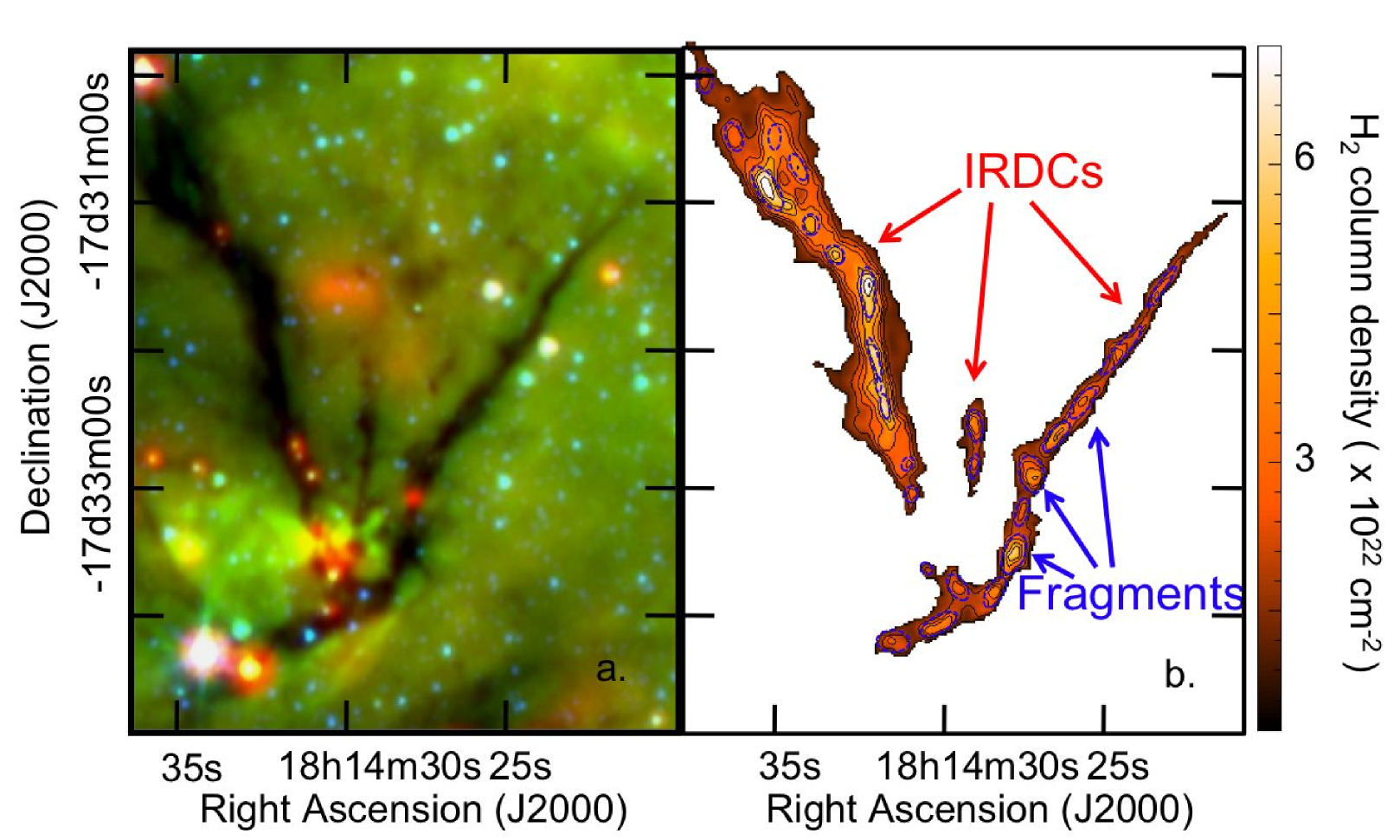
The analysed IRDCs come from a new catalogue of clouds identified in the Spitzer GLIMPSE data (PF09). IRDCs were defined as connected structures with column density peaks above cm-2 and boundaries defined by the contour at cm-2. Single peaked structures lying within the IRDCs were identified as fragments. The boundary of a fragment being defined by the contour of the local minimum between a fragment and its closest neighbour, the same criterion used to define the leaves of the dendogram analysis of Rosolowsky et al. (2008). As column density peaks, these fragments are particularly important in the context of star formation since they are the likely birth place of the future generation of stars. The catalogue includes opacity maps at 4′′ resolution and physical properties for over 11,000 IRDCs. Extracting the densest structures, a total of 50,000 fragments have been catalogued within the full sample of clouds (PF09). Figure 1a shows a Spitzer three colour image of a region containing three filamentary IRDCs from the PF09 catalogue. Figure 1b shows the column density map of these IRDCs and identifies the fragments within the clouds.

2.1 IRDC saturation
As discussed in PF09, some of the absorption towards IRDCs is saturated, meaning the infrared background is not strong enough in order to fully probe the internal structure of an IRDC. Based on photometric noise limitation and background strength PF09 estimated the fraction of saturated IRDCs to be 3%, corresponding to roughly 340 IRDCs over the entire sample.
An alternative estimate of the number of saturated clouds can be made from an inspection of the distribution of peak column density of IRDCs shown in Fig. 2. There appears to be a break in the distribution of peak at cm-2, which likely reflects the effect of saturation. The fraction of IRDCs lying above this limit is 4%, very similar to the value estimated in PF09. However, even for these saturated clouds only a small fraction of their area is above the saturation limit, only marginally affecting the averaged IRDC column density (and therefore any estimate of the cloud mass). But, the saturation has a much stronger effect on some fragments. For this reason, in the analysis presented here IRDCs containing saturated pixels are considered, but fragments with saturated pixels are excluded.
Our estimated saturation limit is roughly twice as large as the one found by Vasyunina et al. (2009) from millimetre emission in their study of particularly high column density IRDCs. The discrepancy between the low absorption column densities Vasyunina et al. determined by assuming the minimum possible foreground emission, that due to the zodical light, and the high values they determined from millimeter dust continuum led Vasyunina et al. to derive a relatively low saturation limit. However, the majority of their clouds do not in fact appear saturated as considerable substructure can be seen in the 8m extinction maps.
2.2 Column density and angular size distributions
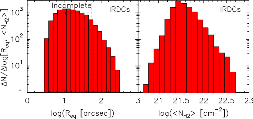
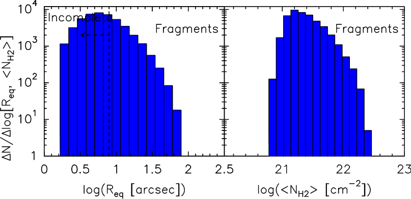
This study aims to statistically analyze the density and mass distributions of IRDCs and their fragments. To derive such quantities we first need to know the angular size and column density distributions as measured on the column density maps constructed by PF09.
Figure 3 shows the distribution of the angular size and column density for the IRDCs and the fragments identified within them. Fragments with saturated pixels have been excluded (see Sec. 2.1). In addition IRDCs which are not fragmented ( of the IRDC sample) have also been removed to maintain a clear definition of a fragment as a substructure within a cloud. However, in practice keeping these single peak clouds has little effect on the results.
It is important to note that the column densities we plot here are the background substracted column densities, equivalent to the one obtained in the clipping option of the dendogram analysis of Rosolowsky et al. (2008). In the context of centrally concentrated structures, these column densities are the relevant ones when interested in the physical properties of the gas enclosed in a given radius. Figure 3 clearly shows that the distributions are dominated by small structures of low column density. We can also clearly see the effect of incompleteness on the distributions with the decrease in the number of sources at low radius/column density, responsible for the formation of artificial peaks. The incompleteness in the sample and these distributions are discussed in Section 4.
3 IRDCs distance distribution
To calculate the density and mass of the clouds the distance of each IRDC is required, however this is not yet known for most of the 11,000 IRDCs. For this analysis we have therefore adopted a statistical approach based on previous measurements of the distances to samples of IRDCs.
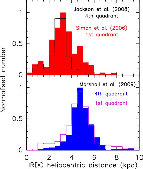
Several studies have measured the distance distribution of subsamples of IRDCs in both the 1st and 4th quadrant of the Galactic plane (Simon et al. 2006; Jackson et al. 2008; Marshall et al. 2009). Both kinematic and dust extinction techniques have been used to infer these distances, and although they lead to similar results, there are some differences (Fig. 4). The properties of these distance distributions are summarised in Table 1. Using dust extinction, Marshall et al. (2009) found a centrally peaked, Gaussian-like distance distribution very similar for both the 1st and 4th quadrant of the Galaxy (Fig. 4 - bottom panel). In a similar way, kinematic distances111These kinematic distances have been recalculated by taking the CS(2-1) and 13CO(1-0) velocities published in Jackson et al. (2008) and Simon et al. (2006), respectively, and using the Reid et al. (2009) revised galactic rotation model. shown in Fig. 4 (top panel) show a good agreement between the 1st and 4th quadrant . Although in the 1st quadrant a tail at 5 kpc clearly emerges. However most significant difference between the extinction and kinematic distances is the position of the peak, being located at kpc in one case and at kpc in the other. Both techniques have their own biases and advantages, it is therefore difficult to favor one distance distribution over another. However a Gaussian distribution is a rather good approximation to the distance distribution in both quadrants.
| Sample | Mean distance | FWHM | Dispersion, |
|---|---|---|---|
| (kpc) | (kpc) | (kpc) | |
| Marshall, 1st & 4th quad. | 4.7 | 1.5 | 1.2 |
| Jackson, 4th quad. | 3.0 | 0.8 | 1.2 |
| Simon,1st quad. | 3.6 | 2.5 | 1.3 |
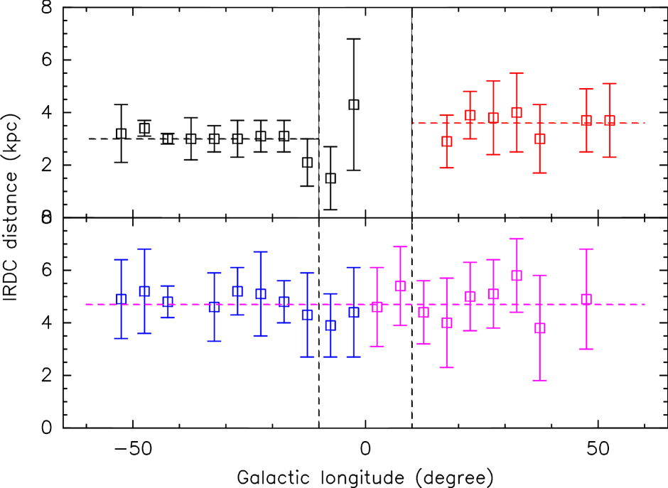
Fig. 4 (right) shows the average distance to the IRDCs as a function of galactic longitude for the sources with distances measured by these two techniques. Any systematic trend with longitude could introduce a bias in analysis adopting a statistical distribution for the distance of IRDCs. It is clear that there is very little variation of the IRDC distances with respect to the galactic longitude. The only region where there may be such an effect is towards galactic centre seems, an area which is not covered in our IRDC Spitzer catalogue which only extends into . It is worth noting that distance variations around the mean as a function of longitude are very similar for both methods, emphasising that is it predominantly only the average distance which differs between the two methods.
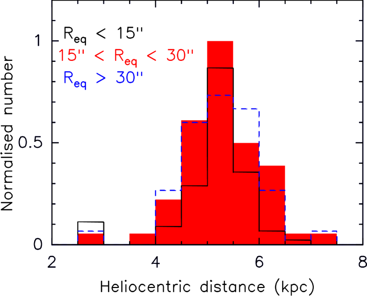
Another possible bias is with respect to the size of the IRDCs. The studies shown in Fig. 4 do not contain IRDCs as small as those in the Spitzer based sample and so it is possible that the small and large clouds have different distance distributions. However, recent observations with ATNF Mopra in CS J=1-0 (Peretto et al. in prep) of a square degree of the galactic plane (, ) can be used to investigate this possibility. This area covers 196 Spitzer IRDCs in total and more than 80 of the clouds can be associated with CS emission.
The distances of these clouds can be calculated using the Reid et al. (2009) galactic rotation model. Figure 5 shows the distance distribution of the Spitzer IRDCs detected in CS. In this figure, the IRDCs have been divided int to three size ranges. The 80 smallest IRDCs, those with (PF09) less than 15′′ have a mean distance and standard deviation of kpc and kpc. This is indistinguishable from the values of kpc and kpc and kpc and kpc for the IRDCs in the next two size ranges, , , which contain and objects respectively. These distributions therefore show no indication that large and small IRDCs have different distributions of distance.
4 Completeness limits
4.1 Column Density and Mass
The mass completeness limit for the IRDCs and fragments can be written as
| (1) |
where is the smallest radius above which the sample is complete, is the distance within which the majority of the sources occur, and is the typical average column density of the structures with a radius . Figure 4(left) shows that about 95 of the IRDCs in that plot have distances below 6 kpc and so we conservatively adopt kpc.
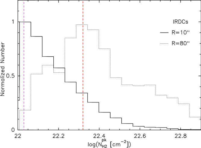
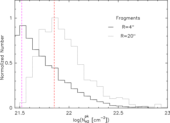
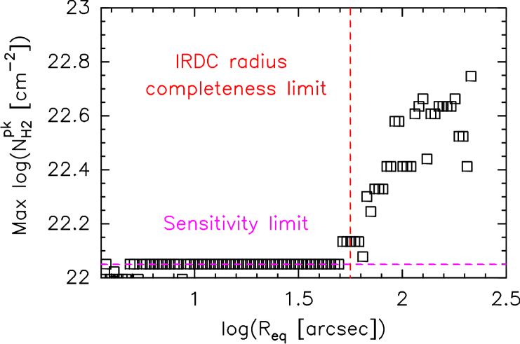
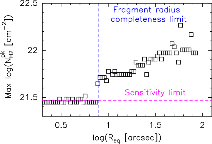
Estimating is less straighforward. The completeness limits of our survey are related to two parameters of the source extraction: , the minimum column density amplitude of a source (which is related to sensitivity) from the boundary of a cloud to its peak; and the angular resolution, 4′′ both for IRDCs and fragments. In order to investigate how these contribute to the completeness limits we look at the distribution of average column density of IRDCs for objects of a given range of sizes as plotted in Fig. 6. We then plot the column density at the peak of these distributions as a function of cloud size. This is also done for the fragments. Figure 7 shows these plots.
The plots show a similar structure for both the IRDCs and fragments. Up to some size, for the IRDCs and for the fragments, the peak of the column density distributions is constant. Above these values it increases with increasing size. This constant column density for small sizescales suggests that the sample is not fully probing the populations of objects at these sizescales. There are objects in these size ranges which have lower column densities and are not sampled by the objects in the catalogue. These plots therefore show the size limit completeness of the catalogue, for both IRDCs, , and fragments, .
Adopting these sizes, the average column density of clouds/fragments below these sizes gives average column density completeness limits of cm-2 and cm-2. Using Eq. 1, these values give the mass completeness of the catalogue as M⊙ and M⊙.
4.2 Density
The density distribution of IRDCs is difficult to interpret since the clouds are defined based on a column density threshold. Therefore we confine our discussion of the density distributions to the fragments. Both sensitivity and angular resolution are important limiting factors in the context of density completeness of the sample: both compact low-mass fragments and large, diffuse, high-mass fragments could remain undetected. For any fragment mass, there is a minimum radius for which the peak column density of the fragment becomes higher than the threshold for identifying fragments (cm-2). If this minimum radius is larger than the angular resolution then such a fragment is detected. Therefore, we can define a density completeness limit for all fragments more massive than . The minimum radius, , and the corresponding maximum density, , are given by
| (2) | |||||
| (3) |
where is the mean mass per molecule and we adopt a column density which is the average column density of fragments of mass (which by definition have peak column densities greater than the threshold to be identified as fragments). At a distance of 6 kpc, for fragment mass of 2/8/32 M⊙ and cm-2 we get R′′ and cm-3, respectively.
For the same given mass there is also an upper density limit which corresponds to the point where the size of the fragment becomes smaller than the resolution of the observations. This provides an upper limit on the density, . For the 3 masses discussed before we get cm-3.
5 Size, mass and density structure of IRDCs
5.1 Physical size distribution
To calculate the density and mass of the IRDCs and fragments requires a distance for each object. Two different approaches to statistically attribute a particular distance to a particular cloud have been adopted. The first is to simply assign a unique distance to all clouds. Doing this, the physical size distribution of IRDCs and fragments will be exactly the same as the angular size distribution. Given the well peaked distribution of distances for clouds with measured distances (Fig. 4), this should be a reasonable first approximation. However, a more sophisticated approach is to make use of the distribution of distances (rather than just its peak position). To do this we adopt a distance distribution for the IRDCs and then randomly assign a distance drawn from this distribution to each cloud. Doing this for the whole sample of clouds repeatedly provides a statistical sampling of the distance distribution. The final physical size distribution is the convolution of the true physical size distribution by the chosen distance distribution. However this does not have a crucial impact on the interpretation of the physical size distribution if the dispersion of the distance distribution is much smaller than the angular size distribution. This is clearly the case since the angular sizes, both for IRDCs and fragments, extends over 2 order of magnitudes while IRDC distances span only over a factor of 3 at most. In other words, the dispersion in distance has relatively little effect on the final physical size distribution (see Appendix A). To assign distances to the clouds using this sampling technique we adopt a Gaussian distribution of distances with a peak at 4 kpc and a dispersion of 1 kpc, consistent with observed distance distributions (Fig. 4).
5.2 Mass distributions
Mass distributions of molecular cloud structures have been extensively studied in the past, therefore they represent a good point of comparison for this current study. We defined mass as:
| (4) |
where is the average column density across the IRDC or fragment and its equivalent radius (PF09).
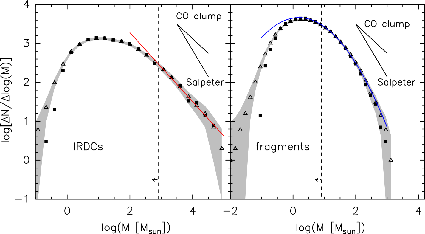
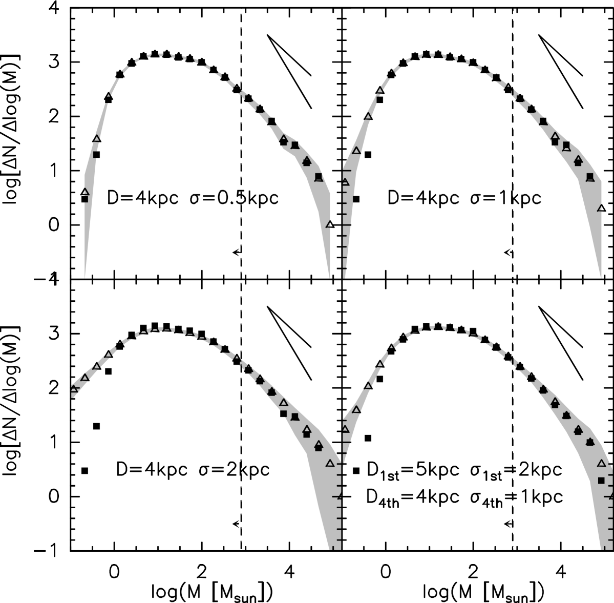
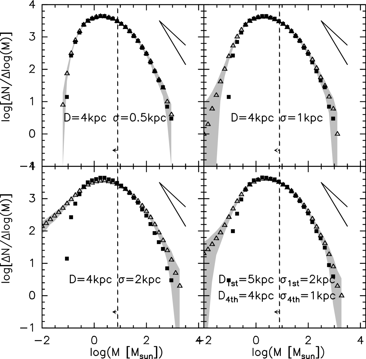
Figure 8 shows the mass distributions for IRDCs and fragments calculated adopting a single distance of 4kpc (filled square symbols) and for randomly attributed distances as described in Section 5.1. The shaded band on the figures shows the range (3 times the dispersion) spanned by the 100 different distance realizations and the open triangles the mean for the different realizations. The completeness limits are shown by the dashed lines. For comparison the power-law slopes of the CO clump mass function (slope ) and the Salpeter mass function (slope ) are also shown. Using the MPFITS IDL package (Markwardt 2009) we have fitted the two distributions above their respective completeness limits. For the IRDCs we find a linear function (in a log-log plot) provides a good fit with with . The mass distribution of fragments is better fitted by a lognormal function defined as
| (5) |
where A is a normalization constant, is the peak mass of the distribution, and is the dispersion. However, since we do not map the peak, the precise parameters of the lognormal function fit are not well constrained, several provide adequate fits to the data points. The function showed in Fig. 8 has A=4610, M M⊙, and . As argued above, the figure confirms that as a consequence of the nature of the distance distribution, there is relatively little difference in the derived mass distributions whether a single distance is adopted for the clouds or statistical approach is adopted. Also, the results of this analysis are also not strongly dependent on exact parameters of the assumed distance distribution as demonstrated in Appendix A.
A number of previous studies have attempted to construct, with samples at least an order of magnitude smaller, the mass distributions of IRDCs (Simon et al. 2006; Marshall et al. 2009) and fragments within them (Rathborne et al. 2006; Ragan et al. 2009). Except for the Ragan et al. study, the mass distributions in these studies agree: the IRDC mass distribution is similar to that of CO clumps, while the distribution for the sub-structures are steeper, more like the Salpeter IMF.
In their analysis of 11 IRDCs, Ragan et al. (2009) found that the mass distributions of what they called clumps, which correspond to fragments here, is quite flat, similar to the CO clump mass distribution, in contrast with the present study. However it is difficult to understand the Ragan et al. result as the radii and masses they quote for their clumps imply 8µm opacities over 10 times larger than the 8µm opacities they quote.
5.3 Density distribution
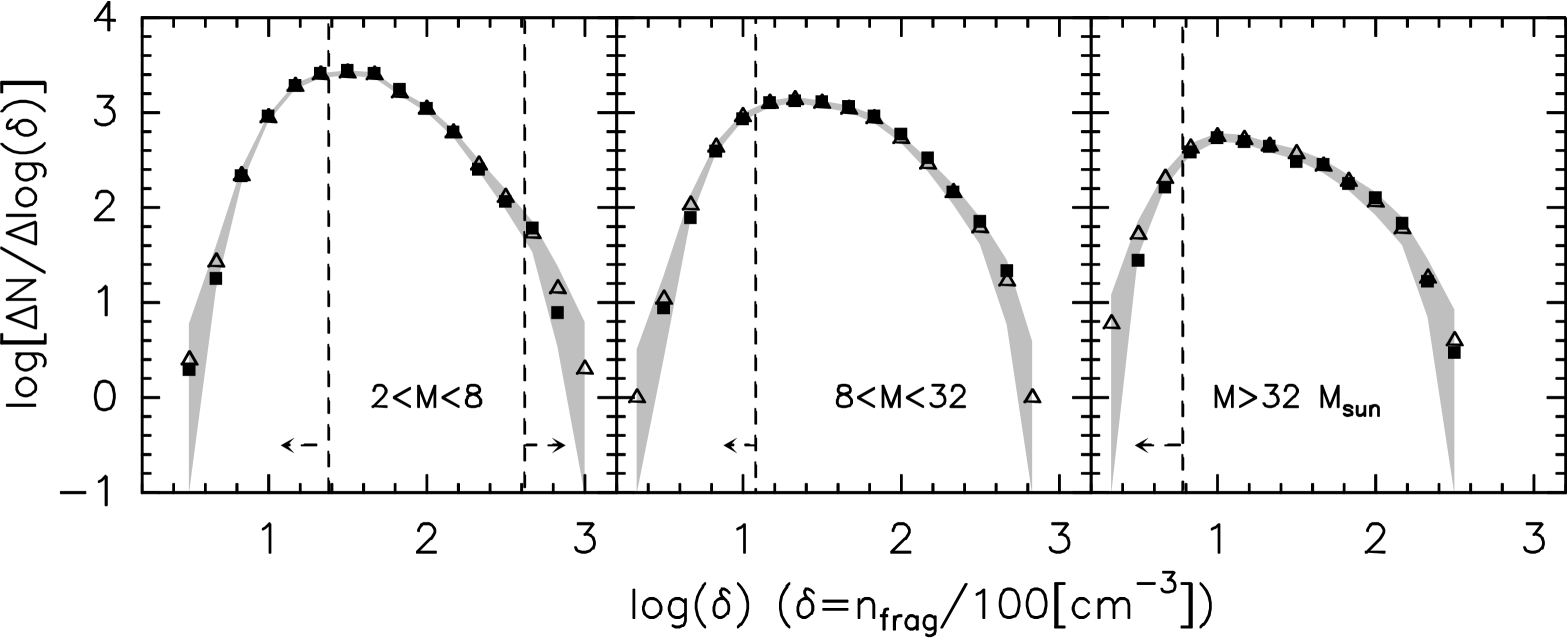
The density distribution of fragments may provide important insights on the physical process generate these structures. We define the number density of a fragment as
| (6) |
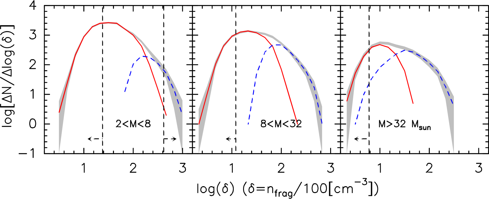
where dt is the line of sight size of the fragments which is assumed to be twice the projected radius. Figure 9 shows the fragment density distributions for the following mass ranges: M⊙, M⊙ and M⊙. For each range, the density completeness limit, the dashed line, is calculated for M⊙, respectively. The density distribution over the entire mass range is very similar to that for the lower mass range (left panel). The figures show that going from low mass to high mass fragments, the distributions become flatter. Compared to low density fragments, there is a higher probability of finding high density fragments for high mass fragments. One of the main issue in interpreting such a plot in terms of the formation of the fragments is that the density of gravitationally bound fragments is increasing over the time as they evolve (i.e. contract), and therefore might pollute the initial density PDF of the parental IRDCs. In the next section we will discuss the impact of such effects on the density distributions.
6 Discussion: Turbulent vs gravitational dominated structures
The mass distributions of IRDCs and fragments plotted in Fig. 8 clearly shows a steepening, from large structures to smaller fragments. While the mass distribution of IRDCs is similar to that of CO clumps, the fragment mass distribution has a slope at high masses which is reminiscent of the slope of the Salpeter IMF, although it is best fitted with a lognormal function. However, two biases could affect the shape of the high-mass end of the distribution and the interpretation that its slope is related to the Salpeter IMF. The detailed structure of this part of the distribution may be particularly sensitive to the adopted Gaussian distance distribution. Also high-mass fragments might evolve more rapidly than their low-mas analogues and therefore be under represented in extinction observations at 8m (c.f. Hatchell & Fuller 2008).
To the first order, the mass distributions are in agreement with the theoretical work of Hennebelle & Chabrier (2008) who interpreted the transition from a flat mass distribution to a steeper one as the transition from turbulence-generated structures to gravity dominated structures. In this context it is interesting to measure the gravitational binding of IRDCs and fragments. To investigate this, we have used Larson’s relation (Larson 1981) to compute the kinetic support, and calculate the virial mass. Following Hennebelle & Chabrier (2008) we assume the effective velocity dispersion is given by
| (7) |
where is the sound speed is the normalization velocity of Larson’s relation, is the power law index of Larson’s relation, and is the size of the structure. We can then use this to compute the corresponding virial mass Mvir for every IRDC/fragment. Figure 10 shows the fraction of IRDCs and fragments having a ratio , assuming km/s (T=10 K), km/s, and . Above the completeness limit all the IRDCs appear gravitationally bound, as do the majority of the fragments. Of course large uncertainties exist on the use of Larson’s relation and its normalization. However, different normalizations still give similar conclusions about the fraction of IRDCs and fragments which are bound.
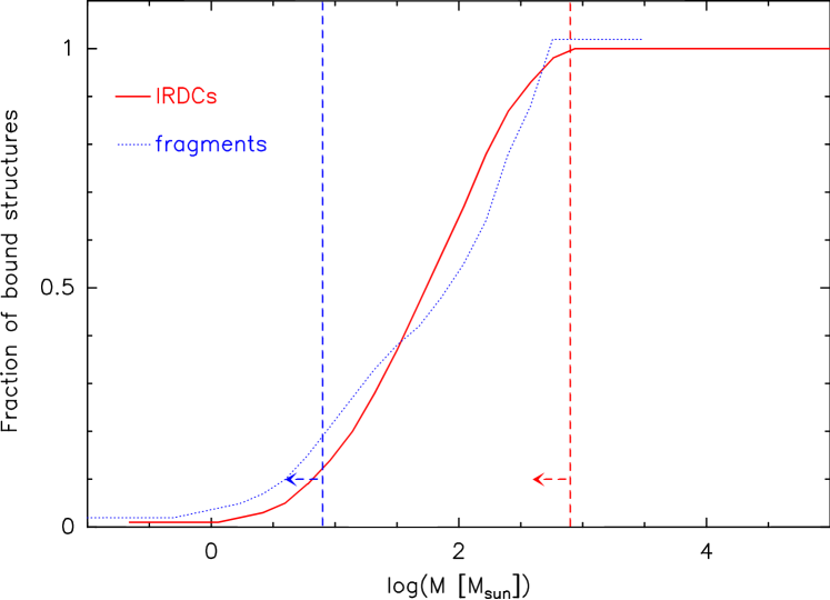
A consequence of the IRDCs being gravitationally bound is that the observed change of slope of the mass distributions shown in Fig. 8 does not represent the transition from turbulence dominated to gravity dominated structures: most of the IRDCs down to the completion limit are bound. However, as shown in Fig. 10 a significant fraction of the fragments lying above the completeness limit are unbound. In other words, even if globally gravitationally bound, IRDCs may contain turbulence-generated over-densities which will probably disperse and not form stars. The physical properties of these unbound fragments are likely to be representative of the initial conditions of star formation within IRDCs.
Using the previously defined ratio to separate bound fragments to unbound ones we constructed the density distributions for both type of fragments as shown in Fig. 11. The mass ranges are the same as in Fig. 9. The unbound fragments have all very similar distributions, independent of their mass range. In particular, the high mass end of the distribution is well fit by the following relation , the error bar arising from the uncertainties on Larson’s relation. The location of the peak seems to move with the completeness limit and is therefore questionable. From these plots we cannot exclude a possible lognormal distribution for unbound fragments, but the peak of such distribution would have to be below n cm-3.
In contrast, the density distribution of the gravitationally bound fragments show a well defined peak between n= cm-3 and cm-3 in each mass range and a shape which broadens to lower densities as the mass range increase. This could result from the higher mass fragments of a given density evolving to being bound more rapidly that lower mass fragments.
7 Summary
We used the largest sample of IRDC column density maps to date in order to better characterize the size, mass, and density structure of dense molecular clouds. The large number of objects, 11,000 IRDCs and 50,000 fragments, allows a detailed analysis of the completeness of the sample. Using a statistically attribute distances to each IRDC, we have demonstrated that above the completeness limit the mass distribution of the IRDCs are consistent with a power-law , where is the number of clouds. For the fragments the high mass end of the mass distribution shows a steeper slope, consistent with the slope of the Salpeter IMF, with the overall distribution well fitted by a lognormal function.
Using Larson’s law to estimate the linewidth of each IRDC and fragment, we have shown that above our completeness limit all the IRDCs and the majority of fragments are likely to be bound. This implies that the transition in the shape of the mass distribution does not reflect a transition from unbound to graviationally bound structures. Looking at the distribution of fragment density shows that bound fragments dominate the high density ( cm-3) end of the distribution for all mass ranges, and dominate the whole distribution for the highest range of fragment masses. There is also a distinct broadening of the distribution with increasing fragment mass. This could be a result of the higher mass fragments evolving to being bound more rapidly that lower mass fragments. The number of unbound fragments as a function of number density has the form (where is the number of fragments) down to a density of cm-3 where the completeness limit is reached.
The absence of bright infrared sources embedded in IRDCs indicates that the mass distributions and density distributions as a function of mass and degree of gravitational binding derived here are representative of the initial conditions of star formation within dense molecular clouds. These results should serve as constraints on theoretical and numerical models in order to identify and characterize the physical processes responsible for the formation and early fragmentation of molecular clouds.
Appendix A Different distance distributions
In order to investigate further the impact of choosing a given distance distribution on the calculated mass distributions we performed a series of tests with different assumptions. Using the same approach as described in Section 4 and 5, we used a Gaussian distribution for distances with a mean distance of 4 and 5 kpc with dispersions of 0.5, 1 and 2 kpc. We also performed a test assuming different distance distributions for the 1st quadrant and 4th quadrant IRDCs. We show the resulting mass distributions in Fig. 12 and 13. We see that the shape of the mass distributions above the completeness limits for both the IRDCs and fragments, remain basically the same, with best fit parameters changing only of a few 0.1 dex.
References
- Buckle et al. (2010) Buckle, J. V., et al. 2010, MNRAS, 401, 204
- Chabrier (2003) Chabrier, G., 2003 in IAU Symposium, Vol. 221, IAU Symposium, 67P-+
- Dring et al. (1996) Dring, A. R., Murthy, J., Henry, R. C., & Walker, H. J. 1996, ApJ, 457, 764
- Enoch et al. (2008) Enoch, M. L., Evans, II, N. J., Sargent, A. I., et al. 2008, ApJ, 684, 1240
- Hatchell & Fuller (2008) Hatchell, J. & Fuller, G. A. 2008, A&A, 482, 855
- Hennebelle & Chabrier (2008) Hennebelle, P. & Chabrier, G. 2008, ApJ, 684, 395
- Jackson et al. (2008) Jackson, J. M., Finn, S.C., Rathborne, J. M., Chambers, E., T., Simon, R., 2008, ApJ, 680, 349
- Kramer et al. (1998) Kramer, C., Stutzki, J., Rohrig, R., Corneliussen, U. 1998, A&A, 329, 249
- Larson (1981) Larson, R. B. 1981, MNRAS, 194, 809
- Markwardt (2009) Markwardt, C. B. 2009, Astronomical Society of the Pacific Conference Series, 411, 251
- Marshall et al. (2009) Marshall, D.J., Joncas, G., Jones, A., P., 2009, ApJ, 706, 727
- Motte et al. (1998) Motte, F., André, P., Neri, R. 1998, A&A, 336, 150
- Padoan et al. (1997) Padoan, P., Nordlund, A., Jones, B. J. T. 1997, MNRAS, 288, 145
- Perault et al. (1996) Perault, M., et al. 1996, A&A, 315, L165
- Peretto & Fuller (2009) Peretto, N. & Fuller, G. A., 2009, A&A, 505, 405
- Pineda et al. (2009) Pineda, J. E., Rosolowsky, E. W., & Goodman, A. A. 2009, ApJ, 699, L134
- Ragan et al. (2009) Ragan, S. E., Bergin, E. A., & Gutermuth, R. A. 2009, ApJ, 698, 324
- Rathborne et al. (2006) Rathborne, J. M., Jackson, J. M., & Simon, R. 2006, ApJ, 641, 389
- Reid et al. (2009) Reid, M.J., Menten, K.M., Zheng, X.W. et al., 2009, ApJ, 700, 137
- Reid & Wilson (2006) Reid, M. A., & Wilson, C. D. 2006, ApJ, 644, 990
- Rosolowsky (2004) Rosolowsky, E. 2004, Bulletin of the American Astronomical Society, 36, 1470
- Rosolowsky et al. (2008) Rosolwsky, E. W., Pineda, J.E., Kauffmann, J., Goodman, A. A., 2008, ApJ, 679, 1338
- Simon et al. (2006) Simon, R., Rathborne, J. M., Shah, R. Y., Jackson, J. M. & Chambers, E. T. 2006, ApJ, 653, 1325
- Smith & Scalo (2009) Smith, D. S., & Scalo, J. M. 2009, Astrobiology, 9, 673
- Teyssier et al. (2002) Teyssier, D., Hennebelle, P., & Pérault, M. 2002, A&A, 382, 624
- Vasyunina et al. (2009) Vasyunina, T., Linz, H., Henning, T., et al., 2009, A&A, 499, 149