A Statistically Principled and Computationally Efficient Approach to Speech Enhancement using Variational Autoencoders

A common approach to modeling sound sources is to assume the short time Fourier Transform (STFT) coefficients are proper complex Gaussian random variables. With $f$ denoting the frequency index and $t$ the time-frame index, for all $(f,t)\in\{0,...,F-1\}\times\{0,...,N-1\}$, each source STFT coefficient $s_{ft}\in\mathbb{C}$ independently follows

Several frameworks have been used to model the variance $\sigma^{2}_{ft}$ of this distribution [20, 2]. To this end, we choose to use the VAE framework, which uses the representational power of DNNs to build generative models. It consists in mapping a zero-mean unit Gaussian random variable $\mbox{\boldmath$z$}_{t}\in\mathbb{R}^{L}$ through a DNN, into the desired output distribution. In our setting, we use it to represent $\sigma^{2}_{ft}$. The generative model can be written as

where $\sigma_{f}^{2}:\mathbb{R}^{L}\mapsto\mathbb{R}_{+}$ is a non-linear function implemented by a DNN with parameters $\theta$. Each $\sigma_{f}^{2}$ is one neuron of a F-dimensional output layer of a single DNN.

The VAE is trained on clean speech data by maximizing the likelihood $p_{\theta}(\mbox{\boldmath$s$})=\prod_{t}p_{\theta}(\mbox{\boldmath$s$}_{t})$, with $\mbox{\boldmath$s$}_{t}=\left[s_{1t},...,s_{Ft}\right]^{T}$. To do so, we introduce a variational approximation of $p_{\theta}(\mbox{\boldmath$z$}_{t}|\mbox{\boldmath$s$}_{t})$ , $q_{\phi}(\mbox{\boldmath$z$}_{t}|\mbox{\boldmath$s$}_{t})$, parametrized by $\phi$. We have

where $\mathcal{D}_{KL}(q||p)=-\mathbb{E}_{q}[\log(p/q)]$ denotes the Kullback-Leibler (KL) divergence. The KL term on the left hand side of (4) being always positive, $\mathcal{L}(\mbox{\boldmath$\theta$},\mbox{\boldmath$\phi$};\mbox{\boldmath$s$}_{t})$ is a lower bound of the marginal log-likelihood $\log p_{\theta}(\mbox{\boldmath$s$}_{t})$. We can thus maximize the individual $\mathcal{L}(\mbox{\boldmath$\theta$},\mbox{\boldmath$\phi$};\mbox{\boldmath$s$}_{t})$ with respect to $\theta$ and $\phi$ in order to maximize the log-likelihood $\log p_{\theta}(\mbox{\boldmath$s$})$. For all $(l,t)\in\{0,...,L-1\}\times\{0,...,N-1\}$, $q_{\phi}(z_{lt}|\mbox{\boldmath$s$}_{t})$ is defined as in [8]

where $\tilde{\mu}_{l}$ and $\tilde{\sigma}_{l}^{2}$ are DNN-based functions parametrized by $\phi$. Finally, we can use (2), (3) and (6) to write (5) as

where $d_{IS}(x,y)=x/y-\log(x/y)-1$ denotes the Itakura-Saito divergence, $\mbox{\boldmath$z$}_{t}=\left[z_{1t},...,z_{Lt}\right]^{T}$ and $\overset{c}{=}$ denotes equality up to a constant. Using the so-called reparametrization trick [16], we can maximize $\mathcal{L}(\mbox{\boldmath$\theta$},\mbox{\boldmath$\phi$};\mbox{\boldmath$s$})$ using gradient descent optimization algorithms [21].

The variational distribution $q_{\phi}(\mbox{\boldmath$z$}_{t}|\mbox{\boldmath$s$}_{t})$ is usually considered as an unwanted by-product of the training procedure of the VAE, only introduced to learn $p_{\theta}(\mbox{\boldmath$s$}_{t}|\mbox{\boldmath$z$}_{t})$. However, by examining carefully (4), we can see that while maximizing $\mathcal{L}(\mbox{\boldmath$\theta$},\mbox{\boldmath$\phi$};\mbox{\boldmath$s$}_{t})$ can only increase the log-likelihood, it also decreases the KL divergence between the true posterior and its variational approximation. In other words, in addition to the generative speech model, the VAE provides a variational approximation of the true posterior. This feature will play a key role in the inference algorithm proposed in Section 3.

As in [8], the STFT coefficients $n_{ft}$ of the noise are modelled with a rank-$K$ NMF Gaussian model. For all $(f,t)$

with $\mbox{\boldmath$W$}\in\mathbb{R}_{+}^{F\times K}$, $\mbox{\boldmath$H$}\in\mathbb{R}_{+}^{K\times N}$.

Finally, independently for all $(f,t)$, the single-channel observation of the noisy speech is modeled by

where $s_{ft}$ and $n_{ft}$ are independent.

We define $\sigma^{2}_{n,ft}=(\mbox{\boldmath$W$}\mbox{\boldmath$H$})_{ft}$ to make the notation less cluttered. Using (12), we find (see [22])

where $\mbox{\boldmath$\mu$}_{ft}$ and $\mbox{\boldmath$\Sigma$}_{ft}$ are defined as

with

where $\{\mbox{\boldmath$z$}_{n}^{(d)}\}_{d=1,..,D}$ are randomly drawn from $r(\mbox{\boldmath$z$}_{t})$.

We note $[\mbox{\boldmath$\mu$}_{s,t},\mbox{\boldmath$\mu$}_{n,t}]=\mbox{\boldmath$\mu$}_{t}$ and define $\mbox{\boldmath$\Sigma$}_{ss,t}$ and $\mbox{\boldmath$\Sigma$}_{nn,t}$ to be the diagonal terms of $\mbox{\boldmath$\Sigma$}_{t}$.

We can compute $r(\mbox{\boldmath$z$}_{t})$ using (13) (see [22]), we get

where (18) was obtained using Bayes’ theorem. The VAE assumes that $p_{\theta}(\mbox{\boldmath$z$}_{t}|\mbox{\boldmath$s$}_{t})$ can be appproximated by $q_{\phi}(\mbox{\boldmath$z$}_{t}|\mbox{\boldmath$s$}_{t})$. We further assume that this still holds for $\mbox{\boldmath$s$}_{t}$ of the form $\left(|\mbox{\boldmath$\mu$}_{s,t}|^{2}+\mbox{\boldmath$\Sigma$}_{ss,t}\right)^{\frac{1}{2}}$. That is to say

We now maximize $\mathcal{L}(r,\mbox{\boldmath$\Theta$}_{t})$ with respect to $\mbox{\boldmath$\Theta$}_{t}$ using (14). With $\mbox{\boldmath$V$}\in\mathbb{R}_{+}^{F\times N}$ defined as $(\mbox{\boldmath$V$})_{t}=|\mbox{\boldmath$\mu$}_{n,t}|^{2}+\mbox{\boldmath$\Sigma$}_{nn,t}$, and $\odot$ denoting element-wise matrix multiplication and exponentiation, we obtain multiplicative updates as in [23]:

Let $\mbox{\boldmath$\Theta$}^{\star}=\{\mbox{\boldmath$W$}^{\star},\mbox{\boldmath$H$}^{\star}\}$ and $r^{\star}(\mbox{\boldmath$s$},\mbox{\boldmath$b$},\mbox{\boldmath$z$})=r^{\star}(\mbox{\boldmath$s$},\mbox{\boldmath$b$})r^{\star}(\mbox{\boldmath$z$})$ be respectively the set of NMF parameters and the variational distribution estimated by the proposed algorithm. The final estimate of the source is given, as in [8], by

There are three ways to evaluate this estimate. The straightforward way is to replace $p(s_{ft}|x_{ft};\mbox{\boldmath$\Theta$}^{\star})$ in (23) by its variational approximation $r^{\star}(s_{ft})$. The expectation over $p(\mbox{\boldmath$z$}_{t}|x_{ft};\mbox{\boldmath$\Theta$}^{\star})$ can also be approximated using the Metropolis Hastings (MH) algorithm as in [8], using the mean of $r^{\star}(\mbox{\boldmath$z$}_{t})$ as the initial sample. And finally we can compute the expectation in (24) by replacing $p(\mbox{\boldmath$z$}_{t}|x_{ft};\mbox{\boldmath$\Theta$}^{\star})$ by its variational approximation $r^{\star}(\mbox{\boldmath$z$}_{t})$. We will respectively refer to these methods as S-Wiener, MH-Wiener and Z-Wiener for ease of referencing.
Metropolis-Hastings : At the $m$-th iteration of the Metropolis-Hastings algorithm, we draw a random sample for each $t$ according to

The acceptance probability can be computed as

We accept the new sample and set $\mbox{\boldmath$z$}^{(m)}_{t}=\mbox{\boldmath$z$}_{t}$ only if $u$, drawn from a uniform distribution $\mathcal{U}([0,1])$, is smaller than $\alpha$. We keep only the last $R$ samples to compute $\hat{s}_{ft}$ from (24) and discard the samples drawn during the burn-in period.

Dataset: As in [8, 9], we use the the TIMIT corpus [24] to train the clean speech model. At inference time, we mix speech signals from the TIMIT test set with noise signals from the DEMAND corpus [25] at 0dB signal-to-noise ratio, according to the file provided in in the original implementation of [8] ¹¹1https://gitlab.inria.fr/sileglai/mlsp2018. Note that both speakers and utterances are different from those in the training set.

VAE’s architecture and training: The architecture of the VAE is the same as in [8]. The hyperbolic tangent of an input 128-dimensional linear layer passes through two L-dimensional linear layers to estimate $\tilde{\mu}_{l}({|\mbox{\boldmath$s$}_{t}}|^{2})$ and $\log\tilde{\sigma}_{l}^{2}({|\mbox{\boldmath$s$}_{t}|^{2}})$, from which $\mbox{\boldmath$z$}_{t}$ is sampled using the reparametrization trick. $\mbox{\boldmath$z$}_{t}$ is then fed to a 128-dimensional linear layer with hyperbolic tangent activation followed by an linear output layer predicting $\log\sigma_{f}^{2}(\mbox{\boldmath$z$}_{t})$. For training, we computed the STFT of the utterances with a 1024-points sine window and a hop size of 256 points. 20$\%$ of the training set is held for validation. A VAE with $L=64$ is trained with the Adam optimizer [26], using a learning rate of $10^{-3}$ and a batch size of 128. Training stops if no improvement is seen on the validation loss for 10 epochs.

Baseline methods: We compare our method to two baselines. The first baseline, developed in [8], shares the same statistical assumptions made in Section 2 except for the inclusion of a gain factor in (9). The inference is performed using a Monte Carlo Expectation-Maximization (MCEM) algorithm in which MH sampling is used to estimate the true posterior. We will refer to this method as MCEM. The second baseline is a heuristic we introduce to evaluate the impact of the covariance term $\mbox{\boldmath$\Sigma$}_{ss,t}$ in (20) on the convergence of the algorithm. We simply remove $\mbox{\boldmath$\Sigma$}_{ss,t}$ from (20) and the rest of the algorithm remains unchanged. Note that this is similar to the heuristic developped in [15] for determined multichannel source separation, only adapted to single-channel speech enhancement.

Inference Setting: For fair comparaison, we use the same settings for the three methods : the rank of the NMF model is set to $K=10$, the latent dimension of the VAE is set to $L=64$ and the same stopping criterion is used as in [8]. $\mbox{\boldmath$z$}_{t}$ is initialized based on $q_{\phi}(\mbox{\boldmath$z$}_{t}|\mbox{\boldmath$x$}_{t})$ and for the final speech estimate, equation (24) is approximated using the last 25 samples of a 100-iteration MH sampling with $\epsilon^{2}=0.01$. In [8], for $R$ samples used, the total number of draws is $4R$. The methods will be compared for a same number of samples actually used to estimate the expected values : if $D$ samples are used to evaluate (17), $4D$ samples will be drawn in the MCEM case.

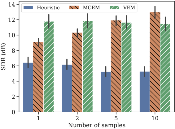
Experiment 1: We first compare the performances of the three methods on the test set described above, in terms of Signal to Distorsion Ration (SDR) [27], computed using the mir_eval²²2https://github.com/craffel/mir_eval toolbox. The comparison is done for different numbers of samples $D\in\{1,2,5,10\}$. As can be seen in Fig. 1, the heuristic algorithm consistently performs worse than both other methods, proving the importance of the covariance term $\mbox{\boldmath$\Sigma$}_{ss,t}$ in (20). We also see that the performances of the proposed algorithm do not depend on the number of samples drawn to approximate (17), contrary to the MCEM algorithm which presents poor performances for $R=1$ and outperforms the proposed method for $R=10$. The superiority of the MCEM algorithm for a large number of samples is not surprising due to the approximation involved in the VEM approach.

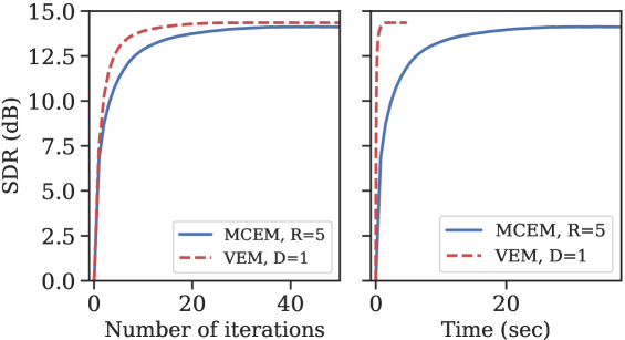
Experiment 2: We then compare the SDR achieved by the MCEM and VEM methods as a function of the computational time, in terms of number of iteration and absolute time. The number of samples $D$ was set to 1 for the VEM, and $R$ to 5 for the MCEM so as to achieve a similar SDR at convergence (see Fig. 1). At each iteration of both methods, we estimate the speech spectra by approximating (24) with MH sampling and we compute the SDR. This is done for each test utterance. Each individual SDR curve is then padded with the SDR obtained at the last iteration and all SDR curves are averaged to produce the left graph in Fig. 2. We observe that the proposed method converges faster which suggests that using the encoder allows for bigger jumps in the latent space than the sampling method with a small number of samples. On a 4-core i7-8650U CPU, one iteration takes on average 55 ms and 753 ms for the VEM and the MCEM algorithm respectively. Using these numbers, we can convert the SDR as a function of the number of iterations to the SDR as a function of time. This is shown in the right part of Fig. 2 where the superiority of the proposed algorithmm in terms of absolute speed is clear. To compare the execution times, for each utterance and for both algorithms we compute the number of iteration needed to reach the final SDR up to 0.5dB tolerance. The ratio between the number of iterations multiplied by the time per iteration ratio yields an average computational cost decrease factor of 36 to reach the same performance.

Experiment 3: In this experiment, we compare the three different ways of computing the source STFT coefficients in (23). We present the mean SDR after convergence for the three possible methods in Table 1. We can see that MH sampling consistently outperforms the other methods, suggesting that a better posterior approximation benefits to the quality of the reconstruction.

References

- [1] P. C. Loizou, Speech Enhancement: Theory and Practice, 2nd ed. Boca Raton, FL, USA: CRC Press, Inc., 2013.
- [2] E. Vincent, T. Virtanen, and S. Gannot, Audio Source Separation and Speech Enhancement. Wiley, Aug. 2018.
- [3] F. Weninger, J. R. Hershey, J. L. Roux, and B. W. Schuller, “Discriminatively trained recurrent neural networks for single-channel speech separation,” 2014 IEEE Global Conference on Signal and Information Processing (GlobalSIP), pp. 577–581, 2014.
- [4] J. R. Hershey, Z. Chen, J. Le Roux, and S. Watanabe, “Deep clustering: Discriminative embeddings for segmentation and separation,” 2016 IEEE International Conference on Acoustics, Speech and Signal Processing (ICASSP), Mar 2016.
- [5] X. Lu, Y. Tsao, S. Matsuda, and C. Hori, “Speech enhancement based on deep denoising autoencoder,” in INTERSPEECH, 2013.
- [6] A. A. Nugraha, A. Liutkus, and E. Vincent, “Multichannel audio source separation with deep neural networks,” IEEE/ACM Transactions on Audio Speech and Language Processing, vol. 24, no. 9, pp. 1652–1664, 2016.
- [7] A. Ozerov and C. Fevotte, “Multichannel nonnegative matrix factorization in convolutive mixtures for audio source separation,” IEEE Transactions on Audio, Speech and Language Processing, vol. 18, no. 3, pp. 550–563, 2010.
- [8] S. Leglaive, L. Girin, and R. Horaud, “A variance modeling framework based on variational autoencoders for speech enhancement,” in Proc. IEEE Int. Workshop on Machine Learning for Signal Processing (MLSP), 2018.
- [9] S. Leglaive, U. Simsekli, A. Liutkus, L. Girin, and R. Horaud, “Speech enhancement with variational autoencoders and alpha-stable distributions,” in IEEE International Conference on Acoustics Speech and Signal Processing (ICASSP). Brighton, United Kingdom: IEEE, 2019, pp. 1–5.
- [10] Y. Bando, M. Mimura, K. Itoyama, K. Yoshii, and T. Kawahara, “Statistical speech enhancement based on probabilistic integration of variational autoencoder and non-negative matrix factorization,” in 2018 IEEE International Conference on Acoustics, Speech and Signal Processing (ICASSP). IEEE, apr 2018, pp. 716–720.
- [11] S. Leglaive, L. Girin, and R. Horaud, “Semi-supervised multichannel speech enhancement with variational autoencoders and non-negative matrix factorization,” no. 3, 2018.
- [12] K. Sekiguchi, Y. Bando, K. Yoshii, and T. Kawahara, “Bayesian Multichannel Speech Enhancement with a Deep Speech Prior,” Apsipa, no. November, pp. 1233–1239, 2018.
- [13] H. Kameoka, L. Li, S. Inoue, and S. Makino, “Semi-blind source separation with multichannel variational autoencoder,” aug 2018.
- [14] S. Seki, H. Kameoka, L. Li, T. Toda, and K. Takeda, “Generalized Multichannel Variational Autoencoder for Underdetermined Source Separation,” sep 2018.
- [15] L. Li, H. Kameoka, and S. Makino, “Fast MVAE Joint separation and classification of mixed sources based on multichannel variational autoencoder with auxiliary classifier,” CoRR, vol. abs/1812.0, 2018.
- [16] D. P. Kingma and M. Welling, “Auto-encoding variational bayes,” in ICLR, 2014.
- [17] G. Wei and M. Tanner, “A monte carlo implementation of the em algorithm and the poor man’s data augmentation algorithms,” Journal of the American Statistical Association, vol. 85, no. 411, pp. 699–704, 1 1990.
- [18] C. M. Bishop, Pattern Recognition and Machine Learning. Springer, 2006.
- [19] C. P. Robert and G. Casella, Monte Carlo Statistical Methods. Springer-Verlag New York, Inc., Secaucus, NJ, USA, 2005.
- [20] E. Vincent, M. G. Jafari, S. A. Abdallah, M. D. Plumbley, and M. E. Davies, “Probabilistic modeling paradigms for audio source separation,” in Machine Audition: Principles, Algorithms and Systems, W. Wang, Ed. IGI Global, 2010, pp. 162–185.
- [21] S. Ruder, “An overview of gradient descent optimization algorithms,” arXiv preprint arXiv:1600.04747, 2016.
- [22] M. Pariente, A. Deleforge, and E. Vincent, “A statistically principled and computationally efficient approach to speech enhancement using variational autoencoders : Supporting document,” Inria, Tech. Rep. RR-9268, 2019. [Online]. Available: https://hal.inria.fr/hal-02089062
- [23] C. Fevotte, N. Bertin, and J. Durrieu, “Nonnegative Matrix Factorization with the Itakura-Saito Divergence: With Application to Music Analysis,” Neural Computation, vol. 21, no. 3, pp. 793–830, 2009.
- [24] J. S. Garofolo, L. F. Lamel, W. M. Fisher, J. G. Fiscus, D. S. Pallett, N. L. Dahlgren, and V. Zue, “Timit acoustic phonetic continuous speech corpus,” Linguistic data consortium, 1993.
- [25] J. Thiemann, N. Ito, and E. Vincent, “The diverse environments multi-channel acoustic noise database (DEMAND): A database of multichannel environ- mental noise recordings,” Proc. Int. Cong. on Acoust., 2013.
- [26] D. P. Kingma and J. Ba, “Adam: A method for stochastic optimization,” arXiv preprint arXiv:1412.6980, 2014.
- [27] E. Vincent, R. Gribonval, and C. Fevotte, “Performance measurement in blind audio source separation,” IEEE Transactions on Audio, Speech, and Language Processing, vol. 14, no. 4, pp. 1462–1469, July 2006.
- [28] A. A. Nugraha, K. Sekiguchi, and K. Yoshii, “A deep generative model of speech complex spectrograms,” arXiv preprint arXiv:1903.03269, 2019.
- [29] P. Magron and T. Virtanen, “Bayesian anisotropic gaussian model for audio source separation,” in 2018 IEEE International Conference on Acoustics, Speech and Signal Processing (ICASSP), April 2018, pp. 166–170.
- [30] A. Liutkus, C. Rohlfing, and A. Deleforge, “Audio source separation with magnitude priors: The beads model,” in 2018 IEEE International Conference on Acoustics, Speech and Signal Processing (ICASSP), April 2018, pp. 56–60.