A Structurally Regularized CNN Architecture via Adaptive Subband Decomposition
Abstract
We propose a generalized convolutional neural network (CNN) architecture that first decomposes the input signal into subbands by an adaptive filter bank structure, and then uses convolutional layers to extract features from each subband independently. Fully connected layers finally combine the extracted features to perform classification. The proposed architecture restrains each of the subband CNNs from learning using the entire input signal spectrum, resulting in structural regularization. Our proposed CNN architecture is fully compatible with the end-to-end learning mechanism of typical CNN architectures and learns the subband decomposition from the input dataset. We show that the proposed CNN architecture has attractive properties, such as robustness to input and weight-and-bias quantization noise, compared to regular full-band CNN architectures. Importantly, the proposed architecture significantly reduces computational costs, while maintaining state-of-the-art classification accuracy.
Experiments on image classification tasks using the MNIST, CIFAR-10/100, Caltech-101, and ImageNet-2012 datasets show that the proposed architecture allows accuracy surpassing state-of-the-art results. On the ImageNet-2012 dataset, we achieved top-5 and top-1 validation set accuracy of 86.91% and 69.73%, respectively. Notably, the proposed architecture offers over 90% reduction in computation cost in the inference path and approximately 75% reduction in back-propagation (per iteration) with just a single-layer subband decomposition. With a 2-layer subband decomposition, the computational gains are even more significant with comparable accuracy results to the single-layer decomposition.
Index Terms:
Convolutional Neural Network, Regularization, Classification, Subband Decomposition, Wavelets.I Introduction
Deep Learning has revolutionized the fields of object recognition [1], semantic segmentation [2], image captioning [3], human pose estimation [4] and more. Convolutional neural networks (CNNs) capable of learning complex hierarchical feature representations for handwriting recognition were first reported in [5]. Since that seminal work, several improvements have been made to the CNN architecture, including Alexnet [1], ZFNet [6], VGG [7], GoogleNet [8], ResNet [9], Spatial Transform Network [10], Inception network [11], Spatial Pyramid Pooling [12], Siamese Network [13], SqueezeNet [14], VGGFace [15], VGGFace2 [16], FaceNet [17], Transformer in CNN [18], and more.
In general, CNN training is vulnerable to overfitting due to a large number of weights. An approach that has been extensively studied even before deep neural networks is regularization. It was first introduced in [19], where adaptive regularization of weight vectors were shown. Another regularization approach puts constraints on the structure of the network. A theoretical study on structure-based overfitting was presented in [20]. In recent work, a Graph-Spectral-based regularization method was introduced in [21]. A wavelet-regularized semi-supervised learning algorithm was proposed in [22] using spline-like graph wavelets.
In the last two decades, significant research has been done on subband analysis, and its advantages are now well-established. It is not surprising that wavelets have been used in conjunction with ML methods in a variety of classification tasks. As an example from the pre-deep learning era, in [23] a wavelet transform is applied to the input signal before being processed by a single-layer neural network. In [24] and [25], the input signal is decomposed using a wavelet transform, followed by processing of each subband with a CNN. In these works, a hierarchical wavelet-based subband decomposition is used that decomposes only the low-frequency components into further subbands, thereby giving higher importance to the low-frequency subbands and combines the high-frequency components into a single subband. In [26] a similar wavelet-based decomposition giving importance to the low-frequency subbands is proposed, where the output at each decomposition layer is merged back to the high-frequency path, thus maintaining the full spectrum in the signal flow path. A similar approach can be found in [27], where a discrete cosine transform is performed on the input image followed by a CNN network. In [28], the input to the CNN is compressed with a first-order scattering transform, and is demonstrated theoretically that the compression is able to retain features necessary for classification by the CNN. A wavelet scattering network is presented in [29] that computes a translation invariant image representation that is stable to deformations and preserves high-frequency information for classification.
In our previous work [30], we proposed the Wavelet Subband Decomposition (WSD) structure that decomposes an input image using wavelets and then processes each of the resulting subbands using separate convolutional layers whose outputs are combined by a fully connected (FC) layer. As we discuss in [30], the network exhibits several attractive properties such as structural regularization, immunity from input and weight quantization noise, etc.
A common characteristic of the above methods is that the subband decomposition front end uses a fixed wavelet kernel, while the learning process only involves the CNN part following the subband decomposition. Therefore, it is likely that the decomposition structure is sub-optimal. This begs the question: can the end-to-end training process include the subband decomposition front-end, and if so, what are the benefits in performance or complexity?
Motivated by this question, we investigate learning the subband decomposition of the input signal from the dataset. Specifically, we study two subband decomposition structures: Constrained Adaptive Subband Decomposition (CASD) and Adaptive Subband Decomposition (ASD). In CASD, the subband decomposition filter weights are constrained to result in non-overlapping subbands. On the other hand, in ASD, no such constraint is imposed on the filter weights. The training of the weights in either structure is done by back-propagating the error derivatives from the CNN to the subband decomposition filter structures, making them fully trainable end-to-end. In later sections, we study and compare the characteristics of both ASD and CASD.
Further, we consider three CNN architectures. The first is the Multi-Channel Subband Regularized CNN (MSR-CNN) which processes each of the decomposed subband channels with a separate CNN. The second architecture, Single-Channel Subband Regularized CNN (SSR-CNN), stacks up the subbands into multiple channels forming a single input to a single CNN. Each of the SSR-CNN and MSR-CNN architectures includes an FC layer that performs classification by combining the features extracted from the CNN(s). Finally, we consider a regular full-band CNN, Baseline CNN (BCNN), that computes the subband decomposition of the input and processes it through a single regular CNN. We note that SSR-CNN and BCNN serve mainly as benchmark architectures against which we evaluate the performance of MSR-CNN.
To demonstrate the performance of the considered architectures, we apply them in an image classification problem. The proposed structures can be applied to other kinds of problems, such as audio and communication signal processing. We show that our proposed architecture with the ASD front-end structure and MSR-CNN architecture achieves accuracy comparable to, if not better, than the state of the art, and it generalizes much better than a standard CNN model. Importantly, we achieve these results by requiring less than 10% of the computations in the inference path and only 25% of the computations in backpropagation compared to a full-band standard CNN. An additional benefit is that our proposed subband decomposition structure is a form of structural regularization. This can be attributed to the fact that, in the case of MSR-CNN, the presented method inhibits any CNN from training on information available in other subbands. This provides additional flexibility to reach a trade-off between restricting the scope of each CNN for optimal structural regularization vs. enabling each of the CNNs to extend its scope across the subbands which may benefit feature extraction. Further, each CNN is subject to weight regularization. Combined, the structural and weight regularization, lead to reduced over-fitting. Overall, as our experimental studies show, the proposed subband architectures offer significant computational reduction with minimal impact on performance.
The paper is structured as follows: In Section II, we describe the proposed subband decomposition structures and associated CNN architectures. In Section III, we study the properties of the proposed architectures, followed by a description of the experimental setup and results in Section IV. Finally, Section V concludes the paper.
II Proposed Architecture
In this section, we describe the proposed frontends (ASD and CASD) and the MSR-CNN and SSR-CNN architectures in more detail.
II-A Proposed Subband Decomposition Structures
II-A1 Adaptive Subband Decomposition (ASD)
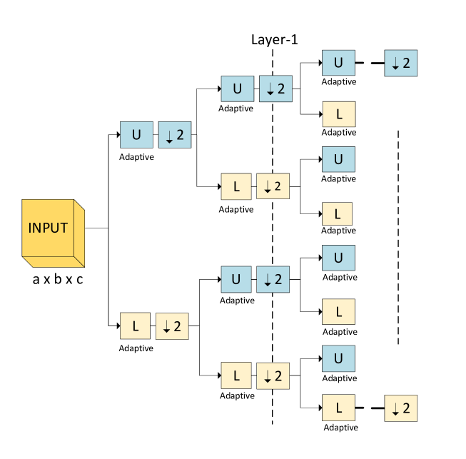
Fig. 1 depicts the ASD structure with layers. Similar to and in WSD [30], the and blocks represent decomposition filters. Specifically, each block comprises a collection of filters operating in parallel on the channels of the input. The filter for the th channel, , is a real 2-dimensional filter of order , where is an integer, with impulse response denoted by . Representing the input by a tensor of dimensions , , the output tensor is given by the convolution sum
| (1) |
The and blocks are followed by decimation-by-2 along the and dimensions only. Hence, at each layer, each channel of the input is split into four subbands with half the resolution along each of the and dimensions. This filtering-and-decimation process gets repeated for each subband as we move to the next decomposition layer. For example, for an input of size 224224 with 3 channels, i.e., 2242243, an a 1-layer subband decomposition provides four subbands with dimensions 1121123. For 2-layer decomposition, the same input yields 16 subbands of dimensions 56563 each. We note that the net dimension of the input and the final stack of the generated subbands are the same.
The network is end-to-end trained by back-propagating the error gradient up to the subband structures. It is, therefore, possible that, in contrast to WSD, the subbands may not be orthogonal leading to an overall lossless decomposition of the input signal. It is interesting to note that, as we show later, the subband structure learns filters of known types, such as band-pass, band-stop, low-pass, and high-pass structures, typically used in signal processing.
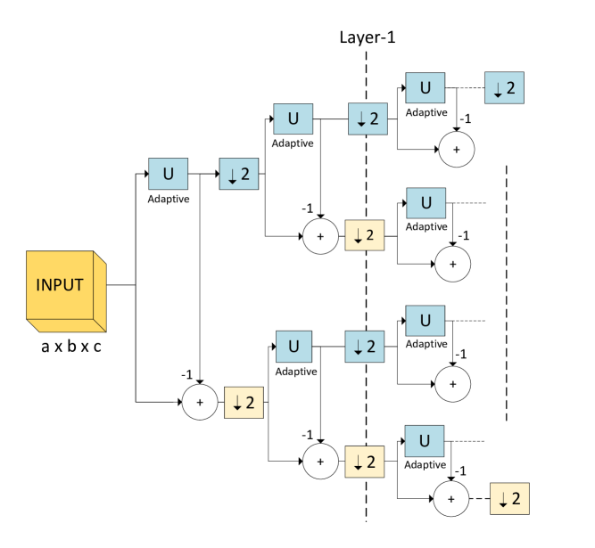
II-A2 Constrained Adaptive Subband Decomposition (CASD)
We can obtain a lossless subband decomposition that preserves the net information content of the input signal by further constraining the and filters into being spectrally complementary. The resulting CASD structure is shown in Fig. 2. As we can see, CASD is a special case of ASD with , i.e., has the same structure as in the case of ASD described in Section II-A1. The input-output relationship is given by (1) with . Similar to ASD, the network is end-to-end trained.
One of the benefits of the CASD structure is that it reduces the number of filter weights and, therefore, the computational cost of the subband decomposition structure at training by half; the cumulative effect of this reduction across training iterations can be significant. Another benefit of CASD is a higher degree of regularization compared to ASD which, depending on the dataset, can be beneficial. As we will see in the experimental results section, CASD (worse performance but also lower computational complexity) allows us to achieve a different tradeoff point than ASD which could be preferable depending on the application.
II-A3 Training of front-end structures
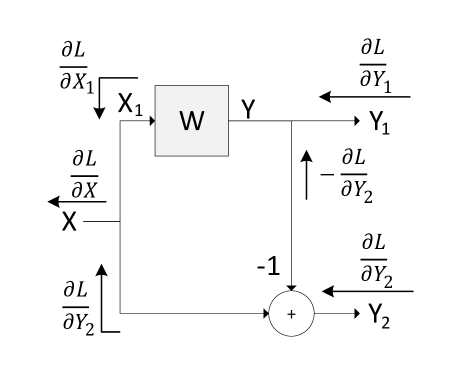
Note that the decomposition structures shown in Fig. 1 and Fig. 2 are regular convolution filter structures, and hence the standard back-propagation mechanism is applicable. We illustrate this by deriving the back-propagation equation for the CASD structure. Referring to Fig. 3, let be the loss function of the overall CNN, be the input, and and be the two outputs going to the next stage of the decomposition structure. Here and are complementary to each other in terms of spectral content [31], [32], ([c. 4, p. 125)]. Also, is the back-propagating error derivative wrt the output , , the error derivative wrt the weights , the error derivative wrt the input or the gradient passing down to the downstream module and the local gradient of the filter . Then, we can write
| (2) | ||||
| (3) | ||||
| (4) |
Computing is needed to propagate the error derivative while is required to update the filter weights.
II-B CNN Architectures
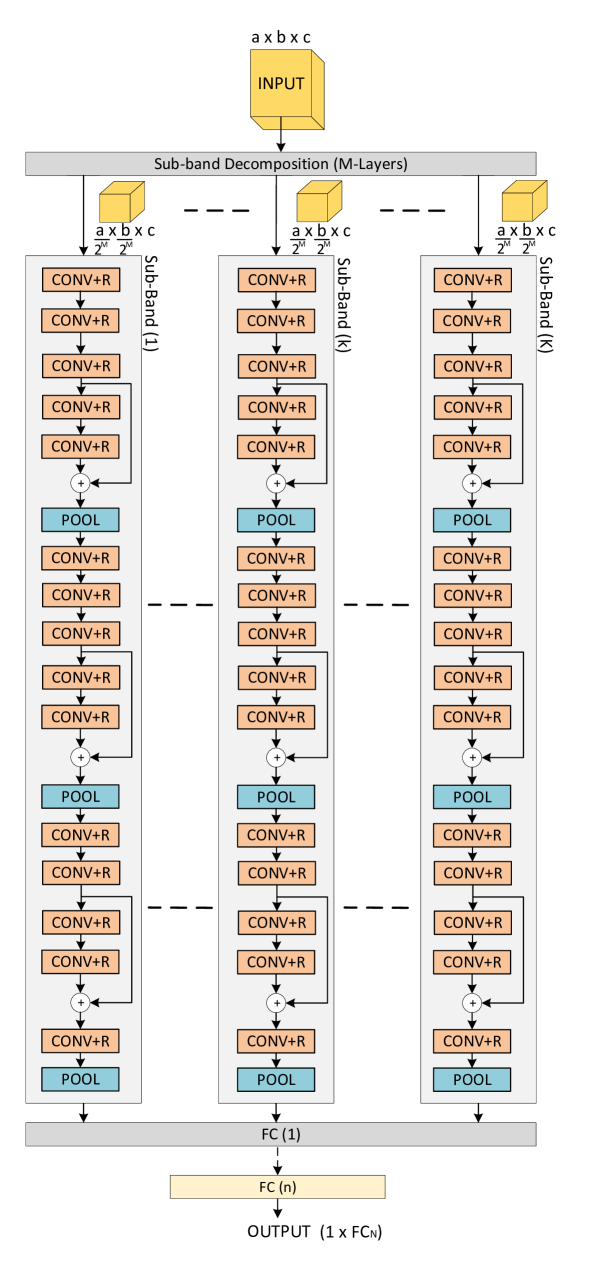
As described earlier, the subbands are processed by individual CNNs to extract relevant features before passing them through the fully connected (FC) layer for classification. The overall architecture called the MSR-CNN, is shown in Fig. 4. As a benchmark, we also consider a second architecture that passes the complete subband decomposition through a single CNN, as shown in Fig. 5(a). We call this architecture the SSR-CNN. Fig. 5(b) shows a second benchmark architecture, the Baseline CNN (BCNN). The BCNN architecture is similar to the MSR-CNN and the SSR-CNN in terms of the number of convolutional stages and the total FC layers, except the BCNN does not have the subband decomposition structure. Instead, the input image is passed directly into the CNN.
II-B1 Multi-Channel Subband Regularized CNN (MSR-CNN)
Fig. 4 shows the generalized -level MSR-CNN architecture in which the subbands are processed separately by individual CNNs, each with layers. This restricts the field of view of each CNN, making them indifferent to the rest of the subbands. The convolutional layers are similar to that of Alexnet [1] and/or VGG16 [7], with the difference of having a residual layer connection [9] before the pooling layer, as per Fig. 4. The addition of the residual layers, inspired by ResNet [9], significantly helps in speeding up training by allowing the error gradients to easily propagate to the initial layers. Finally, FC layers combine the feature outputs of the subband CNNs and perform classification.
We note that even though the input to the subband CNNs is already reduced in dimension, we still need pooling layers in the CNN to extract the dominant features per subband. This is done with a hierarchy of convolutional layers followed by a pooling layer that keeps the outputs with the largest magnitude, discarding the rest. In contrast, the decimation-by-2 blocks in the subband decomposition structure drop every 2nd filter output sample along the x and y dimensions, regardless of their magnitude. Therefore, the primary function of the wavelet subband decomposition is not to do dominant feature extraction. Rather, it assists in the extraction of the dominant features by the CNNs that follow.
II-B2 Single-Channel Subband Regularized CNN (SSR-CNN)
Fig. 5(a) shows the general architecture of SSR-CNN. The SSR-CNN architecture shares the same front-end subband decomposition structure as the MSR-CNN, i.e., ASD, CASD, or WSD. An -layer subband decomposition structure, with input tensor of dimensions , where , , and are the number of rows, columns, and channels, will result in total subbands, each represented by a tensor of dimensions . In contrast to the MSR-CNN architecture, all the channels of the subbands are stacked together and treated as a single input of dimension ) to a single CNN, followed by a fully connected layer to classify.
![[Uncaptioned image]](https://cdn.awesomepapers.org/papers/be455498-0eba-4759-a33b-8f6412805a8e/x6.png)
0.82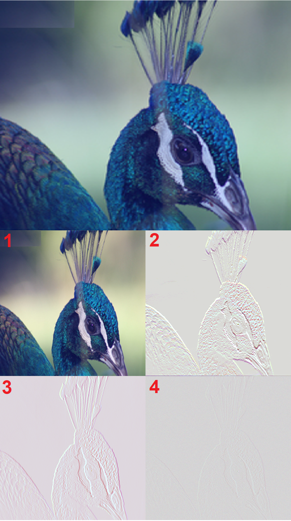
0.80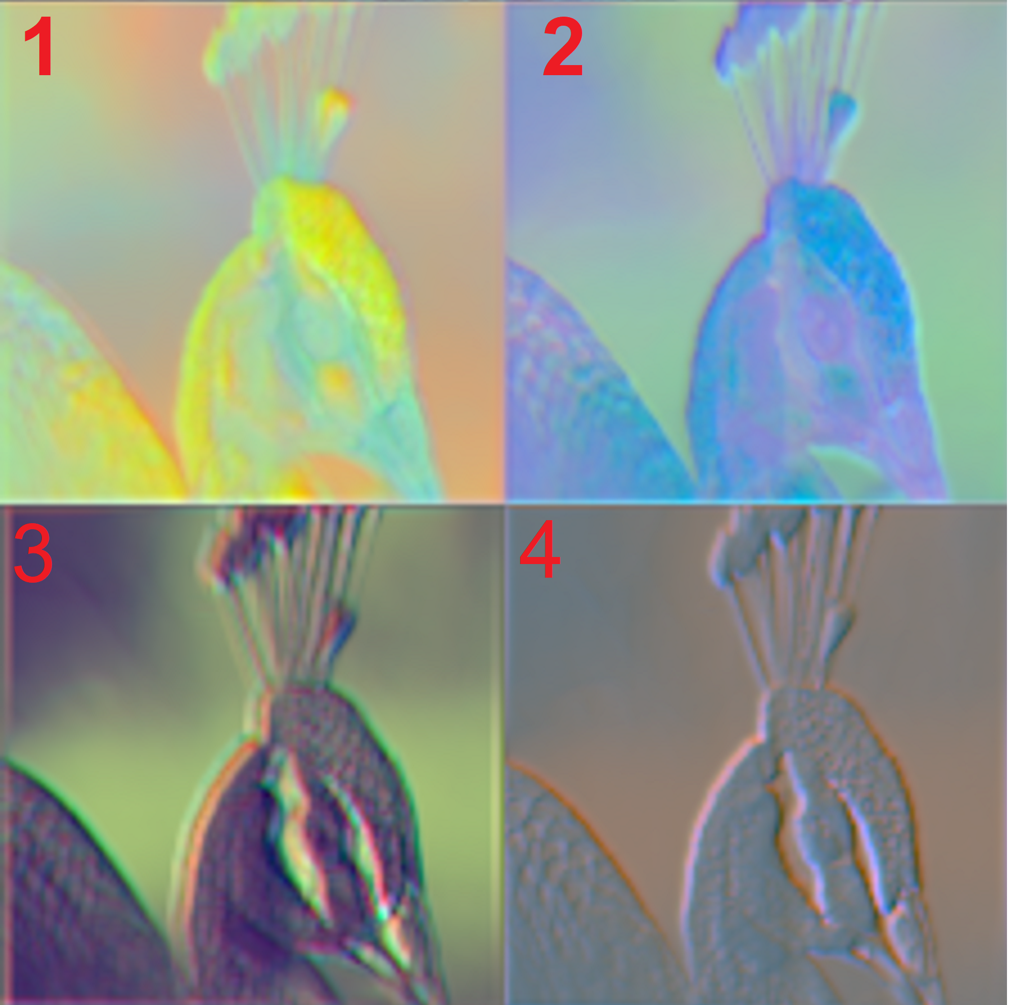
Both network architectures are end-to-end trained, meaning that the front-end structures (ASD or CASD), CNN and fully connected layers, are trained together by backpropagating the error derivative from the output layer all the way back to the front-end. As we will see, the ASD structure gives better accuracy over both CASD and WSD of [30], at the expense of higher computational cost. Furthermore, the CNN architecture with a CASD frontend performs better than with a WSD frontend, as shown in [30]. The WSD structure offers the least computation cost, while the CASD structure lies between the ASD and the WSD structures, balancing computation cost and performance.
III Properties of Proposed Architecture
In this section, we discuss several attractive properties of the proposed architecture. Specifically, we discuss the computational gains and the robustness towards quantization noise this architecture brings.
III-A Computational Cost
The proposed architecture offers a higher degree of parallelism as it allows for the independent processing of each subband. As we can see from Fig. 4, we have CNNs that operate in parallel compared to SSR-CNN or a single CNN in a traditional architecture (cf. Fig. 5(b)). Processing the individual subbands leads to a substantial reduction of the computational cost. The computational cost of all convolutional layers in a CNN with convolutions is [34], where is the number of filters at the th convolution ( is also referred to as the input depth of the th convolution), is the size of the convolution filter and the spatial size of the output of the th convolution.111It is assumed that the length and height of the convolution input are equal. If not, would be replaced by the product of the length and height of the input to the th convolution. Subband decomposition reduces the parameter by half along both length and height for every decomposition layer, significantly reducing the computational cost. The total reduction of input dimension along each subband is exponential and is given by for two-dimensional input data such as images. The reduction in computation complexity also applies to the back-propagation path. As we will see in the next section, the reduction in the total computation required for the forward pass and back-propagation over single-iteration is over 98% and 89%, respectively.
Sparsity in both weights and feature maps has motivated the development of different methods to take advantage of the available sparsity and optimize CNN computation requirements [35],[36], [37] and [38]. Typically, the information content of images is distributed unequally over the entire spectrum. Therefore, individual subbands generally exhibit higher sparsity compared to the entire spectrum. In the proposed subband decomposition structure, this sparsity is introduced at the very input of the subband CNNs. This makes it possible to use standard techniques that take advantage of sparsity to reduce CNN complexity, such as [39]. Finally, the proposed architectures can be combined with one of the numerous techniques to reduce the computational cost and memory requirements of CNNs. For example, by removing redundant kernels as in [40], or pruning of kernel coefficients [41]. The reader is referred to [42] for a detailed tutorial and survey of methods to reduce the CNN computational cost. We note, however, that exploring ways to further reduce the computational cost by applying on of the above techniques is beyond the scope of this work.
III-B Robustness to Input Noise and Quantization Errors
In practice, the input is subject to quantization noise and corruption due to non-linearities in the capturing device, e.g., lens aberration, incorrect exposure, low lighting condition, and a burst of transmission noise. Further, in most applications, signals are compressed before storage or transmission. For instance, image compression takes advantage of the unequal spread of information across the spectrum, allocating fewer bits to parts of the spectrum with less information [43],[44]. These sources of error ultimately result in noise that is spread unevenly across the spectrum. The subband decomposition of the input signal enables the network to analyze isolated subbands separately. This allows for noise within each subband to be confined within the subband. In contrast, in the case of a single full-spectrum input, any source of noise affects the entire spectrum.
A similar situation arises due to weight and bias quantization, which is imperative for practical implementation, where storage and computation in 64-bit floating-point representation become impossible. Several papers have studied weight quantization in CNNs, including [45], [46], and [47]. In CNNs that process the full spectrum of the signal, noise in each coefficient eventually affects the entire spectrum. In the proposed CNN architecture, however, weight and noise quantization noise is confined to individual subbands.
Our experimental studies show that the MSR-CNN is robust to input noise as well as weight and bias quantization noise. The ASD decomposition structure is shown to be the most robust compared to other subband decomposition structures. The CASD structure is the second most robust followed by the WSD structure in the third position. The superior performance of the ASD structure is owed to the ability of the ASD structure to learn from the dataset itself and the flexibility to adapt the subbands to reduce the loss during training without any constraints. The performance CASD is slightly lower than that of the ASD structure as a result of the complimentary subband decomposition structure and the restriction that comes along with it. The performance of the WSD structure indicates that within the constraints of our experimentation, fixed decomposition structures that cannot adapt to the dataset are sub-optimal in nature.
| Data-Set | MNIST and CIFAR-10/100 | Caltech-101 and ImageNet-2012 | ||||||||||
| Architecture | BCNN | SSR-CNN | MSR-CNN | BCNN | SSR-CNN | MSR-CNN | ||||||
| Input size | 28281 | 28281 | 28281 | 2242243 | 2242243 | 2242243 | ||||||
| Subbands | - | 1-Layer | 1-Layer | - | 1-Layer | 1-Layer | ||||||
| CONV | 33164 | 33464 | 331(64/4)4 | 33364 | 331264 | 333(64/4)4 | ||||||
| CONV | 3364128 | 3364128 |
|
336464 | 336464 | 33(64/4)(64/4)4 | ||||||
| CONV | 33128256 | 33128256 |
|
336464 | 336464 | 33(64/4)(64/4)4 | ||||||
| CONV | - | - | - | 336464 | 336464 | 33(64/4)(64/4)4 | ||||||
| CONV | - | - | - | 336464 | 336464 | 33(64/4)(64/4)4 | ||||||
| POOL | 2-by-2 | 2-by-2 | 2-by-2 | 2-by-2 | 2-by-2 | 2-by-2 | ||||||
| CONV | 33256512 | 33256 512 |
|
3364128 | 3364128 | 33(64/4) (128/4) 4 | ||||||
| CONV | 33512128 | 33512128 |
|
33128128 | 33128128 | 33(128/4) (128/4)4 | ||||||
| CONV | - | - | - | 33128128 | 33128128 | 33(128/4)(128/4)4 | ||||||
| CONV | - | - | - | 33128128 | 33128128 | 33(128/4)(128/4)4 | ||||||
| CONV | - | - | - | 33128128 | 33128128 | 33(128/4)(128/4)4 | ||||||
| POOL | 2-by-2 | - | N/A | 2-by-2 | 2-by-2 | 2-by-2 | ||||||
| CONV | - | - | - | 3364128 | 3364128 | 33(64/4) (128/4)4 | ||||||
| CONV | - | - | - | 33128128 | 33128128 | 33(128/4) (128/4)4 | ||||||
| CONV | - | - | - | 33128128 | 33128128 | 33(128/4) (128/4)4 | ||||||
| CONV | - | - | - | 33128128 | 33128128 | 33(128/4) (128/4)4 | ||||||
| CONV | - | - | - | 33128128 | 33128128 | 33(128/4) (128/4)4 | ||||||
| POOL | - | - | - | 2-by-2 | 2-by-2 | 2-by-2 | ||||||
| FC-1 | 77128 4096 | 77128 4096 | 771284096 |
|
|
|
||||||
| DROPOUT | 50% | 50% | 50% | 50% | 50% | 50% | ||||||
| FC-2 | 40961024 | 40961024 | 40961024 | 40964096 | 40961024 | 40961024 | ||||||
| DROPOUT | 50% | 50% | 50% | 50% | 50% | 50% | ||||||
| FC-3 | 102410 OR 1024101 | 102410 OR 1024101 | 102410 OR 1024101 | 4096101 OR 40961000 | 4096101 OR 40961000 | 4096101 OR 40961000 | ||||||
| SOFTMA | 110 OR 1101 | 110 OR 1101 | 110 OR 1101 | 1101 OR 11000 | 1101 OR 11000 | 1101 OR 11000 | ||||||
IV Experimental Setup and Results
In this section, we investigate the performance of the proposed methods on image classification problems. We note that the proposed methods can work on any two-dimensional input signal such as image, radar, Lidar, sonar, etc.
IV-A Data Sets
Our experiments use the MNIST, CIFAR-10/100, Caltech-101 and ImageNet-2012 datasets described in Table I. Images from both Caltech-101 and ImageNet-2012 datasets of varying sizes are resized to a common dimension of 2562563 using a Lanczos-3 kernel. The only pre-processing done is data augmentation, where we randomly pick patches of size 2242243 from the four corners and the center of the image. The overlap between the images reflects translation in the images from patch to patch, thereby preventing data repetition in the training set. Further, to prevent data repetition, we add Gaussian blur [53] with a filter kernel and standard deviation randomly picked between 0.5 and 1.5. We found that without this data augmentation, the model is heavily overfitting.
IV-B Models
We compare the proposed architecture against two benchmark models: the SSR-CNN described in Section II-B1, and the BCNN model shown in Fig. 5(b). The latter is a standard CNN that closely resembles AlexNet [1] and VGG-16 [7] and has ResNet-type [9] skip connections before each pooling layer. In contrast to BCNN, and similar to MSR-CNN, SSR-CNN also benefits from the exponential reduction of input data points per dimension, thereby substantially reducing the computational cost.
The parameters that determine the learning capacity of a CNN include the number of convolution layers, filters per layer, activation function, arrangement of pooling layers, and the number of FC layers. Table II shows the parameter values for the models, tuned heuristically due to the high computation cost of -fold cross-validation. To study the effect of learning in the subspace-based CNN architectures, we keep most parameters constant across BCNN, MSR-CNN, and SSR-CNN. A network with five convolutional, two pooling, and three FC layers are used for MNIST. A larger network of 15 convolutional, three pooling, and three FC layers are used for the CIFAR-10/100, Caltech-101, and ImageNet-2012 datasets. In all three models, each convolutional layer uses small receptive field filters of size pixels [7]. A max pooling is chosen for the pooling layers. We use 50% drop-out [1] at the first two FC layers to prevent significant overfitting, which helps reduce the difference in accuracy between training and test sets. We use no other regularization. Finally, at the last FC layer, we use Softmax.
For a fair comparison of MSR-CNN and SSR-CNN, we choose the total number of filters at each convolutional layer for both architectures to be equal, as seen in Table II. In addition, the number of FC layers and their parameters are kept the same for both architectures. The number of filters in each subband of the MSR-CNN is set to be equal to the total number of filters in the BCNN architecture divided by the number of subbands. For example, in a 1-layer decomposition structure, the number of filters in the first convolution layer of an MSR-CNN architecture, for each subband, is of the total number of filters in the first convolution layer of the BCNN architecture, i.e., if the first layer in BCNN has 64 filters, then MSR-CNN has 16 filters per subband, as shown in Table II. For comparison purposes, for the WSD structure, we chose the Daubechies (D2) family of basis functions for DWT [33].
IV-C Training
We train our models using stochastic gradient descent with a mini-batch size of 64, batch-normalized, randomly picked images per mini-batch, momentum set to 0.9, and weight decay set to 0.0005 as indicated in [1]. The update equations at the th iteration for the weights and biases of the convolutional filters at the th layer and th subband, , are given by:
| (5) |
where
| (6) |
Here is the momentum, the learning rate, and is the average over the th batch of the derivative of the objective function with respect to , evaluated at . The learning rate is initialized to 0.01 and later reduced by 10 when the validation error stops improving. We found experimentally that over a wide range of training sets, using a learning rate of 0.1, the networks showed minimal learning or did not learn at all, while with a learning rate of 0.001, learning was slow. It seems the best choice of learning rate lies between 0.1 and 0.001, so, we used a learning rate of 0.01 without optimizing this hyper-parameter further. The weight update equations given in equations (5) and (6) also govern the weight update of the subband decomposition filters. We use a lower learning rate for the subband decomposition structure compared to the subband convolutional layers because we have noticed that otherwise, the overall network is unable to learn effectively. We initialize the weights for both the subband structure and the CNN weights by drawing from a Gaussian distribution with a standard deviation of 0.01. All biases are initialized to 1.
The following four parallel threads are run in the pipeline: (i) Read mini-batch from storage disk and re-size images, (ii) Compute data augmentation, (iii) Compute decomposition filters (2D-DWT/ASD/CASD) on CPU, and (iv) Transfer data to GPU, compute CNN on GPU, and read-back to system main memory. The GPU computation is the bottleneck, thereby resulting in almost free processing time for the rest of the parallel threads per batch. Pipeline fill-&-flush are processed accordingly, with pipeline overhead being insignificant compared to total processing time.
During testing, while reading in the input image, we pick five patches from the input image, four from the four corners, and one from the center. Predictions on these five patches are then averaged to obtain the final result of that single input image. Finally, we average over the entire test dataset to get the final test result.
IV-D Results
IV-D1 Qualitative analysis of subband decomposition
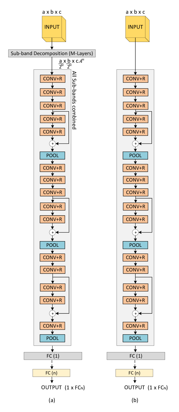
In Fig. 6, we show examples of the 2D frequency responses of the first layer of the ASD filter structure (cf. Fig. 1). The top row shows the 2D frequency response of the filters in the first upper and lower paths that decompose the input signal into two subbands. The bottom row shows the 2D frequency response of the filters in the second set of upper and lower paths that completes the first layer decomposing the input into four subbands. Note that the first-row filter responses are low-pass (left) and high-pass (right), while the second row of filters consists of low-pass, wider range low-pass, band-pass, and high-pass filter frequency responses, from left to right, respectively. Interestingly, the learned filters in the proposed structure resemble subband decomposition filters, i.e., pairs of highpass and lowpass filters, typically used in signal processing.
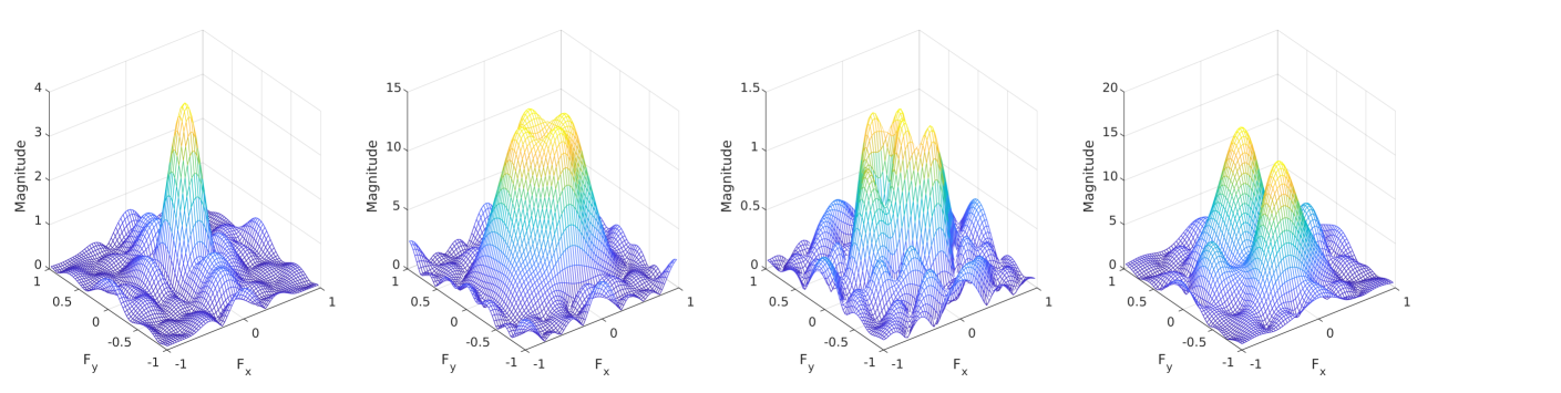
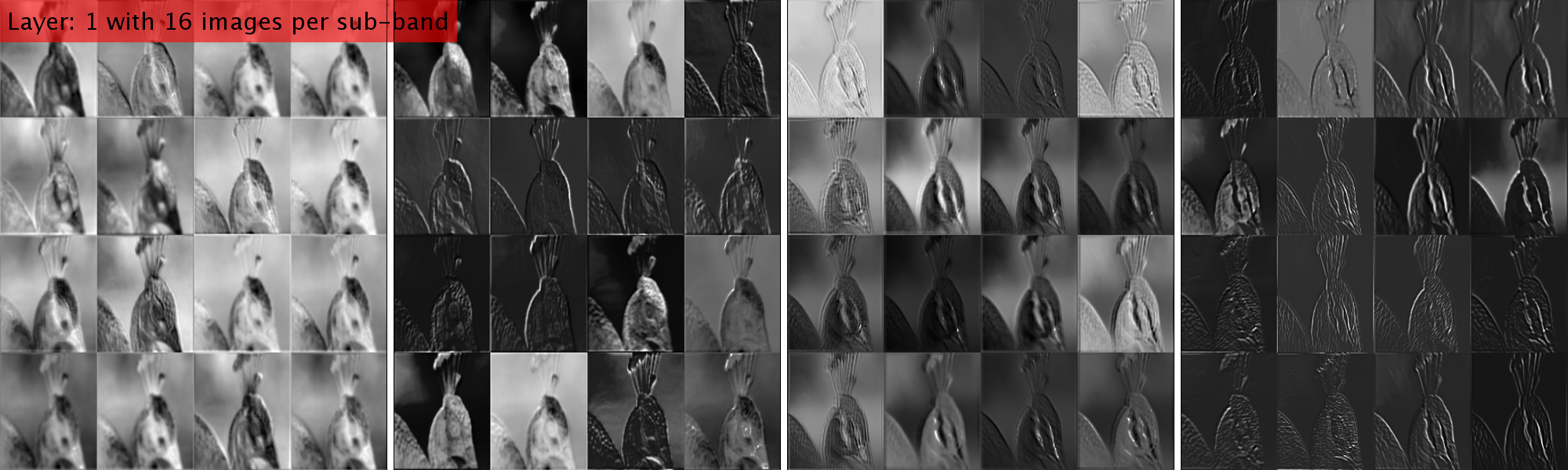
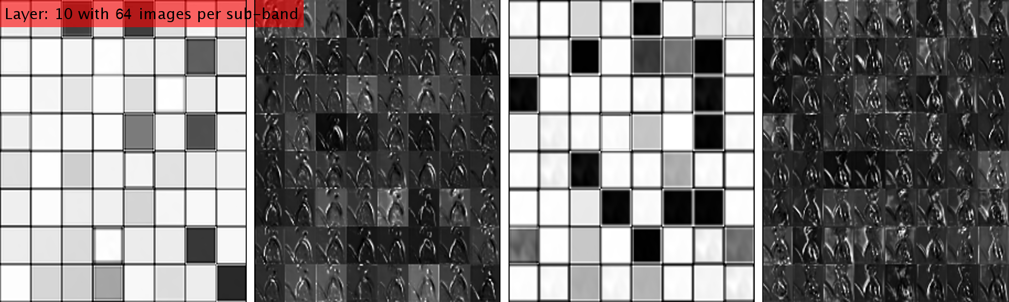
Fig. 7 shows the input image and the 4 subbands of a 1-layer 2D-DWT decomposition filter structure while Fig. 8 shows the 4 subbands of a 1-layer ASD decomposition filter structure in MSR-CNN for the same input image. Fig. 9 shows the output of the first convolutional layer of MSR-CNN with a 1-layer ASD structure. Though all subbands have a mix of low and high-frequency components, the subbands to the left have more low-frequency components while the subbands to the right have more high-frequency components as seen in the activation map. Fig. 10 shows the output at the 10th convolutional layer. In contrast to Fig. 9, Fig. 10 has lost the details in LL and UL subbands containing mainly low frequency or DC components, while the other two subbands still resemble the input and highlight specific contours of the input, indicating high-frequency components. The FC layer utilizes this collective information to partition the output hyperspace.
IV-D2 Classification Accuracy
In Table III we present the top-1 accuracy comparison across the BCNN, SSR-CNN, and MSR-CNN architectures, for both 1- and 2-layer ASD and CASD structures. We have used a filter of order five for both the ASD and CASD filter structures. Generally, we notice a drop in performance going to a 2-layer decomposition compared to a 1-layer decomposition structure. This drop is a tradeoff between performance and computation cost. We also observe that the ASD structure with the MSR-CNN performs the best across different datasets.
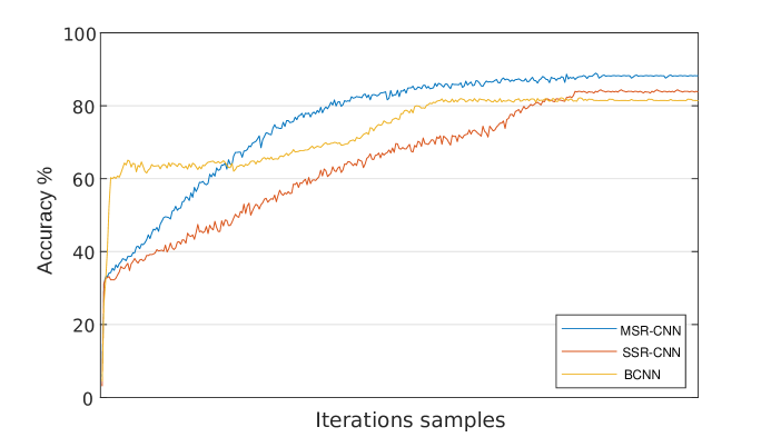
Fig. 11 compares the test-set error curves of the BCNN, SSR-CNN, and MSR-CNN architectures. Compared to both the BCNN and the SSR-CNN curves, we find that the accuracy of the MSR-CNN has a milder monotonically increasing trajectory before settling down to a higher accuracy value. The BCNN increases quickly, then remains relatively stable, and finally shows an increase in accuracy before settling to a lower value compared to MSR-CNN and the SSR-CNN. The SSR-CNN on the other hand makes an initial jump in accuracy like that of the MSR-CNN and thereafter improves in accuracy in an almost linear fashion until settling between the performance of the MSR-CNN and the BCNN. This indicates that, with a 1-layer ASD structure, the better regularization of the MSR-CNN architecture results in more effective training compared to the BCNN and the SSR-CNN architectures.
On the ImageNet-2012 dataset, the MSR-CNN architecture with 1-layer ASD structure achieves top-5 and top-1 validation set accuracy of 86.91% and 69.45%, respectively. Unlike most popular networks, we did not perform architectural hyper-parameter optimization due to the lack of heavy computational resources, leaving room for further improvements.
| Model | Decomposition | Dataset | Accuracy % (Top-1) |
| BCNN | - | Caltech-101 | 82.17 |
| SSR-CNN | 1-layer (WSD) | Caltech-101 | 83.89 |
| SSR-CNN | 1-layer (CASD) | Caltech-101 | 87.47 |
| SSR-CNN | 1-layer (ASD) | Caltech-101 | 89.05 |
| MSR-CNN | 1-layer (WSD) | Caltech-101 | 87.79 |
| MSR-CNN | 1-layer (CASD) | Caltech-101 | 88.13 |
| MSR-CNN | 1-layer (ASD) | Caltech-101 | 89.39 |
| SSR-CNN | 2-layer (CASD) | Caltech-101 | 79.67 |
| SSR-CNN | 2-layer (ASD) | Caltech-101 | 79.39 |
| MSR-CNN | 2-layer (CASD) | Caltech-101 | 80.94 |
| MSR-CNN | 2-layer (ASD) | Caltech-101 | 82.49 |
| BCNN | - | ImageNet-2012 | 63.21 |
| SSR-CNN | 1-layer (CASD) | ImageNet-2012 | 65.95 |
| SSR-CNN | 1-layer (ASD) | ImageNet-2012 | 66.84 |
| MSR-CNN | 1-layer (CASD) | ImageNet-2012 | 67.98 |
| MSR-CNN | 1-layer (ASD) | ImageNet-2012 | 69.45 |
| SSR-CNN | 2-layer (CASD) | ImageNet-2012 | 59.25 |
| SSR-CNN | 2-layer (ASD) | ImageNet-2012 | 59.67 |
| MSR-CNN | 2-layer (CASD) | ImageNet-2012 | 61.87 |
| MSR-CNN | 2-layer (ASD) | ImageNet-2012 | 62.73 |
| BCNN | - | MNIST | 99.72 |
| SSR-CNN | 1-layer (WSD) | MNIST | 99.76 |
| SSR-CNN | 1-layer (CASD) | MNIST | 99.79 |
| SSR-CNN | 1-layer (ASD) | MNIST | 99.83 |
| MSR-CNN | 1-layer (WSD) | MNIST | 99.81 |
| MSR-CNN | 1-layer (CASD) | MNIST | 99.83 |
| MSR-CNN | 1-layer (ASD) | MNIST | 99.89 |
| BCNN | - | CIFAR-10 | 95.37 |
| SSR-CNN | 1-layer (WSD) | CIFAR-10 | 96.59 |
| SSR-CNN | 1-layer (CASD) | CIFAR-10 | 97.79 |
| SSR-CNN | 1-layer (ASD) | CIFAR-10 | 97.81 |
| MSR-CNN | 1-layer (WSD) | CIFAR-10 | 96.71 |
| MSR-CNN | 1-layer (CASD) | CIFAR-10 | 96.82 |
| MSR-CNN | 1-layer (ASD) | CIFAR-10 | 97.86 |
| BCNN | - | CIFAR-100 | 80.72 |
| SSR-CNN | 1-layer (WSD) | CIFAR-100 | 81.83 |
| SSR-CNN | 1-layer (CASD) | CIFAR-100 | 81.74 |
| SSR-CNN | 1-layer (ASD) | CIFAR-100 | 82.95 |
| MSR-CNN | 1-layer (WSD) | CIFAR-100 | 82.97 |
| MSR-CNN | 1-layer (CASD) | CIFAR-100 | 83.75 |
| MSR-CNN | 1-layer (ASD) | CIFAR-100 | 85.07 |
IV-D3 Computational Cost
In Table IV, we compare the total computation cost for both inference and training operations, of MSR-CNN and SSR-CNN architectures with the ASD structure. The reported numbers take into account every addition and multiplication operation performed by each network. The total addition and multiplication operations involved in the convolution operations dominate the overall computational cost of the CNNs. In the case of the back-propagation path, we take into account the number of operations per iteration. In the case of the inference path, which is not iterative, we report the total number of operations. With a 1-layer ASD structure, the MSR-CNN achieves nearly two orders of magnitude reduction in total addition and multiplication operations relative to the BCNN. The total number of addition and multiplication operations reduces further going to a 2-layer subband decomposition structure. When integrated over the period of training, it significantly reduces the total operations or the total energy spent. The above significant computational cost reductions are directly attributed to the number of filters in each architecture. We note that the number of filters in the ASD filter is filters, where is the number of layers. In comparison, the CASD filter structure requires filters. For example, a 3-layer ASD structure would have 126 such filters to compute, while the 3-layer CASD structure would only have 63 such filters to compute.
| Inference | Total Reduction (%) w.r.t BCNN | |
|---|---|---|
| Additions | Multiplications | |
| SSR-CNN (1L) | 77.64 | 76.11 |
| MSR-CNN (1L) | 95.75 | 95.47 |
| SSR-CNN (2L) | 95.52 | 95.22 |
| MSR-CNN (2L) | 98.84 | 98.76 |
| Training | Total Reduction (%) w.r.t BCNN | |
| Additions | Multiplications | |
| SSR-CNN (1L) | 72.84 | 72.50 |
| MSR-CNN (1L) | 75.93 | 74.47 |
| SSR-CNN (2L) | 81.11 | 90.28 |
| MSR-CNN (2L) | 89.07 | 94.13 |
| Models |
|
MACs |
|
|
|
|
|
||||||||||||
|---|---|---|---|---|---|---|---|---|---|---|---|---|---|---|---|---|---|---|---|
| MobileNet V1 [54] | 12.44 | 569 (M) | 4.24 | 2 | 70.9 | 89.9 | 19 | ||||||||||||
| MobileNet V2 [55] | 14.63 | 300 (M) | 3.47 | 1.7 | 71.8 | 91 | 19.2 | ||||||||||||
| Google Net [8] | 9.22 | 741 (M) | 6.99 | 3.3 | - | 92.1 | - | ||||||||||||
| AlexNet [1] | 1.49 | 724 (M) | 60.95 | 29.1 | 62.5 | 83 | 20.5 | ||||||||||||
| SqueezeNet [14] | 8.48 | 833 (M) | 1.24 | 0.6 | 57.5 | 80.3 | 22.8 | ||||||||||||
| ResNet-50 [9] | 6.47 | 3.9 (B) | 25.6 | 12.2 | 75.2 | 93 | 17.8 | ||||||||||||
| VGG [7] | 9.21 | 15.5 (B) | 138 | 65.8 | 70.5 | 91.2 | 20.7 | ||||||||||||
| Inception-V1 [11] | 2.45 | 1.43 (B) | 7 | 3.3 | 69.8 | 89.3 | 19.5 | ||||||||||||
| MSR-CNN (1L) | 1.52 | 169.5 (M) | 42.05 | 20.1 | 69.45 | 86.91 | 15.68 | ||||||||||||
| MSR-CNN (2L) | 0.79 | 46.34 (M) | 13.64 | 6.5 | 62.73 | 79.15 | 16.42 |
| Datasets | Models | 1-bit | 2-bits | 4-bits | 6-bits | 8-bits |
| MNIST | BCNN | 97.42 | 97.53 | 97.6 | 97.69 | 99.72 |
| SSR-CNN (WSD) | 97.87 | 98.03 | 99.45 | 99.53 | 99.76 | |
| SSR-CNN (CASD) | 96.23 | 98.03 | 99.47 | 99.58 | 99.79 | |
| SSR-CNN (ASD) | 97.23 | 98.57 | 99.57 | 99.61 | 99.83 | |
| MSR-CNN (WSD) | 99.5 | 99.6 | 99.63 | 99.64 | 99.81 | |
| MSR-CNN (CASD) | 96.75 | 99.65 | 99.69 | 99.72 | 99.83 | |
| MSR-CNN (ASD) | 99.5 | 99.69 | 99.71 | 99.76 | 99.89 | |
| CIFAR-10 | BCNN | 76.36 | 76.06 | 76.39 | 85.66 | 95.37 |
| SSR-CNN (WSD) | 76.66 | 76.38 | 79.2 | 89.56 | 96.59 | |
| SSR-CNN (CASD) | 76.67 | 76.38 | 79.38 | 90.45 | 97.79 | |
| SSR-CNN (ASD) | 76.66 | 76.38 | 87.45 | 93.49 | 97.81 | |
| MSR-CNN (WSD) | 78.13 | 79.2 | 80.03 | 91.32 | 96.71 | |
| MSR-CNN (CASD) | 79.04 | 80.56 | 84.76 | 92.25 | 96.82 | |
| MSR-CNN (ASD) | 78.13 | 82.38 | 87.03 | 95.39 | 97.86 | |
| CIFAR-100 | BCNN | 54.89 | 59.66 | 68.8 | 73.85 | 80.72 |
| SSR-CNN (WSD) | 58.91 | 61.03 | 69.87 | 74.75 | 81.74 | |
| SSR-CNN (CASD) | 59.79 | 63.78 | 70.98 | 76.76 | 82.83 | |
| SSR-CNN (ASD) | 58.91 | 66.03 | 74.87 | 79.75 | 84.74 | |
| MSR-CNN (WSD) | 60.14 | 64.79 | 69.15 | 74.07 | 82.97 | |
| MSR-CNN (CASD) | 61.23 | 65.45 | 70.56 | 76.87 | 83.75 | |
| MSR-CNN (ASD) | 60.14 | 66.79 | 72.15 | 77.07 | 85.07 | |
| CALTECH-101 | BCNN | 69.87 | 71.96 | 76.2 | 79.31 | 82.17 |
| SSR-CNN (WSD) | 71.66 | 76.29 | 80.91 | 81.47 | 83.89 | |
| SSR-CNN (CASD) | 69.89 | 76.14 | 81.04 | 82.67 | 84.07 | |
| SSR-CNN (ASD) | 71.66 | 77.02 | 82.31 | 84.01 | 85.95 | |
| MSR-CNN (WSD) | 71.17 | 74.94 | 77.61 | 83.16 | 86.93 | |
| MSR-CNN (CASD) | 71.48 | 75.47 | 79.89 | 84.67 | 88.13 | |
| MSR-CNN (ASD) | 72.17 | 75.94 | 79.94 | 84.74 | 89.39 |
| Datasets | Models | 8-bits | 16-bits | 32-bits |
| MNIST | BCNN | 90.3 | 97.53 | 99.72 |
| SSR-CNN (WSD) | 90.91 | 97.9 | 99.76 | |
| SSR-CNN (CASD) | 90.95 | 98.56 | 99.79 | |
| SSR-CNN (ASD) | 90.91 | 99.01 | 99.83 | |
| MSR-CNN (WSD) | 91.65 | 99.65 | 99.81 | |
| MSR-CNN (CASD) | 91.95 | 99.66 | 99.83 | |
| MSR-CNN (ASD) | 93.95 | 99.75 | 99.89 | |
| CIFAR-10 | BCNN | 60.85 | 76.13 | 95.37 |
| SSR-CNN (WSD) | 61.37 | 79.46 | 96.59 | |
| SSR-CNN (CASD) | 63.45 | 81.94 | 97.79 | |
| SSR-CNN (ASD) | 65.37 | 83.46 | 97.81 | |
| MSR-CNN (WSD) | 63.54 | 79.84 | 96.71 | |
| MSR-CNN (CASD) | 64.45 | 81.34 | 96.82 | |
| MSR-CNN (ASD) | 63.54 | 79.84 | 97.86 | |
| CIFAR-100 | BCNN | 61.17 | 73.78 | 80.72 |
| SSR-CNN (WSD) | 61.13 | 61.13 | 81.83 | |
| SSR-CNN (CASD) | 59.56 | 70.45 | 81.74 | |
| SSR-CNN (ASD) | 61.13 | 71.13 | 82.95 | |
| MSR-CNN (WSD) | 63.15 | 61.37 | 82.97 | |
| MSR-CNN (CASD) | 61.65 | 70.02 | 83.75 | |
| MSR-CNN (ASD) | 63.15 | 71.37 | 85.07 | |
| CALTECH-101 | BCNN | 59.13 | 79.67 | 82.17 |
| SSR-CNN (WSD) | 75.4 | 80.01 | 83.89 | |
| SSR-CNN (CASD) | 80.23 | 81.23 | 87.47 | |
| SSR-CNN (ASD) | 75.4 | 80.01 | 89.05 | |
| MSR-CNN (WSD) | 82.35 | 83.16 | 87.79 | |
| MSR-CNN (CASD) | 81.23 | 84.23 | 88.13 | |
| MSR-CNN (ASD) | 82.35 | 83.16 | 89.39 |
IV-D4 Comparisons to state-of-the-art
In Table V we present a comprehensive comparison of well-established CNN architectures [54],[55],[8],[1],[14],[9],[7], and [11] against the best performer among the proposed CNN architectures. The comparison is in terms of time taken, number of multiply-and-accumulate (MAC) units, number of total parameters, and CNN performance accuracy percentage for the ImageNet-2012 dataset. The computation time was evaluated on a DELL PowerEdge R740xd server with 256 GB DDR4 2666MT/S, dual Intel-Xeon Gold 5220 CPUs with 18 cores each, and an Nvidia GTX 1080Ti GPU with Nvidia CUDA and cuDNN libraries. The results were obtained using 1000 images with a batch size of 8 images for all models. As we can see, the MSR-CNN with the 1-layer ASD structure performs the best, with an accuracy of 86.91% with 169.5M MAC operations and 42.05M parameters, which takes around 1.52 seconds to process 1000 images with a batch size of 8 images.
Both the 1-layer and 2-layer subband decomposed MSR-CNNs give a best-in-class reduction in total MAC operations needed. The MSR-CNN with 1-layer decomposition takes 169.5M MAC operations while the 2-layer decomposition takes 46.34M MAC operations. Other models range between 300M to 15.5B MAC operations. On the number of parameters front, the MSR-CNN architecture performs fairly. The parameters of all compared CNNs require between 0.6 to 65.8 MBytes, with the 1-layer and 2-layer MSR-CNN architectures at 20.1 and 6.5 MBytes, respectively. In practice, the difference between 6.5 and 0.6 MBytes can be ignored, whereas a 10 reduction in total MAC operations can significantly improve computation time. Finally, based on our experimental setup, the 1-layer, and 2-layer MSR-CNN take 1.52 secs and 0.79 sec respectively, while the other models range between 1.49 secs and 14.63 secs.
IV-D5 Quantization Effect
In Table VI, we show the effect of different levels of input quantization for the BCNN, SSR-CNN, and MSR-CNN architectures with WSD, 1-layer CASD, and 1-layer ASD. We quantize the input at 1, 2, 4, 6, and 8 bits. All internal computations are performed using the IEEE 32-bit floating-point precision. The objective of this experiment is to analyze the effect of input quantization noise on CNN accuracy results over various CNN architectures, subband decomposition structures, quantization levels, and datasets. We clearly observe that all three subband decomposition structures, WSD, CASD, and ASD are highly robust towards input quantization noise compared to the full-band BCNN architecture. The results in Table VI indicate that: 1) The subband decomposition structures provide robustness to input quantization error compared to full-band CNN architecture. 2) The effect of input quantization on the subband decomposition architectures is not drastic, even when we go down to 1-bit quantization. This is not so surprising since even a human can fairly recognize an image well with 1-bit quantization. For instance, grayscale newspaper printing used 1-bit greyscale with dithering [56]. Further, screens often use only 4-to-5 bits of color per channel natively and yet display good quality images, thanks to dithering [57]. Dithering fundamentally manipulates quantization noise by reshaping and spreading the noise unevenly across the spectrum. The subband decomposition process offers better input quantization even at 1-bit, compared to BCNN. 3) For applications requiring low transmission data rates or low storage and that intend to save power and computation resources, the flexibility offered by MSR-CNN with an adaptive subband decomposition front-end to quantize the input images to a greater extent without significantly affecting performance is advantageous from a system design consideration.
Weight-and-bias quantization plays a very important role in the implementation of CNNs in real-life systems [58]. Without weight and bias quantization, it would have been impractical to implement a CNN in an embedded system, where storage space and computation resources are limited. The ability to quantize at 8 bits compared to a 32-bit and 64-bit implementation is a matter of and savings in direct storage space, respectively. Quantization of weight and bias also results in a lower memory footprint during the computation of the CNN model. In Table VII, we investigate the effect of weight and bias quantization noise on inference accuracy for the BCNN, SSR-CNN, and MSR-CNN architectures with 1-layer WSD, CASD, and ASD for four different datasets, MNIST, CIFAR-10/100, and Caltech-101. In this experiment, we consider different quantization levels such as 8-bit, 16-bit, and 32 bits. All internal computations are performed using the IEEE 32-bit floating-point precision. Results from Table VII indicate that: 1) The subband decomposition structure provides robustness to weight and bias quantization error compared to full-band CNN architecture. 2) The MSR-CNN with the ASD subband decomposition structure, in general, performs better than the other architectures. 3) The ability of MSR-CNN with an adaptive subband decomposition front-end to perform better with heavily quantized weights and biases makes it an attractive choice for applications that are highly sensitive to computation and storage resources.
Both Tables VI and VII indicate that the MSR-CNN with the ASD decomposition structure performs the best. For applications with an additional need for reducing computation resources, the CASD structure may be a suitable compromise between computation cost and performance. As a final note, we would like to emphasize that the proposed architectures can be combined with sophisticated weight quantization methods, e.g., range batch normalization. Investigation of which method complements better the proposed architectures is beyond the scope of this work.
V Conclusion
We proposed two novel structures for learning the input signal decomposition into subbands: the ASD and the CASD structures. We incorporated these structures into a CNN architecture where each subband is individually processed via a separate CNN. The proposed structures integrate well with the end-to-end learning mechanism of a CNN. In the context of neural network-based image classification, we showed that the proposed CNN architecture achieves robust and near state-of-the-art performance compared to analyzing the entire spatial representation by a single CNN. Importantly, this performance comes at less than of the computation cost of an equivalent full-band CNN. Three main factors contribute to such performance: First, structural regularization is inherent to the proposed architecture. Second, a given subband is protected from noise and other deformities, e.g., input quantization error and weight-and-bias quantization error, present in the rest of the subbands. Third, the reduction of input dimensions of the convolution operation at each layer reduces the computational cost. Ultimately, we would like to apply the efficient architecture to video sequence prediction, where computation cost grows exponentially due to the added dimension of time.
References
- [1] A. Krizhevsky, I. Sutskever, and G. E. Hinton, “Imagenet classification with deep convolutional neural networks,” in Advances in Neural Information Processing Systems, 2012, pp. 1097–1105.
- [2] J. Long, E. Shelhamer, and T. Darrell, “Fully convolutional networks for semantic segmentation,” 2015.[Online]. Available: arXiv:1411.4038.
- [3] O. Vinyals, A. Toshev, S. Bengio, and D. Erhan, “Show and tell: A neural image caption generator,” 2015.[Online]. Available: arXiv:1411.4555.
- [4] A. Toshev and C. Szegedy, “DeepPose: Human pose estimation via deep neural networks,” in 2014 IEEE Conference on Computer Vision and Pattern Recognition. IEEE, jun 2014. [Online]. Available: https://doi.org/10.1109%2Fcvpr.2014.214
- [5] Y. Lecun, L. Bottou, Y. Bengio, and P. Haffner, “Gradient-based learning applied to document recognition,” in Proceedings of the IEEE, 1998, pp. 2278–2324.
- [6] M. D. Zeiler and R. Fergus, “Visualizing and understanding convolutional networks,” 2013.[Online]. Available: arXiv:1311.2901.
- [7] K. Simonyan and A. Zisserman, “Very deep convolutional networks for large-scale image recognition,” 2015.[Online]. Available: arXiv:1409.1556.
- [8] C. Szegedy, W. Liu, Y. Jia, P. Sermanet, S. Reed, D. Anguelov, D. Erhan, V. Vanhoucke, and A. Rabinovich, “Going deeper with convolutions,” 2014.[Online]. Available: arXiv:1409.4842.
- [9] K. He, X. Zhang, S. Ren, and J. Sun, “Deep residual learning for image recognition,” 2015.[Online]. Available: arXiv:1512.03385.
- [10] M. Jaderberg, K. Simonyan, A. Zisserman, and K. Kavukcuoglu, “Spatial transformer networks,” 2016.[Online]. Available: arXiv:1506.02025.
- [11] C. Szegedy, W. Liu, Y. Jia, P. Sermanet, S. E. Reed, D. Anguelov, D. Erhan, V. Vanhoucke, and A. Rabinovich, “Going deeper with convolutions,” in IEEE Conf. Computer Vision and Pattern Recog., CVPR, 2015, pp. 1–9.
- [12] K. He, X. Zhang, S. Ren, and J. Sun, “Spatial pyramid pooling in deep convolutional networks for visual recognition,” IEEE Trans. Pattern Anal. Mach. Intell., vol. 37, no. 9, pp. 1904–1916, 2015.
- [13] G. Koch, R. Zemel, and R. Salakhutdinov, “Siamese neural networks for one-shot image recognition,” in 32nd International Conference on Machine Learning, 2015.
- [14] F. N. Iandola, S. Han, M. W. Moskewicz, K. Ashraf, W. J. Dally, and K. Keutzer, “Squeezenet: Alexnet-level accuracy with 50x fewer parameters and <0.5mb model size,” 2016.[Online]. Available: arXiv:1602.07360.
- [15] O. M. Parkhi, A. Vedaldi, and A. Zisserman, “Deep face recognition,” in BMVC, 2015.
- [16] Q. Cao, L. Shen, W. Xie, O. M. Parkhi, and A. Zisserman, “Vggface2: A dataset for recognising faces across pose and age,” 2018.[Online]. Available: arXiv:1710.08092.
- [17] F. Schroff, D. Kalenichenko, and J. Philbin, “FaceNet: A unified embedding for face recognition and clustering,” in 2015 IEEE Conference on Computer Vision and Pattern Recognition (CVPR). IEEE, jun 2015.
- [18] Y. Liu, Y.-H. Wu, G. Sun, L. Zhang, A. Chhatkuli, and L. V. Gool, “Vision transformers with hierarchical attention,” 2022.[Online]. Available: arXiv:2106.03180.
- [19] K. Crammer, A. Kulesza, and M. Dredze, “Adaptive regularization of weight vectors,” in Advances in Neural Information Processing Systems 22. Curran Associates, Inc., 2009, pp. 414–422.
- [20] X. Sun, “Structure regularization for structured prediction: Theories and experiments,” 2015.[Online]. Available: arXiv:1411.6243.
- [21] A. Tong, D. van Dijk, J. S. Stanley, III, M. Amodio, G. Wolf, and S. Krishnaswamy, “Graph Spectral Regularization for Neural Network Interpretability,” ArXiv e-prints, Sep. 2018.
- [22] V. N. Ekambaram, G. Fanti, B. Ayazifar, and K. Ramchandran, “Wavelet-regularized graph semi-supervised learning,” in 2013 IEEE Global Conference on Signal and Information Processing, Dec 2013, pp. 423–426.
- [23] S.-C. B. Lo, H. Li, J.-S. Lin, A. Hasegawa, C. Y. Wu, M. T. Freedman, and S. K. Mun, “Artificial convolution neural network with wavelet kernels for disease pattern recognition,” Proc.SPIE, vol. 2434, pp. 1 – 10, 1995.
- [24] E. Kang, J. Min, and J. C. Ye, “A deep convolutional neural network using directional wavelets for low-dose x-ray CT reconstruction,” Medical Physics, vol. 44, no. 10, pp. e360–e375, oct 2017.
- [25] T. Williams and R. Li, “Advanced image classification using wavelets and convolutional neural networks,” in 2016 15th IEEE International Conference on Machine Learning and Applications (ICMLA), 2016, pp. 233–239.
- [26] S. Fujieda, K. Takayama, and T. Hachisuka, “Wavelet convolutional neural networks,” 2018.[Online]. Available: arXiv:1805.08620.
- [27] M. Ulicny, V. A. Krylov, and R. Dahyot, “Harmonic convolutional networks based on discrete cosine transform,” 2022.[Online]. Available: arXiv:2001.06570.
- [28] E. Oyallon, E. Belilovsky, S. Zagoruyko, and M. Valko, “Compressing the input for CNNs with the first-order scattering transform,” in Computer Vision – ECCV 2018. Springer International Publishing, 2018, pp. 305–320.
- [29] J. Bruna and S. Mallat, “Invariant scattering convolution networks,” 2012.[Online]. Available: arXiv:1203.1513.
- [30] P. Sinha, I. Psaromiligkos, and Z. Zilic, “A structurally regularized convolutional neural network for image classification using wavelet-based subband decomposition,” in 2019 IEEE International Conference on Image Processing (ICIP), 2019, pp. 649–653.
- [31] L. Wanhammar, DSP Integrated Circuits. Elsevier, 1999.
- [32] L. D. Milić and J. D. ćertić, “Recursive digital filters and two-channel filter banks: Frequency-response masking approach,” in 2009 9th International Conference on Telecommunication in Modern Satellite, Cable, and Broadcasting Services, 2009, pp. 177–184.
- [33] D. I, “The wavelet transform, time-frequency localization and signal analysis,” IEEE Transactions on Information Theory, vol. 36, no. 5, pp. 961–1005, 1990.
- [34] K. He and J. Sun, “Convolutional neural networks at constrained time cost,” 2014.[Online]. Available: arXiv:1412.1710.
- [35] T. Hoefler, D. Alistarh, T. Ben-Nun, N. Dryden, and A. Peste, “Sparsity in deep learning: Pruning and growth for efficient inference and training in neural networks,” 2021.
- [36] S. Kim, C. Lee, H. Park, J. Wang, S. Park, and C. S. Park, “Optimizations of scatter network for sparse cnn accelerators,” in 2019 IEEE International Conference on Artificial Intelligence Circuits and Systems (AICAS), 2019, pp. 256–257.
- [37] S. Changpinyo, M. Sandler, and A. Zhmoginov, “The power of sparsity in convolutional neural networks,” CoRR, vol. abs/1702.06257, 2017.
- [38] Z.-G. Liu, P. N. Whatmough, and M. Mattina, “Systolic tensor array: An efficient structured-sparse gemm accelerator for mobile cnn inference,” IEEE Computer Architecture Letters, vol. 19, no. 1, pp. 34–37, 2020.
- [39] S. Changpinyo, M. Sandler, and A. Zhmoginov, “The power of sparsity in convolutional neural networks,” 2017.[Online]. Available: arXiv:1702.06257.
- [40] C. Liu, Y. Wu, Y. Lin, and S. Chien, “A kernel redundancy removing policy for convolutional neural network,” CoRR, vol. abs/1705.10748, 2017.
- [41] H. Li, A. Kadav, I. Durdanovic, H. Samet, and H. P. Graf, “Pruning filters for efficient convnets,” CoRR, vol. abs/1608.08710, 2016. [Online]. Available: http://arxiv.org/abs/1608.08710
- [42] V. Sze, Y. Chen, T. Yang, and J. S. Emer, “Efficient processing of deep neural networks: A tutorial and survey,” CoRR, vol. abs/1703.09039, 2017.
- [43] M. Flierl and B. Girod, “Generalized b pictures and the draft h.264/avc video-compression standard,” IEEE Transactions on Circuits and Systems for Video Technology, vol. 13, no. 7, pp. 587–597, 2003.
- [44] Y. Xu and Y. Zhou, “H.264 video communication based refined error concealment schemes,” IEEE Transactions on Consumer Electronics, vol. 50, no. 4, pp. 1135–1141, 2004.
- [45] D. D. Lin, S. S. Talathi, and V. S. Annapureddy, “Fixed point quantization of deep convolutional networks,” in Intl. Conf. on Machine Learning, ser. ICML’16. JMLR.org, 2016, pp. 2849–2858.
- [46] A. Zhou, A. Yao, Y. Guo, L. Xu, and Y. Chen, “Incremental network quantization: Towards lossless cnns with low-precision weights,” 2017.[Online]. Available: arXiv:1702.03044.
- [47] Y. Zhou, S.-M. Moosavi-Dezfooli, N.-M. Cheung, and P. Frossard, “Adaptive quantization for deep neural network,” 2017.[Online]. Available: arXiv:1712.01048.
- [48] Y. LeCun and C. Cortes, “MNIST handwritten digit database,” 2010. [Online]. Available: http://yann.lecun.com/exdb/mnist/
- [49] A. Krizhevsky and G. Hinton, “Learning multiple layers of features from tiny images,” University of Toronto, Toronto, Ontario, Tech. Rep. 0, 2009.
- [50] L. Fei-Fei, R. Fergus, and P. Perona, “Learning generative visual models from few training examples: An incremental bayesian approach tested on 101 object categories,” in 2004 Conf. on Computer Vision and Pattern Recog. Workshop, June 2004, pp. 178–178.
- [51] O. Russakovsky, J. Deng, H. Su, J. Krause, S. Satheesh, S. Ma, Z. Huang, A. Karpathy, A. Khosla, M. Bernstein, A. C. Berg, and L. Fei-Fei, “ImageNet Large Scale Visual Recognition Challenge,” International Journal of Computer Vision (IJCV), vol. 115, no. 3, pp. 211–252, 2015.
- [52] B. Xu, N. Wang, T. Chen, and M. Li, “Empirical evaluation of rectified activations in convolutional network,” 2015.[Online]. Available: arXiv:1505.00853.
- [53] R. Graham, “Snow removal–a noise-stripping process for picture signals,” IRE Transactions on Information Theory, vol. 8, no. 2, pp. 129–144, 1962.
- [54] A. G. Howard, M. Zhu, B. Chen, D. Kalenichenko, W. Wang, T. Weyand, M. Andreetto, and H. Adam, “Mobilenets: Efficient convolutional neural networks for mobile vision applications,” 2017.[Online]. Available: arXiv:1704.04861.
- [55] M. Sandler, A. Howard, M. Zhu, A. Zhmoginov, and L.-C. Chen, “Mobilenetv2: Inverted residuals and linear bottlenecks,” 2019.[Online]. Available: arXiv:1801.04381.
- [56] T. Pappas and D. Neuhoff, “Printer models and error diffusion,” IEEE Transactions on Image Processing, vol. 4, no. 1, pp. 66–80, 1995.
- [57] L. Akarun, Y. Yardunci, and A. Cetin, “Adaptive methods for dithering color images,” IEEE Transactions on Image Processing, vol. 6, no. 7, pp. 950–955, 1997.
- [58] R. Goyal, J. Vanschoren, V. van Acht, and S. Nijssen, “Fixed-point quantization of convolutional neural networks for quantized inference on embedded platforms,” 2021.[Online]. Available: arXiv:2102.02147.