A Study of Neural Collapse Phenomenon: Grassmannian Frame, Symmetry and Generalization
Abstract
In this paper, we extend original Neural Collapse Phenomenon by proving Generalized Neural Collapse hypothesis. We obtain Grassmannian Frame structure from the optimization and generalization of classification. This structure maximally separates features of every two classes on a sphere and does not require a larger feature dimension than the number of classes. Out of curiosity about the symmetry of Grassmannian Frame, we conduct experiments to explore if models with different Grassmannian Frames have different performance. As a result, we discover the Symmetric Generalization phenomenon. We provide a theorem to explain Symmetric Generalization of permutation. However, the question of why different directions of features can lead to such different generalization is still open for future investigation.
1 Introduction
Consider classification problems. Researchers with good statistical and linear algebra training may believe that the features learned by deep neural networks, which are flowing tensors in deep models, are very different and vary randomly depending on the classification situation. However, Papyan et al. (2020) discovered a phenomenon called Neural Collapse (NeurCol) that challenges this expectation. NeurCol is based on the standard training paradigm of classification problems using the cross-entropy loss minimization based on the stochastic gradient descent (SGD) algorithm with deep models. During Terminal Phase of Training (TPT), NeurCol shows that the features of the last layer and linear classifier that belong to the same class collapse to one point and form a symmetrical geometric structure called Simplex ETF. This phenomenon is beautiful due to its surprising symmetry. However, existing conclusions Papyan et al. (2020); Ji et al. (2022); Fang et al. (2021); Zhu et al. (2021); Zhou et al. (2022a); Yaras et al. (2022a); Han et al. (2022); Tirer and Bruna (2022); Zhou et al. (2022b); Mixon et al. (2020); Poggio and Liao (2020); Graf et al. (2021); Yang et al. (2022) of NeurCol are not universal enough. Specifically, the existing conclusions require the feature dimension to be larger than the class number, as Simplex ETF only exists in this case. In another case where the feature dimension is smaller than the class number, the corresponding structure learned by deep models is still unclear.
Lu and Steinerberger (2022) and Liu et al. (2023) provide a preliminary answer to this question. Lu and Steinerberger (2022) prove that when class number tends towards infinity, the features of different classes uniformly distribute on the hypersphere. Further, Liu et al. (2023) proposes a Generalized Neural Collapse hypothesis, which states that if the class number is larger than the feature dimension, the inter-class features and classifiers will be maximally distant on a hypersphere, which they refer to as Hyperspherical Uniformity.
First Contribution Our first contribution is the theoretical confirmation of the Generalized Neural Collapse hypothesis. We derive the Grassmannian Frame from three perspectives, namely, optimal codes in coding theory, optimization and generalization in classification problems. As a more general version of ETF, Grassmannian Frame exists for any combination of class numbers and feature dimensions. Additionally, it exhibits the minimized maximal correlation property, which is precisely the Hyperspherical Uniformity property.
The study conducted by Yang et al. (2022) is relevant to our next part of work. They argue that deep models can learn features with any direction, and thus, fixing the last layer as an ETF during training can lead to satisfactory performance. However, we completely disprove this argument by discovering a new phenomenon.
Second Contribution Our second contribution is the discovery of a new phenomenon called Symmetric Generalization. Our motivation for it stems from the two invariances of the Grassmannian Frame, namely, rotation invariance and permutation invariance. We observe that models that have learned the Grassmannian Frame with different rotations and permutations exhibit very different generalization performances, even if they have achieved the best performance on the training set.
2 Preliminary
2.1 Neural Collapse
Papyan et al. (2020) conducted extensive experiments to reveal the NeurCol phenomenon. This phenomenon occurs during the Terminal Phase of Training (TPT), which starts from the epoch that the training accuracy has reached . During TPT, training error is zero, but cross-entropy loss keeps decreasing. To describe this phenomenon more clearly, we introduce several necessary notations first. We denote the class number as and feature dimension as . Here, we consider classifiers with the form , where is the linear classifier, and is the feature of a smaple obtained from a deep feature extractor. The classification result is given by selecting the maximum score of . Given a balanced dataset, we denote the feature of -th sample in -th category as . Specifically, when the model is trained on a balanced dataset, its last layer would converge to the following manifestations:
-
NC1
Variability Collapse All samples belonging the same class converge to the class mean: where denote the class-center of -th class;
-
NC2
Convergence to Self Duality The samples and classifier belonging the same class converge to the same: ;
-
NC3
Convergence to Simplex ETF The classifier weight converges to the vertices of Simplex ETF;
-
NC4
Nearest Classification The learned classifier behaves like the nearest classifier, .
In NC3, Simplex ETF is an interesting structure. Note that there exists two different objects: Simplex ETF and ETF. ETF is rooted from Frame Theroy (refer to next subsection), while Papyan et al. (2020) introduced the Simplex ETF as a new definition in the context of the NeurCol phenomenon. They made some extensions to the original definition of ETF by introducing an orthogonal projection matrix and a scale factor. Here, we provide the definition of Simplex ETF:
Definition 2.1 (Simplex Equiangular Tight Frame Papyan et al. (2020)).
A Simplex ETF is a collection of points in specified by the columns of
where is the identity matrix, is the all-one vector, is an orthogonal projection matrix, is a scale factor.
Simplex ETF is a structure with high symmetry, as every pair of vectors has equal angles (Equiangular property). However, it has a limitation: it only exists when feature dimension is larger than class number . Recently, a work Liu et al. (2023) removed this restriction by proposing Generalized Neural Collapse hypothesis. In their hypothesis, Hyperspherical Uniformity is introduced to generalize Equiangular property. Hyperspherical Uniformity means features of every class is distributed uniformly on a hypersphere with maximal distance.
2.2 Frame Theory
We have discovered that Grassmannian Frame, a mathematical object from Frame Theory, is a suitable candidate for meeting Hyperspherical Uniformity. Frame Theory is a fundamental research area in mathematics Casazza and Kutyniok (2012) that provides a framework for the analysis of signal transmission and reconstruction. In communication field, certain frame properties have been shown to be optimal configurations in various transmission problems. For instance, Uniform and Tight frame are optimal codes in erasure problem Casazza and Kovačević (2003) and non-orthogonal communication schemes Ambrus et al. (2021). Grassmannian Frame Holmes and Paulsen (2004); Strohmer and Heath Jr (2003), as a more specialized example, not only satisfies the Uniform and Tight properties but also meets the minimized maximal correlation property. This property makes us confident that Grassmannian Frame satisfies Hyperspherical Uniformity.
Here, we provide a series of definitions in Frame Theory111 Frame Theory has more general definitions in Hilbert space. Definitions we provided here are actually based on Euclidean space. See Strohmer and Heath Jr (2003) for general definitions. :
Definition 2.2 (Frame).
In Euclidean space , a frame is a sequence of bounded vectors .
Definition 2.3 (Uniform Property and Unit Norm).
Given a frame in , it is a uniform frame if the norm of every vector is equal. Further, it is a unit norm frame if the norm of every vector in it is equal to 1.
Definition 2.4 (Tight Property).
Given a frame in , it is a tight frame if the rank of its analysis matrix is .
Definition 2.5 (Maximal Frame Correlation).
Given a unit norm frame , the maximal correlation is defined as .
We can now define the Grassmannian frame:
Definition 2.6 (Grassmannian Frame).
A frame in is Grassmannian frame if it is the solution of , where the minimum is taken over all unit norm frames in .
We also introduce Equiangular Tight Frame (ETF).
Definition 2.7 (Equiangular Property).
Given a unit norm frame , it is equiangular frame if for some constant .
Definition 2.8 (Equiangular Tight Frame).
ETF is a Equiangular and Tight frame.
The following theorem relates ETF and Grassmannian Frame:
Theorem 2.9 (Welch Bound Welch (1974)).
Given any unit norm frame in , then we have
Further, reaches the right hand side if and only if is a Equiangular Tight Frame.
This theorem tells ETF is the special case of Grassmannian Frame and how a Grassmannian frame can be Equiangular: if and only if it can achieve the Welch Bound. Intuitively, if is large enough, the correlation between every two vectors in can be minimized equally to achieve Equiangular property. Otherwise, Equiangular property can not be guaranteed.
Motivation Our motivation for considering Grassmannian Frame as a potential structure for the Generalized Neural Collapse hypothesis is that it satisfies two important properties: it has minimized maximal correlation (, Hyperspherical Uniformity) and exists for any vector number and dimension . We will provide theoretical supports for this argument in the next section.
3 Main Results
As discussed in the previous section, minimized maximal correlation is a key characteristic of Grassmannian frame. Therefore, in this section, all of our findings are based on this insight:
All proofs can be found in the Appendix.
3.1 Warmup: Optimal Code Perspective
In communication field, Grassmannian frame is not only the optimal -erasure code Holmes and Paulsen (2004), but also the optimal code in Gaussian Channel Papyan et al. (2020); Shannon (1959):
Theorem 3.1.
Consider the communication problem: a number () is encoded as a vector in that we call code, and then is transmitted over a noisy channel. A receiver need to revocer from the noisy signal , where is the additive noisy. Then if , Grassmannian Frame is the optimal code enjoying the minimal error probability.
This theorem is essentially adopted from the Corollary.4 of Papyan et al. (2020), which is the first study to identify NeurCol phenomenon. However, they only validated this result with Simplex ETF and did not further investigate this structure.
3.2 Optimization Perspective
Then we consider the classification from the optimization perspective. We start from the cross-entropy minimization problem.
Notations Denote feature dimension of the last layer as and class number as . The linear classifier is . Given a balanced dataset where every class has samples, we use to represent the feature of -th sample in -th class.
Optimization Objective Since modern deep models are highly overparameterized, we assume the models have infinite capacity and can fit any dataset. Therefore, we directly optimize sample features to simplify analysis Yang et al. (2022); Zhu et al. (2021):
| (1) |
As the Proposition.2 of Fang et al. (2021) highlighted, NeurCol occurs only if features and classifiers are norm bounded. Therefore, following previous work Lu and Steinerberger (2022); Fang et al. (2021); Yaras et al. (2022b), we introduce norm constraint into (1):
| (2) |
where the norms of features and linear classifiers are bounded by . Then to perform optimization directly, we turn to the following unconstrained feature models Zhu et al. (2021); Zhou et al. (2022a):
| (3) |
Compared with (1), and are added in (3). In deep learning, the newly added terms can be seen as the weight decay, while and are factors of weight decay. This can limit the norm of the sample features and linear classifier , that is, given any , there exists a such that and when (3) converges.
Gradient Descent Ji et al. (2022) analyses Gradient Flow of (1), while different from them, we consider the Gradient Descent of (3):
| (4) |
where we use upper script to denote optimized variables in the -th iterations, and are learning rates. Note that when , the optimization problem (3) is equivalent to (1) since norm constraint condition (2) vanishes, .
Theorem 3.2 (Generalized Neural Collapse).
Consider the convergce of Gradient Descent on the model (3), if parameters are properly selected (refer to Assumption.C.3 in Appendix for more details), we have the following conclusions:
(NC1) ;
(NC2) ;
(NC3) if , converges to the solution of ;
(NC4) , where .
Remark 3.3.
Remark 3.4.
Our findings reveal two objectives of NeurCol that Liu et al. (2023) highlighted: minimal intra-class variability and maximal inter-class separability. Our conclusions on (NC1), (NC2), (NC4) support the former objective, while the Grassmannian Frame resulting from (NC3) naturally coincides with the solutions of problems such as the Spherical Code Conway and Sloane (2013), Thomson problem F.R.S. (1904), and Packing Lines in Grassmannian Spaces Conway et al. (1996), which supports the latter objective.
Remark 3.5.
3.3 Generalization Perspective
Next, we consider the generalization of classification problems. While correlation measures the similarity between two vectors in Frame Theory, in classification problems, margin is a similar concept but with an opposite degree. Therefore, our analysis of generalization focuses on margin.
Notations Consider a classes classification problem. Suppose sample space is , where is data space and is label space. We assume class distribution is , where denote the proportion of class . Let the training set be drawn i.i.d from probability . For -class samples in , we denote and . The form of classifiers is , where is the last linear layer, and is the feature extractor parameterized by . We use a tuple to denote the classifier.
First, give the definition of margin:
Definition 3.6 (Linear Separability).
Given the dataset and a classifier , if the classifier can achieve accuracy on dataset, it must have can linearly separate the feature of : for any two classes , there exists a such that
In this case, we say the classifier can linearly separate the dataset by margin .
The following lemma establishes the relationship between margin and correlation in NeurCol:
Lemma 3.7.
Given the dataset and a classifier , if the classifier can linearly separate the dataset by margin and achieves NeurCol phenomenon on it, we have the following conclusion:
By substituting the conclusions of NC1-3 into the definition of margin, we can prove this lemma straightforwardly. It says given the maximal norm , margin and correlation is a pair of opposite quantities. Then we propose the Multiclass Margin Bound.
Theorem 3.8 (Multiclass Margin Bound).
Consider a dataset with classes. For any classifier , we denote its margin between and classes as . And suppose the function space of the margin is , whose uppder bound is
Then, for any classifier and margins , the following inequality holds with probability at least
where means we omit probability related terms, and denotes the empirical risk term:
is the Rademacher complexity Kakade et al. (2008); Bartlett and Mendelson (2002) of function space . Refer to Appendix.D for full version of this theorem.
Recall NeurCol occurs when class distribution is uniform. We consider this case.
Corollary 3.9.
Remark 3.10.
Once again, we observe the characteristic of minimized maximal correlation. However, this time it is in the form of margin and is obtained by minimizing the margin generalization error.
Remark 3.11.
The Multiclass Margin Bound can provide an explanation for the steady improvement in test accuracy and adversarial robustness during TPT (as shown in Figure 8 and Table 1 of Papyan et al. (2020)). At the beginning of TPT, the accuracy over the training set reaches and , indicating that generalization performance can no longer improve by reducing . However, if we continue training at this point, the margin would still increase. Therefore, better robustness can be achieved by increasing the margin. Furthermore, two terms in our bound related to margin continue to decrease, leading to better generalization performance.
Minority Collapse Fang et al. (2021) have identified a related phenomenon called Minority Collapse, which is an imbalanced version of NeurCol. Specifically, they observed that when the training set is extremely imbalanced, the features of the minority class tend to converge to be parallel. Our Multiclass Margin Bound can offer explanations for the generalization of this phenomenon.
Corollary 3.12.
Consider imbalanced classification. Given dataset with classes, the first classes each contain data, and the remaining minority classes each contain data. We denote the imbalanced ratio as . Assume class distribution is the same as dataset ’s.
Then terms related to the margins between minority classes in Multiclass Margin Bound becomes:
Remark 3.13.
In these terms, and are inversely related in terms of their values. This implies that as , if the generalization bound remains constant, then must approach . Recall , which means that .
4 Further Exploration
In this section, we uncover a new phenomenon in NeurCol, which we refer to as Symmetric Generalization. Symmetric Generalization is linked to two transformation groups over Grassmannian Frame: namely Permutation and Rotation transformation. Briefly, Grassmannian Frame in these two transformations can result in different generalization performances. Upon observing this intriguing phenomenon in our experiments, we provide a theoretical result to explain this phenomenon partially.
4.1 Motivation
First, we introduce two kinds of equivalence of frame Holmes and Paulsen (2004); Bodmann and Paulsen (2005):
Definition 4.1 (Equivalent Frame).
Given two frames in , they are:
-
•
Type I Equivalent if there exists a orthogonal matrix such that .
-
•
Type II Equivalent if there exists a permutation matrix such that .
The Grassmannian Frame is a geometrically symmetrical structure, with its symmetry stemming from the invariance of two transformations: rotation and permutation. Specifically, after a rotation or permutation (or their combination), the frame still satisfies the minimized maximal correlation property, as only the frame’s direction and order change. We are curious about how these equivalences affect the performance of models. In machine learning, we typically consider two aspects of a model: optimization and generalization. Given that the training set and classification model (backbone and capacity) are the same, we argue that models with equivalent Grassmannian Frames will exhibit the same optimization performance. However, there is no reason to believe that these models will also have the same generalization performance. As such, we propose the following question:
Is generalization of models invariable to symmetric transformations of Grassmannian Frame?
To explore this question, we conduct a series of experiments. Our experimental results lead to an interesting conclusion:
Optimization performance of models is not affected by Rotation and Permutation transformation of Grassmannian Frame, but generalization performance is.
This newly discovered phenomenon, which we call Symmetric Generalization, contradicts a recent argument made in Yang et al. (2022). The authors of that work claimed that since modern neural networks are often overparameterized and can learn features with any direction, fixing linear classifiers as a Simplex ETF is sufficient, and there is no need to learn it. Our findings challenge this viewpoint.
4.2 Experiments
To investigate the impact of Rotation and Permutation transformations of Grassmannian Frame on the generalization performance of deep neural networks, we conducted a series of experiments.
How to Reveal the Anwser We generate Grassmannian Frame with different Rotation and Permutation. Then, we train the same network architecture 10 times. In each time, the linear classifier are loaded from a pre-generated equivalent Grassmannian Frame and fixed during training. To ensure a completely same optimization process (mini-batch, augmentation, and parameter initialization), we use the same random seed for each training. Once the NeurCol phenomenon occurrs, we know that the models have learned different Grassmannian Frames. Finally, we compare their generalization performances by evaluating the cross-entropy loss and accuracy on a test set.
Generation of Equivalent Grassmannian Frame Our Theorem.3.2 naturally offers a numerical method for generating Grassmannian Frame. Given class number and feature dimension, we use Gradient Descent (4) on the unconstrained feature models (3) to generate Grassmannian Frame. Then given a Grassmannian Frame in , if it is denoted as , we can use to denote its equivalent frame. where and :
Note that and act on vector orders and directions of respectively. Refer to Appendix.F.2 for code implementation.
Models with Different Features Yang et al. (2022) point out in their Theorem.1: if the linear classifier is fixed as Simplex ETF, then the final features learned by the model would converge to be Simplex ETF with the same direction to classifier. Following their work, to let models to learn equivalent Grassmannian Frame, we initialize the linear classifier as equivalent Grassmannian Frame and do not perfrom optimization on it during training. In this way, when NeurCol occurs, models have learned equivalent Grassmannian Frame.
Network Architecture and Dataset Our experiments involve two image classification datasets: CIFAR10/100 Krizhevsky (2009). And for every dataset, we use three different convolutional neural networks to verify our finding, including ResNet He et al. (2016), Vgg Simonyan and Zisserman (2014), DenseNet Huang et al. (2017). Both datasets are balanced with 10 and 100 classes respectively, each having and training images per class. To meet the larger number of classes than feature dimensions, we use and as the feature dimensions, respectively. Then, to obtain different dimensional feature for every backbone, we attach a linear layer after the end of backbone, which can transform feature dimensions.
Training To make NeurCol appear, we follow Papyan et al. (2020)’s practice. More details refer to Appendix.F.1.
| Experiment Index | 0 | 1 | 2 | 3 | 4 | 5 | 6 | 7 | 8 | 9 |
| Train CE | 0.0019 | 0.0018 | 0.0019 | 0.0019 | 0.0019 | 0.0018 | 0.0019 | 0.0019 | 0.0019 | 0.0019 |
| Val CE | 0.586 | 0.6965 | 0.6871 | 0.61 | 0.6585 | 0.576 | 0.5565 | 0.5972 | 0.5892 | 0.6243 |
| Train ACC | 100.0 | 100.0 | 100.0 | 100.0 | 100.0 | 100.0 | 100.0 | 100.0 | 100.0 | 100.0 |
| Val ACC | 87.96 | 87.96 | 88.25 | 87.94 | 87.32 | 87.58 | 88.39 | 88.32 | 87.98 | 87.73 |
| Equivalence | Dataset | Model | Std Train CE | Std Val CE | Range Val CE | Std Train ACC | Std Val ACC | Range Val ACC |
| Permutation | CIFAR10 | VGG11 | 0.0 | 0.01 | 0.034 | 0.0 | 0.209 | 0.71 |
| Resnet34 | 0.0 | 0.018 | 0.058 | 0.0 | 0.197 | 0.71 | ||
| DenseNet121 | 0.0 | 0.011 | 0.04 | 0.0 | 0.157 | 0.49 | ||
| CIFAR100 | VGG11 | 0.0 | 0.027 | 0.084 | 0.004 | 0.353 | 1.38 | |
| Resnet34 | 0.0 | 0.042 | 0.134 | 0.005 | 0.468 | 1.37 | ||
| DenseNet121 | 0.0 | 0.012 | 0.037 | 0.003 | 0.232 | 0.84 | ||
| Rotation | CIFAR10 | VGG11 | 0.0 | 0.045 | 0.14 | 0.0 | 0.317 | 1.07 |
| Resnet34 | 0.0 | 0.078 | 0.23 | 0.0 | 0.538 | 1.73 | ||
| DenseNet121 | 0.0 | 0.059 | 0.187 | 0.0 | 0.18 | 0.63 | ||
| CIFAR100 | VGG11 | 0.0 | 0.034 | 0.099 | 0.0 | 0.455 | 1.52 | |
| Resnet34 | 0.0 | 0.036 | 0.136 | 0.005 | 0.403 | 1.16 | ||
| DenseNet121 | 0.0 | 0.024 | 0.081 | 0.004 | 0.516 | 1.59 |
Results Table.1 presents results on CIFAR10 and Vgg11 with different Permutation. All metrics are given when the model converges to NeurCol ( accuracy and zero loss on training set). We observe that, even though all experiments achieved cross-entropy loss and accuracy, they still exhibit significant differences in test loss and accuracy. This implies although permutation hardly affects optimization, it has a significant impact on generalization. Table.2 provides results of different dataset, backbone and two transformations to reveal the same phenomenon. These experimental results answer the question we posed in Section.4.1, demonstrating that different feature order and direction can influence generalization performance of models.
4.3 Analysis for Permutation
We aim to explain why Grassmannian Frame with different Permutation can lead to different generalization performance theoretically. Most of symbol definitions are adopted from Section.3.3.
Theorem 4.2.
Given the dataset and a classifier , assume the classifier has already achieved NeurCol with maximal norm . Suppose can linearly separate by margin . Besides, we make the following assumptions:
-
•
is -Lipschitz for any , , .
-
•
is large enough such that for every class .
-
•
label distribution and labels of are balanced, and
-
•
is drawn from probability , where probability’s tight support is denoted as .
where is the covering number of , refer to Appendix.E for its definition. Then expected accuracy of over the entire distribution is given by
Remark 4.3.
Permutation transformation auctually changes the order of features of every class. Given the Grassmannian Frame , we denote the Type II Equivalent frame of permutation as . Therefore, the covering number in our theorem becomes , which leads to different accuracy bound.
4.4 Insight and Discussion
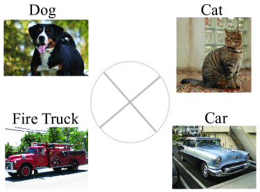
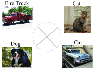
Permutation We provide an example to give the insight of Symmetric Generalization of Permutation. Consider a Grassmannian Frame living in , it resembles a cross (Theorem III.1 of Benedetto and Kolesar (2006)). As shown in Figure.1(a), there are four classes that correspond to different feature . Obviously, since Dog and Cat look similar to each other, they deserve to have a smaller margin in the feature space (near to each other). The same goes for the other two categories. However, if we swap the features of Truck and Dog to increase the distance between dogs and cats, as shown in Figure.1(b), the semantic relationship in the feature space would be disrupted. We argue that this can harm the model’s training and lead to worse generalization.
Rotation Symmetric Generalization of Rotation has been completely beyond our initial expectation. We believe that the margin or correlation between features is the most effective tool to understand NeurCol phenomenon. However, it fails to explain why different directions of features have different generalization. In Deep Learning community, Implicit Bias phenomenon is a possible way to approach this finding. Soudry et al. (2018) has proved that the Gradient Descent optimization leads to weight direction that maximizes the margin when using logistic loss and linear models. As a further progress, Lyu and Li (2020) extends this result to homogeneous neural networks. We speculate that the explanations for Symmetric Generalization of Rotation may be hidden within the layers of neural networks. Therefore, studying the Implicit Bias of deep models layer by layer could be a promising direction for future research. This is beyond the scope of our current work, and we leave it as a topic for our future work.
5 Conclusion
In this paper, we justify Generalized Neural Collapse hypothesis by leading to Grassmannian Frame into classification problems, which does not assume specific numbers of classes feature dimensions, and every two vectors in it can achieve maximal distances on a sphere. In addition, awaring that Grassmannian Frame is symmetric geometrically, we propose a question: is generalization of the model invariable to symmetric transformations of Grassmannian Frame? To explore this question, we conduct a series of empirical and theoretical analysis, and finally find Symmetric Generalization phenomenon. This phenomenon suggests that the generalization of a model is influenced by geometric invariant transformations of the Grassmannian Frame, including and .
References
- Papyan et al. [2020] Vardan Papyan, XY Han, and David L Donoho. Prevalence of neural collapse during the terminal phase of deep learning training. Proceedings of the National Academy of Sciences, 117(40):24652–24663, 2020.
- Ji et al. [2022] Wenlong Ji, Yiping Lu, Yiliang Zhang, Zhun Deng, and Weijie J Su. An unconstrained layer-peeled perspective on neural collapse. In International Conference on Learning Representations, 2022. URL https://openreview.net/forum?id=WZ3yjh8coDg.
- Fang et al. [2021] Cong Fang, Hangfeng He, Qi Long, and Weijie J Su. Exploring deep neural networks via layer-peeled model: Minority collapse in imbalanced training. Proceedings of the National Academy of Sciences, 118(43):e2103091118, 2021.
- Zhu et al. [2021] Zhihui Zhu, Tianyu Ding, Jinxin Zhou, Xiao Li, Chong You, Jeremias Sulam, and Qing Qu. A geometric analysis of neural collapse with unconstrained features. Advances in Neural Information Processing Systems, 34:29820–29834, 2021.
- Zhou et al. [2022a] Jinxin Zhou, Chong You, Xiao Li, Kangning Liu, Sheng Liu, Qing Qu, and Zhihui Zhu. Are all losses created equal: A neural collapse perspective. In Advances in Neural Information Processing Systems, volume 35, pages 31697–31710. Curran Associates, Inc., 2022a.
- Yaras et al. [2022a] Can Yaras, Peng Wang, Zhihui Zhu, Laura Balzano, and Qing Qu. Neural collapse with normalized features: A geometric analysis over the riemannian manifold. In Advances in Neural Information Processing Systems, volume 35, pages 11547–11560. Curran Associates, Inc., 2022a.
- Han et al. [2022] X.Y. Han, Vardan Papyan, and David L. Donoho. Neural collapse under MSE loss: Proximity to and dynamics on the central path. In International Conference on Learning Representations, 2022. URL https://openreview.net/forum?id=w1UbdvWH_R3.
- Tirer and Bruna [2022] Tom Tirer and Joan Bruna. Extended unconstrained features model for exploring deep neural collapse. In International Conference on Machine Learning, pages 21478–21505. PMLR, 2022.
- Zhou et al. [2022b] Jinxin Zhou, Xiao Li, Tianyu Ding, Chong You, Qing Qu, and Zhihui Zhu. On the optimization landscape of neural collapse under mse loss: Global optimality with unconstrained features. In International Conference on Machine Learning, pages 27179–27202. PMLR, 2022b.
- Mixon et al. [2020] Dustin G Mixon, Hans Parshall, and Jianzong Pi. Neural collapse with unconstrained features. arXiv preprint arXiv:2011.11619, 2020.
- Poggio and Liao [2020] Tomaso Poggio and Qianli Liao. Explicit regularization and implicit bias in deep network classifiers trained with the square loss. arXiv preprint arXiv:2101.00072, 2020.
- Graf et al. [2021] Florian Graf, Christoph Hofer, Marc Niethammer, and Roland Kwitt. Dissecting supervised contrastive learning. In International Conference on Machine Learning, pages 3821–3830. PMLR, 2021.
- Lu and Steinerberger [2022] Jianfeng Lu and Stefan Steinerberger. Neural collapse under cross-entropy loss. Applied and Computational Harmonic Analysis, 59:224–241, 2022.
- Liu et al. [2023] Weiyang Liu, Longhui Yu, Adrian Weller, and Bernhard Schölkopf. Generalizing and decoupling neural collapse via hyperspherical uniformity gap. In The Eleventh International Conference on Learning Representations, 2023.
- Yang et al. [2022] Yibo Yang, Shixiang Chen, Xiangtai Li, Liang Xie, Zhouchen Lin, and Dacheng Tao. Inducing neural collapse in imbalanced learning: Do we really need a learnable classifier at the end of deep neural network? In Advances in Neural Information Processing Systems, volume 35, pages 37991–38002. Curran Associates, Inc., 2022.
- Casazza and Kutyniok [2012] Peter G Casazza and Gitta Kutyniok. Finite frames: Theory and applications. Springer, 2012.
- Casazza and Kovačević [2003] Peter G Casazza and Jelena Kovačević. Equal-norm tight frames with erasures. Advances in Computational Mathematics, 18:387–430, 2003.
- Ambrus et al. [2021] Gergely Ambrus, Bo Bai, and Jianfeng Hou. Uniform tight frames as optimal signals. Advances in Applied Mathematics, 129:102219, 2021.
- Holmes and Paulsen [2004] Roderick B Holmes and Vern I Paulsen. Optimal frames for erasures. Linear Algebra and its Applications, 377:31–51, 2004.
- Strohmer and Heath Jr [2003] Thomas Strohmer and Robert W Heath Jr. Grassmannian frames with applications to coding and communication. Applied and computational harmonic analysis, 14(3):257–275, 2003.
- Welch [1974] Lloyd Welch. Lower bounds on the maximum cross correlation of signals (corresp.). IEEE Transactions on Information theory, 20(3):397–399, 1974.
- Shannon [1959] Claude E Shannon. Probability of error for optimal codes in a gaussian channel. Bell System Technical Journal, 38(3):611–656, 1959.
- Yaras et al. [2022b] Can Yaras, Peng Wang, Zhihui Zhu, Laura Balzano, and Qing Qu. Neural collapse with normalized features: A geometric analysis over the riemannian manifold. In Advances in Neural Information Processing Systems, volume 35, pages 11547–11560. Curran Associates, Inc., 2022b.
- Conway and Sloane [2013] John Horton Conway and Neil James Alexander Sloane. Sphere packings, lattices and groups, volume 290. Springer Science & Business Media, 2013.
- F.R.S. [1904] J.J. Thomson F.R.S. Xxiv. on the structure of the atom: an investigation of the stability and periods of oscillation of a number of corpuscles arranged at equal intervals around the circumference of a circle; with application of the results to the theory of atomic structure. The London, Edinburgh, and Dublin Philosophical Magazine and Journal of Science, 7(39):237–265, 1904. doi: 10.1080/14786440409463107.
- Conway et al. [1996] John H Conway, Ronald H Hardin, and Neil JA Sloane. Packing lines, planes, etc.: Packings in grassmannian spaces. Experimental mathematics, 5(2):139–159, 1996.
- Leng and Han [2011] Jinsong Leng and Deguang Han. Optimal dual frames for erasures ii. Linear Algebra and its Applications, 435(6):1464–1472, 2011. ISSN 0024-3795. doi: https://doi.org/10.1016/j.laa.2011.03.043.
- Lopez and Han [2010] Jerry Lopez and Deguang Han. Optimal dual frames for erasures. Linear Algebra and its Applications, 432(1):471–482, 2010. ISSN 0024-3795. doi: https://doi.org/10.1016/j.laa.2009.08.031.
- Kakade et al. [2008] Sham M Kakade, Karthik Sridharan, and Ambuj Tewari. On the complexity of linear prediction: Risk bounds, margin bounds, and regularization. In Advances in Neural Information Processing Systems, volume 21. Curran Associates, Inc., 2008.
- Bartlett and Mendelson [2002] Peter L Bartlett and Shahar Mendelson. Rademacher and gaussian complexities: Risk bounds and structural results. Journal of Machine Learning Research, 3(Nov):463–482, 2002.
- Bodmann and Paulsen [2005] Bernhard G Bodmann and Vern I Paulsen. Frames, graphs and erasures. Linear algebra and its applications, 404:118–146, 2005.
- Krizhevsky [2009] Alex Krizhevsky. Learning multiple layers of features from tiny images. 2009.
- He et al. [2016] Kaiming He, Xiangyu Zhang, Shaoqing Ren, and Jian Sun. Deep residual learning for image recognition. In Proceedings of the IEEE conference on computer vision and pattern recognition, pages 770–778, 2016.
- Simonyan and Zisserman [2014] Karen Simonyan and Andrew Zisserman. Very deep convolutional networks for large-scale image recognition. arXiv preprint arXiv:1409.1556, 2014.
- Huang et al. [2017] Gao Huang, Zhuang Liu, Laurens Van Der Maaten, and Kilian Q Weinberger. Densely connected convolutional networks. In Proceedings of the IEEE conference on computer vision and pattern recognition, pages 4700–4708, 2017.
- Deng et al. [2009] Jia Deng, Wei Dong, Richard Socher, Li-Jia Li, Kai Li, and Li Fei-Fei. Imagenet: A large-scale hierarchical image database. In 2009 IEEE conference on computer vision and pattern recognition, pages 248–255. Ieee, 2009.
- Benedetto and Kolesar [2006] John Benedetto and Joseph Kolesar. Geometric properties of grassmannian frames for r2 and r3. EURASIP Journal on Advances in Signal Processing, 2006, 12 2006. doi: 10.1155/ASP/2006/49850.
- Soudry et al. [2018] Daniel Soudry, Elad Hoffer, and Nathan Srebro. The implicit bias of gradient descent on separable data. In International Conference on Learning Representations, 2018. URL https://openreview.net/forum?id=r1q7n9gAb.
- Lyu and Li [2020] Kaifeng Lyu and Jian Li. Gradient descent maximizes the margin of homogeneous neural networks. In International Conference on Learning Representations, 2020. URL https://openreview.net/forum?id=SJeLIgBKPS.
- Xie et al. [2022] Liang Xie, Yibo Yang, Deng Cai, and Xiaofei He. Neural collapse inspired attraction-repulsion-balanced loss for imbalanced learning. Neurocomputing, 527:60–70, 2022.
- Yang et al. [2023] Yibo Yang, Haobo Yuan, Xiangtai Li, Zhouchen Lin, Philip Torr, and Dacheng Tao. Neural collapse inspired feature-classifier alignment for few-shot class-incremental learning. In The Eleventh International Conference on Learning Representations, 2023. URL https://openreview.net/forum?id=y5W8tpojhtJ.
- Yang et al. [2021] Zhiyong Yang, Qianqian Xu, Shilong Bao, Xiaochun Cao, and Qingming Huang. Learning with multiclass auc: theory and algorithms. IEEE Transactions on Pattern Analysis and Machine Intelligence, 44(11):7747–7763, 2021.
- Kulkarni and Posner [1995] Sanjeev R Kulkarni and Steven E Posner. Rates of convergence of nearest neighbor estimation under arbitrary sampling. IEEE Transactions on Information Theory, 41(4):1028–1039, 1995.
- Vural and Guillemot [2017] Elif Vural and Christine Guillemot. A study of the classification of low-dimensional data with supervised manifold learning. The Journal of Machine Learning Research, 18(1):5741–5795, 2017.
- Lezcano Casado [2019] Mario Lezcano Casado. Trivializations for gradient-based optimization on manifolds. Advances in Neural Information Processing Systems, 32, 2019.
- Lezcano-Casado and Martınez-Rubio [2019] Mario Lezcano-Casado and David Martınez-Rubio. Cheap orthogonal constraints in neural networks: A simple parametrization of the orthogonal and unitary group. In International Conference on Machine Learning, pages 3794–3803. PMLR, 2019.
Appendix A Related Work
Neural Collapse (NeurCol) was first observed by Papyan et al. [2020] in ., and it has since sparked numerous studies investigating deep classification models.
Many of these studies Ji et al. [2022], Fang et al. [2021], Zhu et al. [2021], Zhou et al. [2022a], Yaras et al. [2022a] have focused on the optimization aspect of NeurCol, proposing various optimization models and analyzing them. For example, Zhu et al. [2021] proposed Unconstrained Feature Models and provided the first global optimization analysis of NeurCol, while Fang et al. [2021] proposed Layer-Peeled Model, a nonconvex yet analytically tractable optimization program, to prove NeurCol and predict Minority Collapse, an imbalanced version of NeurCol. Other studies have explored NeurCol under Mean Square Error Loss (MSE) Han et al. [2022], Tirer and Bruna [2022], Zhou et al. [2022b], Mixon et al. [2020], Poggio and Liao [2020]. For instance, Han et al. [2022], Tirer and Bruna [2022] justified NeurCol under the MSE loss. In addition to MSE loss, Zhou et al. [2022a] extended such results and analyses a broad family of loss functions including commonly used label smoothing and focal loss. Besides, NeurCol phenomenon also inspires design of loss function in imbalanced learning Xie et al. [2022] and Few-Shot Learning Yang et al. [2023].
Previous studies on NeurCol have generally assumed that the number of classes is less than the feature dimension, and this assumption has not been questioned until recently. In the 11th International Conference on Learning Representations (ICLR 2023), Liu et al. [2023] proposed the Generalized Neural Collapse hypothesis, which removes this restriction by extending the ETF structure to Hyperspherical Uniformity. In this paper, we contribute to this area by proving the Generalized Neural Collapse hypothesis and introducing the Grassmannian Frame to better understand the NeurCol phenomenon.
Appendix B Proof of Theorem.3.1
We introduce this lemma:
Lemma B.1.
Suppose that , and that is a closed set. Suppose , we have:
This lemma can establish the relationship between geometry and probability. Then we start our proof.
See 3.1
Proof.
First, let us think about what kind of decoding is optimal. According to Shannon [1959], since the gaussian density is monotone decreasing with distance, an optimal decoding system for gaussian channel is the minimum distance decoding,
where is the prediction result. we consider the two-classes communication problem: there is only two number and transmitted. We denote the event that a signal is recover as as , then
According to Lemma.B.1, we have
For all numbers transmitted, the error event could be devided into the error event between every two numbers,
So
To obtain the code with minimal error probability, we can maximize . With a norm constraint for every code, we have
∎
Appendix C Proof of Theorem.3.2
In this section, we prove Theorem.3.2. Here are two lemmas that we are going to use.
C.1 Lemmas
Lemma C.1 (Lemma.7 of Yang et al. [2021]: Lipschitz Properties of Softmax).
Given , the function is defined as
then the function is -Lipschitz continuous.
Lemma C.2.
Given any matrix with constant on the diagonals and constant on off diagonals,
then we have .
Proof.
-
step1: Subtract the first rows by the last row.
-
step2: Add the first columns on the last column.
∎
C.2 Background
In the proof of Theorem.3.2, the techniques that we used is mainly limit analysis, and in addition a little linear algebra.
C.2.1 Assumption
We make the following assumption:
Assumption C.3.
In update of (4), parameters is properly selected: . In addition, is small enough to assure the system would converge and the norms of every vector in is always bounded by .
This small enough is necessary and reasonable for the convergce of Gradient Descent. With this assumption, we can assure that every variables in system (4) would not blow up and finally converge to a stable state. And the condition is to make sure both classifiers and features can be bounded by the same maximal norm.
C.2.2 Symbol Regulations
We regulate our symbols for clearer representation. Recall our setting, we use to denote the -th smaple in class and every class has samples. Here, we put -th sample in all class together, denote it as ,
Then we denote confidence probability of given by classifier as
where transform the into a probability vector. Refer to Lemma.C.1 for definition of .
C.2.3 Proof Sketch
We prove Theorem.3.2 by proving three Lemmas:
Lemma C.4 (Variability within Classes).
Lemma C.5 (Convergence to Self Duality).
Lemma C.6 (Convergence to Grassmannian Frame).
Consider the function (1), given any sequence , if as , then and would converge to the solution of
Obviously, Lemma.C.4 and Lemma.C.5 can directly indicate NC1 and NC2. We first prove them, which show the aggregation effect of cross entropy loss: features / linear classifier with the same class converge to the same point. Then NC4 is obvious under the conclusions of Lemma.C.4 and Lemma.C.5. Lemma.C.6 is the key step to prove that (1) converges to the min-max optimization as converge to zero. However, we still need to combine all Lemmas to obtain the minimized maximal correlation characteristic. Here is the proof:
Proof of (NC3).
First, we know
while Lemma.C.6 establishes a bridge between (1) and the following max-min problem:
According to Lemma.C.4 and C.5, we know the solution of (3) converge to
| (5) |
and there must exist a such that
| (6) |
Therefore, we substitute (5) and (6) into max-min:
where symbol in above equation means the solution of these optimization problems would converge to the same. min-max is exactly our expectant minimized maximal correlation characteristic. To ensure the establishment of above equivalence, is required to meet . ∎
C.2.4 Gradient Calculation
Before starting our proof, we calculate the gradient of (3) in terms of features and classifiers :
Then we turn it into the matrix form by arranging in every column.
| (7) | ||||
C.3 Proof of Lemma.C.4
See C.4
C.4 Proof of Lemma.C.5
See C.5
Proof.
According to the update rule (4) and gradient (7), for any , we have
Then, we bound :
| (8) | ||||
Then we use the assumption that , and consider and (c) separately.
| (a) | (9) | |||
| (b) | ||||
| (c) |
Then we combine (a) and (b):
| (10) | ||||
Next, we plug (9) and (10) into (8) to derive
Then we bound and .
For (A.1), we have
where the first inequality is because the function is -Lipschitz-continuous, and the last inequality follows from the bounded norm of : , we have . For (A.2), if , . If , we have
For (B), we have
The above final inequality is because both and can be seen as probability simplex, the norm of is always less than the norm of all-one matrix minus all-zero matrix, where the latter’s norm is . Finally, we can bound :
| (11) |
We put all and together to derive the difference inequality:
where
In above notation, the values of and refer to (11). We investigate if can converge to zero vector by adjusting . According to the Lemma.C.2, we know eigen values of are
Here, with properly selected parameters, we can make all eigen values of in . Therefore, as , and . ∎
C.5 Proof of Lemma.C.6
See C.6
Proof.
For simplicity, we leave out the upper script . First, we have
| (12) | ||||
In addition, we have
| (13) |
We denote as and define the margin of entire dataset (refer to Section.3.1 of Ji et al. [2022]) as follow:
Therefore, we have
| (14) |
where . Then we represent as the form of exponential function,
Denote the inverse function of as , where . Then continue from (14), we have
According to the monotonicity of , we have
Use the mean value theorem, there exists a such that
then
| (15) |
Then we will show . Since
we know and as . By simple calculation, we have and . Next, we denote the maximal norm at iteration as
Due to , . Then we devide on the both sides of (15) to obtain
therefore
So
The symbol in above equation means the solution of these optimization problems would converge to the same. ∎
Appendix D Proof of Theorem.3.8
Theorem D.1 (Theorem.5 of Kakade et al. [2008]: Margin Bound).
Consider a data space and a probability measure on it. There is a dataset that contains samples, which are drawn from . Consider an arbitrary function class such that we have , then with probability at least over the sample, for all margins and all we have,
Theorem.3.8 (Multiclass Margin Bound).
Consider a dataset with classes. For any classifier , we denote its margin between and classes as . And suppose the function space of the margin is , whose uppder bound is
Then, for any classifier and margins , the following inequality holds with probability at least
where
| empirical risk term | |||
| probability term |
is the Rademacher complexity Kakade et al. [2008], Bartlett and Mendelson [2002] of function space .
Proof.
First, we decompose the accuracy as accuracies within every class by Bayes Theory:
| (16) |
where is the probability density of -th class. Then, we focus on the accuracy within every class .
According to union bound, we have
Recall our assumption of function class:
Then follow from the Margin Bound (Theorem.D.1), we have
with probability at least . Then, we perform the following replace to drive the final result:
∎
Appendix E Proof of Theorem.4.2
We first introduce the definition of Covering Number.
Definition E.1 (Covering Number Kulkarni and Posner [1995]).
Given and , the open ball of radius around is denoted as
Then the covering number of a set is defined as the smallest number of open balls whose union contains :
The following conclusion is demonstrated in the proof of Theorem.1 of Kulkarni and Posner [1995]. We use it to prove our theorem.
Theorem E.2 (Vural and Guillemot [2017], Kulkarni and Posner [1995]).
There are samples drawn i.i.d from the probability measure . Suppose the bounded support of is , then if is larger then Covering Number , we have
where is the sample that is closest to in :
Then we provide the proof of Theorem.4.2.
See 4.2
Proof.
We decompose the accuracy:
| (17) |
where is the class distribution. Then, we focus on the accuracy within every class .
We select the data that is closest to in class samples , and denote it as
According to the linear separability,
For any , we have
| (18) | ||||
The prediction result is related to the distance between and . According to Theorem.E.2, we know
To obtain the correct prediction result, , assure for all , we choose . Therefore, we have
| (19) | ||||
Then using the conlcusions of NeurCol, if maximal norm is denoted as , we have
∎
Appendix F Some Details of Experiments
F.1 Training Detail
In the experiments of Section.4.2, we follow Papyan et al. [2020]’s practice. For all experiments, we minimize cross entropy loss using stochastic gradient descent with epoch , momentum , batch size and weight decay . Besides, the learning rate is set as and annealed by ten-fold at and epoch for every dataset. As for data preprocess, we only perform standard pixel-wise mean subtracting and deviation dividing on images. To achieve accuracy on training set, we only use RandomFilp augmentation.
F.2 Generation of Equivalent Grassmannian Frame
We use Code.1 to generate Equivalent Grassmannian Frame with different directions and orders. Note that the generation of rotation matrix uses the method of Lezcano Casado [2019], Lezcano-Casado and Martınez-Rubio [2019].
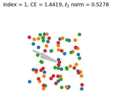
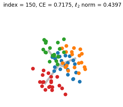
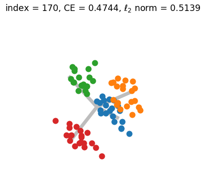
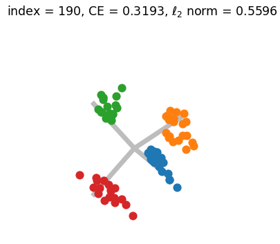
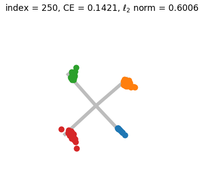
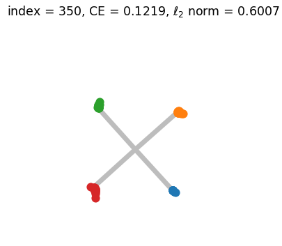
Appendix G Numerical Simulation and Visualization of Generalized Neural Collapse
Figure.2 shows the results of a numerical simulation experiment conducted to illustrate the convergence of Generalized Neural Collapse. A GIF version of Figure.2 can be found HERE. During the simulation, we discovered that the condition , which is believed to be necessary for the occurrence of Grassmannian Frame (in the NC3 of Theorem.3.2), may not be required. This suggests that there may be other ways to prove Generalized Neural Collapse with fewer assumptions.