A study on a minimally broken residual TBM-Klein symmetry with its implications on flavoured leptogenesis and ultra high energy neutrino flux ratios
Abstract
We present a systematic study on minimally perturbed neutrino mass matrices which at the leading order give rise to Tri-BiMaximal (TBM) mixing due to a residual Klein symmetry in the neutrino mass term of the low energy effective seesaw Lagrangian. Considering only the breaking of with two relevant breaking parameters (), after a comprehensive numerical analysis, we show that the phenomenologically viable case in this scenario is a special case of TM1 mixing. For this class of models, from the phenomenological perspective, one always needs large breaking (more than ) in one of the breaking parameters. However, to be consistent the maximal mixing of , while more than breaking is needed in the other, a range and could be probed allowing breaking up to in the same parameter. Thus though this model cannot distinguish the octant of , non-maximal mixing is preferred from the viewpoint of small breaking. The model is also interesting from leptogenesis perspective. Unlike the standard -leptogenesis scenario, here all the RH neutrinos contribute to lepton asymmetry due to the small mass splitting controlled by the breaking parameters. Inclusion of flavour coupling effects (In general, which have been partially included in all the leptogenesis studies in perturbed TBM framework) makes our analysis and results pertaining to a successful leptogenesis more accurate than any other studies in existing literature. Finally, in the context of recent discovery of the ultra high energy (UHE) neutrino events at IceCube, assuming UHE neutrinos originate from purely astrophysical sources, we obtain prediction on the neutrino flux ratios at neutrino telescopes.
1 Introduction
The structure of the leptonic mixing matrix has always been the center of attraction in the flavour model
building landscape. Until the experimental discovery of a nonvanishing value of the reactor mixing angle
[1, 2], it was the paradigm of Tri-BiMaximal (TBM) Ansatz of
[3], that dominated almost for a decade[4] with the
prediction , particularly in the approaches of model building with the discrete non-Abelian
symmetries such as , etc.[5]. Now the neutrino mixing parameters, particularly
two mass squared differences and three mixing angles have entered in the precision era. Thus, as far as the TBM mixing
is concerned, it has been rendered outdated at least by the nonvanishing value of . However, due to its other
two predictions, and which are still close to their respective experimental
best-fit values, the TBM mixing cannot be just overthrown from the way in search for an viable flavour model of
neutrino masses and mixing. Several theories for the modification of TBM mixing in terms of perturbations to the TBM
mass matrix have been proposed [6, 7]. A brief recall of few of the existing theories which deal with schemes of the modified TBM mixing would be worthwhile in our context. Ref.[6] has discussed the
consequences of perturbation to the effective but with less emphasis on the high energy symmetries.
On the other hand, in some of the works in Ref.[7], a high energy symmetry group is perturbed
softly such that the effective residual symmetries are unable to generate the exact TBM mixing. Alternative moderated versions, such as
TM1[8, 9], TM2[8, 10] mixing with an additional prediction
on the Dirac CP phase , have also been considered to comply with the existing neutrino oscillation data. Elaborate descriptions of direct models mainly focusing on TM1 and TM2 mixings have been given in references [11] and [12].
Besides all these, there exists a residual symmetry approach[13, 14, 15, 16, 17]. In [13, 14, 15] it has been shown
that a neutrino Majorana mass matrix with nondegenerate eigenvalues always enjoys
a residual Klein symmetry accompanied with a diagonal charged lepton
mass matrix which is further protected by a symmetry for . Thus, given a neutrino mixing
matrix, one can always construct the corresponding residual Klein symmetry generators for each of
the symmetries. For a mixing of TBM kind, these generators are found to be identical to the generators
of the group in a three dimensional irreducible representation[15].
The diagonal type symmetry acts as the residual symmetry in the charged lepton sector
while the other two generate a TBM-Klein symmetry with one of them being the interchange
symmetry[18]. In[19], the consequences of a Scaling-Klein symmetry have also been worked out.
It is clear that the vanishing value of in TBM mixing is caused due to the existence of the interchange symmetry as one of the TBM-Klein symmetry generators. Thus to be consistent with the oscillation data, one has to relax the constraints arising from the exact symmetry. One way is to consider a flavoured nonstandard CP symmetry ()[20] instead of an exact symmetry with the other TBM-Klein generator being completely broken. Introduction of such a symmetry leads to a co-bimaximal (, ) mixing[21]. This approach has drawn a lot of attention[22] after the recent hint from T2K about a maximal Dirac CP violation[23]. Following this approach, alternatives to TBM mixing have been proposed recently in[24] and [25]. In both the papers, the interchange symmetry has been replaced by a CP symmetry keeping the remaining generator of the TBM-Klein symmetry intact. This further makes the more predictive with the added predictions of the unbroken TBM generator. In our present work we follow this direction, i.e., we keep a generator of the residual TBM-Klein symmetry unbroken and study modifications of the interchange symmetry. However, instead of replacing the interchange symmetry by , we have shown how minimal the breaking of the former could be to be consistent with the recent global fit neutrino oscillation data[26] or in other words, we have performed a study on the goodness of the symmetry while keeping the other of the TBM-Klein symmetry unbroken. Unlike in [24, 25], here a nonmaximal value of is also allowed. We show that among the two relevant breaking parameters, one should always be large (more than 0.45). However, to be consistent with the other global fit data, whilst a maximality or a near maximality in requires large breaking (more than 0.35) in the other, a range or could be probed if we allow the same breaking parameter up to 0.25 (to be consistent with neutrino oscillation global fit data, at least breaking of the symmetry is required in our scenario). Thus our model could be tested shortly in the experiments such as NOA[27]. We have studied the breaking of the interchange symmetry from the Lagrangian level of the Type-I seesaw. This in turn has allowed us to explore a scenario of leptogenesis with quasi-degenerate heavy RH neutrinos and to work out the consequences pertaining to a successful leptogenesis in this scheme.
Without loss of any generality we choose to work in the diagonal basis of charged leptons where the right handed neutrino mass matrix is also diagonal unless it is perturbed. The Lagrangian for the neutrino mass terms (Dirac+Majorana) is denoted as
| (1.1) |
where is the SM lepton doublet of flavour . The effective light neutrino mass matrix is then given by the well known Type-I seesaw formula
| (1.2) |
A unitary matrix diagonalizes in (1.2) as
| (1.3) |
where are real positive mass eigenvalues of light neutrinos. Since is diagonal, is simply equivalent to the leptonic mixing matrix :
| (1.4) |
where is an unphysical diagonal phase matrix and , with the mixing angles . Here we have followed the PDG convention[28] but denote our Majorana phases by and . CP-violation enters in the leptonic sector through nontrivial values of the Dirac phase and Majorana phases with .
We first derive the constraint equations emerging from a residual Klein symmetry in the case of a general interchange symmetry and then discuss the implications of those equations to the TBM mixing scheme plus the related modifications. The unbroken TBM generator in this scenario leads to a TM1 and a TM2 type mixing[8]. Since the predicted solar mixing angle () for a TM2 type mixing is disfavored at [26], we devote our entire numerical section only to the TM1 type scenario arising in our analysis. Notice that, though the unbroken leads to a TM1 type mixing, here the existence of another partially broken symmetry makes this scenario more predictive than the pure TM1.
Predominance matter over antimatter has become a proven fact by several experimental observations. All our known structures of universe (like stars, galaxies and clusters) are made up of matter, where as existence of antimatter hasn’t been confirmed yet. The dynamical process of generation of baryon asymmetry from baryon symmetric era of early Universe is known as baryogenesis. Among the various possible mechanisms of baryogenesis, the most interesting and also relevant to our present neutrino mass model is baryogenesis through leptogenesis. For successful generation of baryon asymmetry Sakharov conditions[29] must be satisfied. The necessary CP violation is provided by the complex Yukawa coupling between heavy singlet right handed neutrinos and left handed doublet neutrinos. Existence of Majorana mass term of the right handed neutrinos ensures lepton number violation. Departure from thermal equilibrium is achieved whenever the interaction rate of Yukawa coupling is smaller than the Hubble expansion rate. Thus the model under consideration possesses all the necessary ingredients to satisfy Sakharov conditions and is able to produce lepton asymmetry at a very high scale which is further converted into baryon asymmetry through Sphaleronic transitions.
In this work we examine qualitatively as well as quantitatively, how efficiently our model can address
the low energy neutrino phenomenology and cosmological baryon asymmetry within the same frame work. Therefore
Lagrangian parameters once constrained by the oscillation data are used thereafter in the computations of
leptogenesis in a bottom up approach. Since we plan to study leptogenesis over a wide range of right handed neutrino mass, we explore the
possibilities of both flavour dependent and flavour independent leptogenesis. To track the evolution of the baryon asymmetry
from very high temperature down to very low temperature (present epoch) we use network of most general flavour
dependent coupled Boltzmann Equations (BEs) where contributions from all three generations of RH neutrinos
are taken into account. Implications of nondiagonal right handed neutrino mass matrix have also been dealt with great care.
Recently IceCube detector[30, 31] at the south pole has detected ultra high energy (UHE ) neutrino events which in turn has opened a new era in neutrino astronomy. Though the present data points those neutrinos to be of extraterrestrial origin, the sources of those neutrinos are still unknown. Assuming the sources to be pure astrophysical (we consider the conventional and sources), we calculate the flavour ratios at the neutrino telescope. Due to the broken symmetry in this model, commonly predicted democratic flavour distribution 1:1:1 changes. Thus the prediction of the flavour ratios in this model will be tested hopefully with enhanced statistics in neutrino telescopes such as IceCube.
So, the main and new features of this work could be summarised as follows:
i) Unlike the previous literatures, the model under consideration deals with neither arbitrarily broken TBM [6] nor an exact
TM1 mixing[8, 9, 11, 12]. To be precise, for an arbitrarily broken TBM, both the symmetries in
are broken softly[6] whereas, for an exact or pure TM1 mixing,
is broken completely while the other remains unbroken. In our scenario, similar
to pure TM1 mixing, we keep unbroken, however, instead of breaking completely,
we restrict to the fact that how minimal the breaking of the could be to be consistent with the existing
neutrino data. Thus the scenario is a special case of a pure TM1 mixing and is more predictive than the said mixing due the
existence of another partially broken . This separates our work from any previous analysis and thus after
constraining the model parameter space with neutrino oscillation data, whatever predictions emerge, are entirely novel.
Though Ref.[32], and Ref.[33] share some common ground with this work, we shall point out the distinction
in the numerical section where we present a comparative study of this work with the works which look similar a priory.
ii) For the numerical analysis, we perform an exact diagonalization of the neutrino mass matrix which in turn
allows us to take into consideration the
terms which are higher order in the breaking parameters (terms proportional to and so on are usually neglected in perturbed TBM analysis).
Thus our numerical results are quite robust. If we allow breaking in one of the relevant breaking parameters up to , our minimal breaking scenario prefers non-maximal mxing, e.g., within the range and hence a particular range of the Dirac CP phase , due an analytical correlation predicted by the unbroken (though this correlation is also present in case of a pure TM1 mixing). Thus the goodness of this scenario can easily be tested in the ongoing and forthcoming neutrino experiments.
iii) Within the broken TBM scenarios, in general baryogenesis via leptogenesis has been studied assuming -dominated scenario where the
heavy neutrino flavour effects are neglected, assuming any asymmetry produced by the heavier neutrinos are significantly washed out
by and -washout do not affect asymmetry produced by at the production. In addition, to compute the final , approximate
formulae are used which include partial flavour coupling effects (an assumption of ‘’ matrix to be diagonal). In our scenario,
due to the typical structure of the symmetry, the RH neutrino masses are very close to each other which compels us to take into account the
effects of as well as . We solve full flavour dependent Boltzmann equations with full flavour coupling effects and show
how depending upon breaking parameters the next to lightest of the heavy RH neutrinos affects the final asymmetry. With best of our
knowledge, within the broken TBM framework, such a diligent computation of leptogenesis has not been done before.
iv) Encouraged by the recent discovery of high energy neutrino events at IceCube, we calculate flavour flux ratios at neutrino telescopes
which deviates from the democratic flavour distribution 1:1:1. The predicted flavour flux ratios are either testable with enhanced statistics
at the neutrino telescopes such as IceCube or could be used as an input to the astrophysical fits [34] to the existing data to test this model.
v) This model also predicts a testable range of the neutrino less double beta decay parameter .
The rest of the paper is organized as follows: In Sec.2, we briefly review the basic framework of residual symmetry along with a discussion on the general interchange symmetry which is characterized by a residual Klein symmetry. Given the general setup in Sec.2, we further focus on the TBM mixing () and phenomenologically consistent minimal breaking pattern of the residual in Sec.3. Sec.4 is entirely devoted to the study of generation of baryon asymmetry through leptogenesis. Its various subsections deal with rigorous evaluation of CP asymmetry parameters, setting up the chain of Boltzmann equations applicable in different temperature regimes. The extensive numerical study of the viable cases (which includes : constraining the parameters by global fit of oscillation data, computation related to the baryogenesis via leptogenesis and prediction of the flavour flux ratios at the neutrino telescopes) is given in Sec.5. In Sec.6, we summarize the entire work and try to highlight the salient features of this study towards addressing neutrino oscillation phenomenology along with major issues such as baryon asymmetry of universe.
2 Residual symmetry and its implication on variants
A horizontal symmetry of a neutrino mass matrix is realized through the invariance equation
| (2.1) |
where is an unitary matrix in the neutrino flavour space. Now Eq.(2.1) and (1.3) together imply that we can define a new unitary matrix such that it also diagonalizes . The matrix should then be equal to :
| (2.2) |
with being a diagonal rephasing matrix. For neutrinos of Majorana type, . Therefore, can only have
entries . Thus there are now eight possible structures of two of which are a simple unit matrix and its negative.
The remaining six can be considered as three different pairs, where the two matrices of a pair are identical to
each other apart from an overall relative negative sign.
Finally, among these three (pairs)
matrices, only two are independent as each always satisfies the relation , where and can take
value 1, 2 and 3. Now implies each define a symmetry. Therefore, on account of the relation
in (2.2), each also represents symmetry and generates the
residual symmetry (Klein Symmetry) in the neutrino mass term of the Lagrangian. We can now choose the
two independent matrices as and
for . For , and would differ from the previous
choices only by an overall minus sign.
Given this basic set up, we first discuss the general interchange symmetry in the framework of residual . We then proceed to the discussion of TBM mixing by setting the solar mixing angle in the interchange scheme. A neutrino Majorana mass matrix
| (2.3) |
invariant under the interchange symmetry is diagonalized as
| (2.4) |
where
| (2.5) |
The parameter is related to the solar mixing angle as . Here we choose the appropriate minus signs in to be in conformity with the PDG convention[28]. Now from (2.2), and corresponding to and can be calculated as
| (2.6) |
The relation makes the construction of simple: . Thus will be of form
| (2.7) |
Since is basically the interchange symmetry in the flavour basis, we therefore rename the residual Klein symmetry for this interchange case as . We now implement the on the Dirac mass matrix and the Majorana mass matrix of (1.1) as
| (2.8) |
Equations in (2.8) automatically imply the invariance of and on account of the relation . Now one can work out the constraint equations that arise due the invariance relations in (2.8). A most general mass matrix
| (2.9) |
that is invariant under (cf. Eq. 2.8) would lead to the following constraint equations: for invariance,
| (2.10) |
for invariance,
| (2.11) |
and for invariance,
| (2.12) |
Note that since is a general complex matrix, one can simply consider the constraint equations derived in (2.10), (2.11) and (2.12). However, since is Majorana type, one has to consider a complex symmetric structure for the matrix in (2.9) which would require the replacements , and in the equations (2.10), (2.11) and (2.12). The invariance equations of (2.8) are the consequences of an assumed symmetry on both the left () and the right chiral () fields. It is worthwhile to highlight another interesting aspect of this symmetry. The overall invariance of the effective that arises from the Type-I seesaw mechanism, can be realized by implementing the residual on the left-chiral fields only. Since arises due to the seesaw relation in (1.2), the invariance condition on alone
| (2.13) |
implies
| (2.14) |
For such an invariance, the determinant of would be vanishing and therefore one of the neutrinos will become massless[33]. Proceeding in the similar manner, as in the previous case, we derive the following constraint equations for partial invariance (cf. Eq. 2.13). For invariance we have
| (2.15) |
Similarly for invariance
| (2.16) |
and for invariance
| (2.17) |
could be obtained. Again the minus signs in the invariance equations are used to be consistent with the PDG convention. Let us now switch to the analysis on TBM mixing which is a trivial generalization of the above discussion with . We write the generators for TBM mixing as
| (2.18) |
Similarly, for , the well known mixing simply comes out from (2.5) as
| (2.19) |
As mentioned in the introduction, since leads to a vanishing value , the
full can not be a phenomenologically accepted symmetry of the Lagrangian.
To be more precise, the nondegenarate eigenvalue of , i.e., , fixes the third
column of to which implies a vanishing value of while
a nonzero value of the latter has been confirmed by the experiments at [35].
Thus to generate a nonzero we break the () with small
breaking parameters keeping the other residual s (either or ) intact.
In the next section, depending upon the residual symmetries on the neutrino fields and their breaking pattern,
we categorize our discussion into three categories.
3 Breaking of : perturbation to the TBM mass matrices
The residual TBM-Klein symmetry is implemented in the basis where is diagonal. This further leads to degenerate heavy RH neutrinos. We then consider the most general perturbation matrix that breaks only the in . Since these breaking parameters are responsible for generation of nonzero , the extent of quasidegeneracy between the right handed neutrinos (or in other words the smallness of the breaking parameters) is now dictated by the value of . A systematic discussion of the breaking scheme is presented in the following subsections.
3.1 and on both the fields, and
Case 1. invariance of : breaking of in
At the leading order, i.e., when the effective light neutrino mass matrix respects exact TBM-Klein symmetry, the most general Dirac mass matrix and the Majorana mass matrix satisfy the invariance equations
| (3.1) |
Now using (2.10), (2.11) and (2.12) one constructs the structures and as
| (3.2) |
where are real positive numbers and are phase parameters. To generate a viable neutrino mixing we now consider breaking of in the RH Majorana mass matrix only. We modify by adding a complex symmetric perturbation matrix that breaks the but invariant under the transformation
| (3.3) |
to ensure the overall invariance of the effective light neutrino . Now with , (2.10) would imply that a general complex symmetric matrix
| (3.4) |
which is invariant under , follows the constraint equations
| (3.5) |
Note that and do not break the symmetry, thus for a simplified discussion we take both of them to be of vanishing values. Thus the perturbation matrix can be written as
| (3.6) |
Now the effective which is invariant under can be written as
| (3.7) |
where
| (3.8) |
Since invariance of the effective always fixes the first column of the mixing matrix to up to some phases, a direct comparison of the latter with the of (1.4) leads to the well known correlation between and for a TM1 mixing as
| (3.9) |
To introduce CP violation in a minimal way, it is useful to assume [36] in the matrix (Eq.(3.2)) which after the phase rotation , can be conveniently parametrized as
| (3.10) |
where . With the parametrization of of (3.8) as
| (3.11) |
where are dimensionless breaking parameters, we proceed further to calculate the effective light neutrino mass matrix (). Eq. (3.7) can now be simplified as
| (3.12) | |||||
where and , i.e a factor of is absorbed in the elements matrix however its structure is exactly identical with that of . To be precise, the modulus parameters , and are basically times the unprimed parameters , and respectively. Thus the elements of the matrix now become functions of total six parameters, mathematically which can be represented as
| (3.13) |
where . Explicit forms of different s are given in the Appendix A.1.
Case 2. invariance of : breaking of in
In this case we follow the similar prescription as considered in the previous case, i.e., along with the leading order invariance equations
| (3.14) |
we add a perturbation matrix to , where the former satisfies
| (3.15) |
Now (2.11) with and of (3.4) together lead to the constraint equations
| (3.16) |
Using the constraint relations in (3.16) we get invariant as
| (3.17) |
where are assumed to have vanishing values due to their blindness towards interchange symmetry. The effective which is now invariant under comes out as
| (3.18) |
where
| (3.19) |
Note that invariance of always fixes the second column of the mixing matrix to the second column of . This leads to the constraint relation between and as
| (3.20) |
Given a nonvanishing value of , the solar mixing angle is always greater than which is disfavored at 3 by the the present oscillation data[26]. Therefore, we do not consider this case in our numerical discussion.
3.2 on and on both the fields, and
Case 1. invariance of : breaking of in
In this case, for the effective to be invariant under and at the leading order, the constituent mass matrices follow the invariance equations given by
| (3.21) |
Now using (2.15) and (2.12), we find forms of the most general and that satisfy (3.21):
| (3.22) |
For the sake of simplicity, we assume and take out the phase through the rotation . Thus takes the form
| (3.23) |
where and , , are all real positive parameters. An arbitrary breaking perturbation matrix could be added to , since the overall invariance of the effective is independent of the form of the RH Majorana mass matrix. We choose the perturbation matrix to be
| (3.24) |
Thus the effective is calculated (using phase rotated of eq.(3.23) and broken symmetric ) as
| (3.25) |
Using the redefinition of the parameters as
| (3.26) |
(with , , ,, being real) the elements of matrix can be expressed as functions of .
Explicit functional forms for the elements matrix can be found in Appendix A.2.
In this case also, due to the invariance of , the relation between and
is same as that of (3.9). Another interesting point is that of (3.22) is of determinant zero due
to the imposed symmetry. Thus the matrix has one vanishing eigenvalue. Since
also fixes the first column of the mixing matrix, the vanishing eigenvalue has to be which is
allowed by the current oscillation data.
Case 2. invariance of : breaking of in
The effective to be invariant under and at the leading order, the constituent mass matrices follow the invariance equations
| (3.27) |
The most general Dirac mass matrix and the Majorana mass matrix that satisfy (3.27) are of the forms
| (3.28) |
where we have used (2.16) and (2.12) to find these forms. Similar to the previous case the effective can be calculated as
| (3.29) |
where
| (3.30) |
with being an arbitrary perturbation matrix. Here also due to the imposed symmetry, the matrix of (3.28) has zero
determinant which imply the matrix has one vanishing
eigenvalue. Since fixes the second column of the mixing matrix, the vanishing eigenvalue has to be
which is not allowed due to a positive definite value of the solar mass squared difference () for both normal and inverted hierarchy.
Therefore we discard this case in our analysis.
3.3 and on only
In this case the leading order transformations are
| (3.31) |
| (3.32) |
The most general effective for both the cases lead to two vanishing eigenvalues. Due to this degeneracy in masses, one can not fix the leading order mixing as the TBM mixing matrix, thus the residual symmetry approach breaks down (Due to the arbitrariness of the mixing matrix one cannot reconstruct the corresponding generators; the matrices). Therefore both of these cases are discarded in our analysis.
4 Baryogenesis through leptogenesis
Baryogenesis via leptogenesis is an excellent mechanism to understand the observed excess of baryonic matter over anti matter. The amount of baryon asymmetry is expressed by the parameter: ratio of difference in number densities of baryons and anti baryons to the entropy density of the universe. The experimentally observed value[37, 38] of this baryon asymmetry parameter is given by
| (4.1) |
with being the entropy density of the universe. In this mechanism, the CP violating and out of equilibrium decays of heavy RH neutrinos[39] create an excess lepton asymmetry which is further converted in to baryon asymmetry by nonperturbative sphalerons[40].
4.1 Calculation of CP asymmetry parameter
The part of our Lagrangian relevant to the generation of a CP asymmetry is
| (4.2) |
where is the left-chiral SM lepton doublet of flavour , while is the charge conjugated Higgs scaler doublet. It is evident from (4.2) that the decay products of can be and . We are interested in the flavour dependent CP asymmetry parameter which is given by
| (4.3) |
where is the corresponding partial decay width and in the denominator a sum over the flavour index has been considered. A nonvanishing value of requires the interference between the tree level and one loop decay contributions of , since the tree level decay width is given by
| (4.4) |
and thus leads to a vanishing CP violation. Before presenting the rigorous formulas of partial decay width and the CP asymmetry parameter, let us point out a subtle issue. Since the computations related to leptogenesis require the physical masses of the RH neutrinos, a nondiagonal RH neutrino mass matrix should be rotated to its diagonal basis. A Majorana type RH neutrino mass matrix could be put into diagonal form with a unitary matrix as
| (4.5) |
where are the eigenvalues of . Thus in the diagonal basis of , the Dirac neutrino mass matrix (the neutrino Yukawa couplings) also gets rotated as
| (4.6) |
where is the Dirac neutrino mass matrix in the nondiagonal basis of and is given by with being the VEV of the SM Higgs. Accordingly, the tree level decay width can now be calculated as
| (4.7) |
Along with (4.7), taking into account the contributions from one loop vertex and self energy diagrams and without assuming any hierarchy of the right handed neutrinos the most general expression (keeping upto fourth order of Yukawa coupling) of the flavour dependent CP asymmetry parameter [41] can be calculated as
| (4.8) | |||||
where 333It is to be noted that if the right handed neutrino mass matrix is taken to be diagonal then is a unit matrix and we would have and , where ., and is the loop function given by
| (4.9) |
In the expression of , the term proportional to arises from the one loop vertex term interfering with the tree level contribution. The rest are originating from interference of the one loop self energy diagram with the tree level term. It is also worth clarifying the reason behind the explicit flavour index ‘’ on the CP asymmetry parameter in (4.8). Depending upon the temperature regime in which leptogenesis occurs, lepton flavours may be fully distinguishable, partly distinguishable or indistinguishable[42]. Assuming leptogenesis takes place at , lepton flavours cannot be treated separately if the concerned process occurs above a temperature . If the said temperature is lower, two possibilities might arise. When GeV, all three () flavours are individually active and we need three CP asymmetry parameters for each generation of RH neutrinos. On the other hand when we have , only the -flavour can be identified while the and act indistinguishably. Here we need two CP asymmetry parameters and for each of the RH neutrinos. As an aside, let us point out a simplification for unflavoured leptogenesis which is relevant for the regime . Summing over all ,
| (4.10) |
i.e. the second term in the RHS of (4.8) vanishes. The flavour-summed CP asymmetry parameter is therefore given by the simplified expression
| (4.11) | |||||
It is evident from the thorough discussion of different types of breaking schemes presented in Sec.3, that only two of those may be compatible with the constraints of the neutrino oscillation data. Therefore while performing the computations of leptogenesis, we should take into account only those symmetry breaking patterns which at least have the potential to satisfy oscillation data and in present work those two theoretically relevant options are Case I of both Sec.3.1 and Sec.3.2. For the Case I in Sec.3.1, the RH neutrino mass matrix is diagonal in the TBM limit. However, for the realistic scenario, i.e., in the broken TBM frame work, is off diagonal. On the other hand, for the Case I in Sec.3.2, is always diagonal. For the time being, let us leave the latter case for the numerical section and discuss here the former, i.e., Case I belonging to Sec.3.1. Since right handed neutrino mass matrix is nondiagonal in this case, at first we have to diagonalize the matrix and find out the corresponding diagonalizing matrix which would be used thereafter to rotate the Dirac matrix . After a straight forward diagonalization of the matrix in (3.11), the eigenvalues come out to be
| (4.12) |
It is clear from (4.12) that the RH neutrino masses are very close to each other, separated only by the breaking parameters. This opens up a possibility of resonant enhancement of the CP asymmetry parameter which may yield the required value of baryon asymmetry at a very low mass scale. We have checked the condition for resonance444resonance in CP asymmetry parameters is achieved when very carefully and found that even for the lowest allowed (by oscillation data) value of the breaking parameters it is not possible the meet the resonant condition. This is since, given the neutrino oscillation data, the resonance condition in our model can be translated approximately to
| (4.13) |
where and is the mass scale of the RH neutrino while unperturbed. If one wants to achieve resonance, say at GeV, clearly, the scenario is inconsistent since in that case while as we shall see in the numerical section, the LHS of (4.13) is . Interestingly, in this way, we could also circumvent the effect of RH neutrino flavour oscillation[43] where the same resonance condition leads to an additional CP asymmetry produced by the RH neutrino flavour oscillation[48]. Nevertheless, since the RH neutrino masses are close to each other, we can not treat this scenario to be hierarchical where the asymmetries generated from the RH neutrinos of higher masses can be safely neglected[45]. Therefore we opt for the rigorous method of quasidegenerate leptogenesis where the contribution from all three right handed neutrinos are taken into account[41] and show how the produced asymmetry from each RH neutrino is affected by the other.
Since is a real matrix, the diagonalization matrix will also be a real. Thus is now an orthogonal matrix with its different elements in terms of the breaking parameters as
where
| (4.15) |
Unflavoured CP asymmetry parameter:
The expression of unflavoured CP asymmetry parameter in (4.11) involves the matrix which can further be written as
| (4.16) |
Taking into account the explicit form of given in (3.10), different elements of the can be written as
| (4.17) |
It is clear from the above set of equations that is completely real matrix which in turn dictates that is also a real matrix due to the real nature of the matrix . Since the CP asymmetry parameter in (4.11) is proportional to , it can easily be inferred that generation of lepton asymmetry is not at all possible in the unflavoured regime. Now our task is to examine whether we can have nonvanishing values of flavour dependent CP asymmetry parameters so that we can get generate baryon asymmetry in the fully flavoured or partly flavoured regime.
Flavour dependent CP asymmetry parameters:
The flavoured CP asymmetry parameters of (4.8) can be represented in a little bit simpler form as
| (4.18) | |||||
where and . The in (4.18) can further be simplified as
| (4.19) |
Although matrix is a real matrix, matrix contains complex parameters. Since contains individual elements of matrix, we would have a nonzero imaginary part which leads to a nonvanishing flavoured CP asymmetry parameters and thus nonzero . The full functional forms of these flavoured CP asymmetry parameters () in terms of parameters of matrix and the symmetry breaking parameters would be too cumbersome to present here. We calculate all nine of them and use in the Boltzmann equations suitably. Nevertheless, to realize the significance of the phase parameter , it is useful to simplify further the expression of . For this, let us focus on the first term (the second term would be treated in the same manner) in the RHS of (4.18)
| (4.20) |
It is to be noted that the phase parameter is contained in the unprimed matrices (). The diagonalization matrix doesn’t depend on . Now matrix possesses the phase in its off-diagonal elements in form of . Therefore inversion of sign of will not affect sign of . A closer inspection of the elements of the matrix reveals that (for ) is bound to be function of which will appear in the expression of CP asymmetry parameters as an overall multiplicative factor. Thus we can say that phase dependence of the flavoured CP asymmetry parameters is of the form : . So is an odd function of the phase , i.e .
4.2 Boltzmann equations and baryon asymmetry in different mass regimes
For an evolution down to the electroweak scale, one needs to solve the corresponding Boltzmann Equations (BEs) for the number density of a particle type ‘a’ (in our context, either a right-chiral heavy neutrino or a left-chiral lepton doublet ). For this purpose it is convenient to define with , . We follow here the treatment given in Ref.[41]. The equations involve decay transitions between and as well as plus scattering transitions . Here represents the left-chiral quark doublet with and stands for either or . The number density of a particle of species and mass with internal degrees of freedom is given by[46]
| (4.21) |
being the modified Bessel function of the second kind with order 2. The corresponding equilibrium density is given by
| (4.22) |
Stage is now set up for the usage of the Boltzmann evolution equations given in Ref.[41] – generalized with flavour[47]. In making this generalization, one comes across a subtlety: the active flavour in the mass regime (given by the leptogenesis scale ) under consideration may not be individually , or but some combination thereof. So instead of we use a general active flavour index for the lepton asymmetry. Now we write the relevant BEs as
| (4.23) | |||||
In each RHS of (4.23), apart from the Hubble rate of expansion at the decay temperature, there are various transition widths which are linear combinations (normalized to the photon density) of different CP conserving collision terms for the transitions and . Here is defined as
| (4.24) |
with
| (4.25) |
In (4.25) a short hand notation has been used for the phase space
| (4.26) |
with being a symmetry factor in case the initial state contains a number of identical particles.
In addition, the squared matrix element in (4.25) is summed (not averaged) over the internal degrees of freedom
of the initial and final states.
The transition widths in (4.23) are given as follows:
| (4.33) | |||||
| (4.34) |
The explicit expressions for and have been considered here from the Appendix B of Ref.[41].
The subscripts , and stand for decay, scattering and washout respectively. We rewrite the Boltzmann equations
in terms of and certain -functions of as given in the following.
Consider the first equation in (4.23) to start with. Its second RHS term has been neglected for our assumed scenario leptogenesis due to quasi degenerate RH neutrinos. Unlike the pure resonant leptogenesis[41, 48], here both and are each quite small and their product much smaller555In order of magnitude this product is , as compared with the first term which is .. Using some shorthand notation, as explained in Eqs. (4.36) - (4.38) below, we can now write
| (4.35) |
where
| (4.36) | |||
| (4.37) | |||
| (4.38) |
Turning to the second equation in (4.23) and neglecting the scattering terms, we rewrite it as
| (4.39) | |||||
with
| (4.40) | |||
| (4.41) |
A major simplification (4.39) occurs in our model when one considers a sum over the active flavour since and only the second RHS term contributes to the evolution of . Then the solution of the equation becomes [49]
| (4.42) |
where
| (4.43) |
Thus any lepton asymmetry cannot be dynamically produced unless we assume a pre-existing lepton asymmetry
at .
To calculate the baryon asymmetry from the lepton asymmetry for the flavoured regimes, it is first convenient to define the variable
| (4.44) |
i.e. the leptonic minus the antileptonic number density of the active flavour normalized to the entropy density. The factor is equal to and is a function of temperature. For , remains nearly constant with temperature at a value (with three right chiral neutrinos) of about [40]. Sphaleronic processes convert the lepton asymmetry created by the decay of the right chiral heavy neutrinos into a baryon asymmetry by keeping conserved. , defined as , and are linearly related, as under
| (4.45) |
where are a set of numbers whose values depend on certain chemical equilibrium conditions for different mass regimes. These are discussed in brief later in the section. Meanwhile, we can rewrite (4.39) as
| (4.46) | |||||
We need to solve (4.35) and (4.46) and evolve as well as upto a value
of where the quantities saturate to constant values. The final baryon asymmetry is
obtained [42] linearly in terms , the coefficient depending on the mass regime in
which is located, as explained in what follows. Let us then discuss three mass regimes separately.
GeV (One flavour regime): In this case all the lepton flavours are out of equilibrium and thus act indistinguishably leading to a single CP asymmetry parameter .
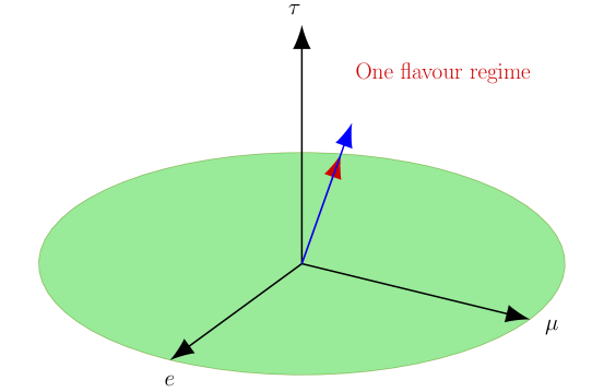
As mentioned
earlier, , therefore and no baryogenesis is possible in this mass regime.
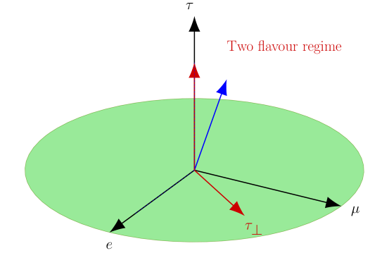
GeV (Two flavour regime): In this regime the flavour is in equilibrium and hence distinguishable but and flavours cannot be distinguished since they are not in equilibrium. It is therefore convenient to define two sets of CP asymmetry parameters and , the index takes the values and (, Fig.1). The Boltzmann equations lead to the two asymmetries and . They are related to and by a flavour coupling A-matrix given by [42]
| (4.47) |
The final baryon asymmetry is then calculated as
| (4.48) |
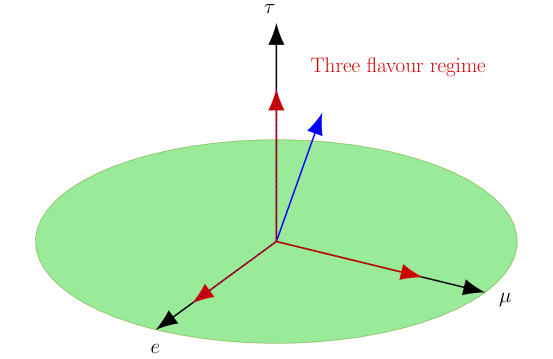
GeV (Three flavour regime): Here muon flavour comes to an equilibrium thus three lepton flavours are separately distinguishable. Now the flavour index can just be or or . In this case the matrix, whose element relates and , is given by[42]
| (4.49) |
Now the final baryon asymmetry normalized to the entropy density, is given by
| (4.50) |
5 Numerical discussion
Before going into detail of the numerical analysis, let us address an important issue first. Unlike the other literatures which also deal with perturbation to the effective light neutrino mass matrix , here we use an exact diagonalization[50] procedure for the effective . This in turn allows us to take large666Here by ‘large’ we mean a number whose square order can not be neglected values of the perturbation parameters (this is not allowed in the perturbative diagonalization procedure). Obviously in our numerical analysis we do not go beyond which implies a full breaking of the leading order symmetry. Here the numerical analysis is basically a two step process in which at first we constrain the primed parameters (e.g. Eq.(3.13) ) by the experimental limits on the neutrino oscillation observables and then explore the related low energy phenomenology.
As it is mentioned earlier that we should carry out the numerical analysis only for the theoretically viable cases, we proceed to constrain the Lagrangian parameters with the experimental bounds on the oscillation data for in (3.7) and in (3.29). Despite the fact that both the mass orderings for the matrix in (3.7) and only the normal mass ordering of in (3.29) are theoretically allowed, given the present global fit oscillation constraints[26], the upper bound 0.17 eV[38] on the sum of the light neutrino masses and non zero values of both the breaking parameters, the latter case is disfavoured along with the inverted ordering for the former. Therefore the detailed discussions on numerical analysis is based entirely on the phenomenological consequences and outcomes for the normal mass ordering case of .
We then turn to the computation of baryogenesis via leptogenesis. Note that the calculation of
the CP asymmetry parameters as well as the other involved decay and scattering process require full information of the Lagrangian
elements, i.e., the parameters of as well as . For this purpose, we first fix the elements of
that correspond to the lowest values of the breaking parameters consistent with the oscillation data.
Then varying the unperturbed values of RH neutrino masses (here the relevant unperturbed parameter is only) we generate
the parameters of using the relation . Thus for the fixed values of the primed parameters
and the corresponding breaking parameters, we are able to calculate for each of the chosen values of unperturbed
RH neutrino masses and hence the elements of . Since has an upper and a lower limit we end up with an upper and a lower
limit on the RH neutrino masses also. Again, a subtle point should be noted that since there are large number values
for consistent with the oscillation data, we are obliged to take the simultaneous minimum values of
the breaking parameters for the computation of baryon asymmetry. However, we also discuss how the large values of the breaking parameters could affect the final asymmetry. A detail numerical discussion is now given in what follows.
5.1 Fit to neutrino oscillation data and predictions on low energy neutrino parameters
For numerical computation, we use the explicit analytic formulae for the light neutrino masses and mixing angles originally obtained in Ref.[50] for a general complex symmetric matrix. Thus after knowing the neutrino mass matrix elements in terms of the model parameters we insert them in to the generalised formula for masses and mixing angles obtained in Ref.[50] (which in priciple enable us to express those oscillation observables in terms of the model parameters) and do a random scanning of the parameters using the experimental constraints on masses and mixing angles. We do not present here the explicit forms of the equations since they are quite lengthy due the complicated structure of the mass matrix as shown in Appendix A.1. In any case, as we said, given the general forms of those equations in Ref.[50], one has just to insert the mass matrix parameters in those equations and do a random scanning of those parameters. In our case, we vary the model parameters within a range , the phase parameter within the interval as and the breaking parameters in the range . Then all the parameters are constrained using the global fit of neutrino data and .
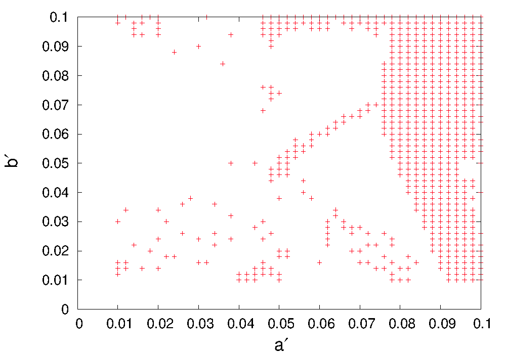
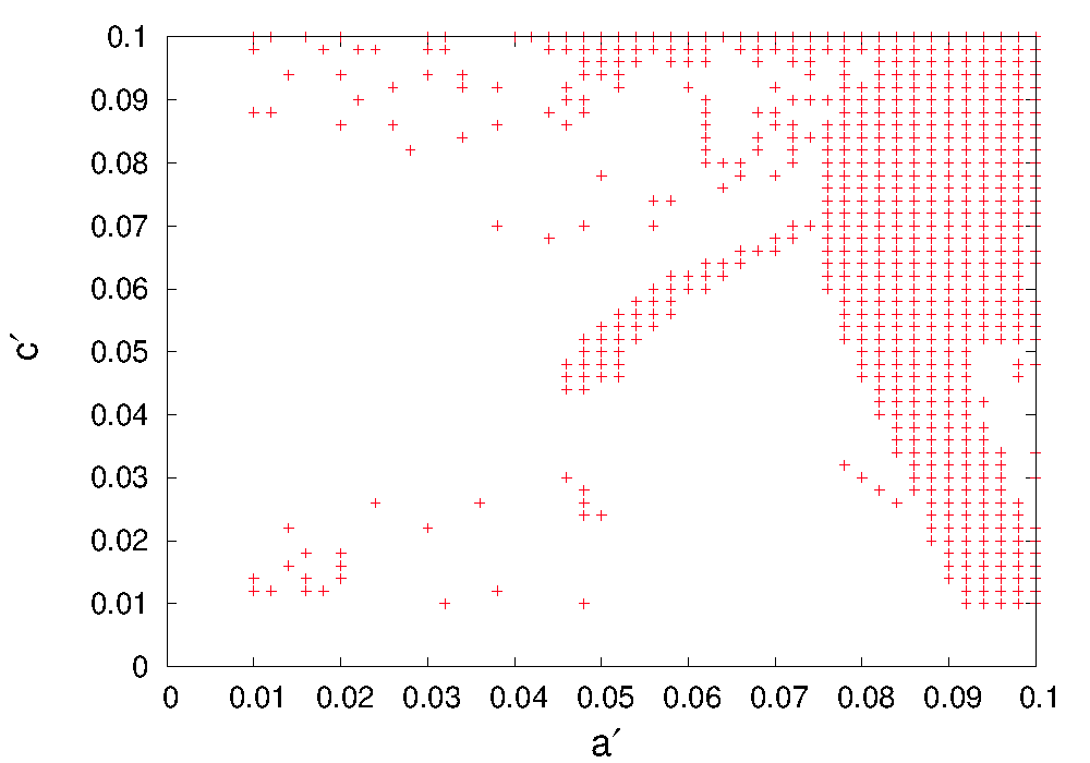
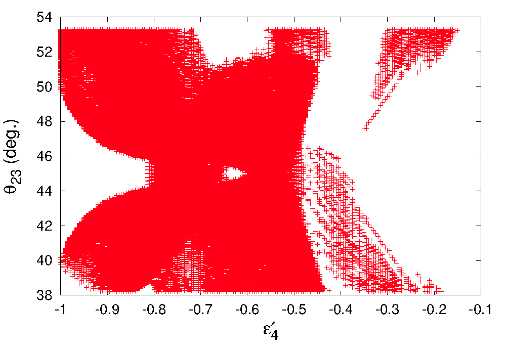
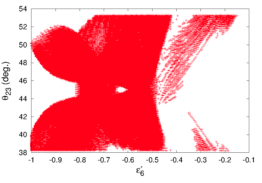
As shown in the upper panel of Fig.2, although and are allowed almost throughout the given range , their all possible combinations in the given range are not allowed777Notice that all the plots in Fig.2 and Fig.3 are two dimensional projections of the six dimensional coupled parameter space allowed by the oscillation data. It is difficult to infer an one to one analytic correlation due to the random shapes of the projections. However, the narrow disallowed strip in Fig.3 could easily be understood, since that corresponds to which means, we essentially have one independent breaking parameter and one can not fit all the oscillation constraints with one breaking parameter in this model.. The phase remains unconstrained, i.e. all possible values in the interval are allowed. The breaking parameters get significant restriction which is depicted in Fig.3. One crucial observation regrading the allowed parameter space should be mentioned here. The constrained parameter space is totally symmetric with respect to the sign of phase , i.e., in other words, if the constrained parameter space contains a certain set of points then the set must belong to the same constrained parameter space. Given the constraints from the neutrino oscillation global fit data, we find it very difficult to fit maximal or near maximal values of with small breaking parameters. For example, to fit to 48∘, one needs and breaking in and for . On the other hand a maximal value of requires and breaking on the same breaking parameters for . However, if we restrict ourselves to consider breaking in one of the parameters up to while keeping the other more than but less than , we can fit the value of between, e.g., (lower panel, Fig.2). For example, the most simultaneous minimal values of and correspond to and breaking in the respective parameters (, ). With this choice of values we can fit to a value .

We have used these minimal values of the breaking parameters in the leptogenesis calculation also. Nevertheless, as one can see, to fit to its maximality or near maximality, this spacial case of TM1 mixing under consideration requires large breaking. On the other hand, a sizeable departure from maximality in the second octant or in the first octant, could be fitted better with relatively small breaking parameters. The matrix also possesses testable prediction on the neutrinoless double beta decay parameter (here ) 3 meV-35 meV. Significant upper limits on are available from ongoing search experiments for decay. KamLAND-Zen [51] and EXO [52] had earlier constrained this value to be eV. Nevertheless, the most impressive upper bound till date is provided by GERDA phase-II data[53]: eV. Though the aforementioned experiments cannot test this model, predictions of our model could be probed by the combined GERDA + MAJORANA experiments [54]. The sensitivity reach of other promising experiments such as LEGEND-200 (40 meV), LEGEND-1K (17 meV) and nEXO (9 meV)[55] are also exciting to probe our predictions. One of the significant result of the matrix is its prediction on the Dirac CP violating phase . Since the symmetry fixes the first column of to the first column of (cf. Eq.2.19), using the equality and the relation in (3.9) one can calculate
| (5.1) |
This is clear from (5.1) that the indicated maximality in the Dirac CP phase from T2K[23] would arise for a maximal atmospheric mixing. One can also track for nonmaximal values of (this has recently been hinted by NOA at 2.6[27]) as shown in the Fig.4.
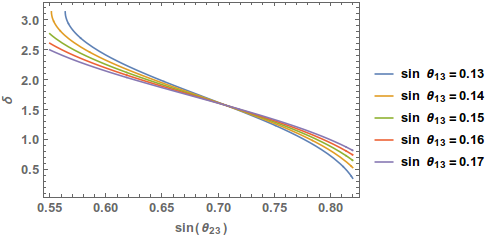
However, please note that, this prediction comes from the residual unbroken symmetry thus this is also present in a pure TM1 mixing. But, as we indicate, in our model, for small values of breaking parameters, it is not possible to reproduce the entire 3 range of . In left panel of Fig.5, we present a probability distribution of allowing one the breaking parameters to vary upto while the other one to . In this case the most probable value of , say is disfavoured at 1.25 by the present best fit of [56]. In the right panel, the distribution for is presented for the most simultaneous minimal values of . Here the most probable value is disfavoured at 1.38. Though the statements on in the global fit is not very precise due to poor statistics, however, future measurements of would be an excellent test of the goodness of the framework under consideration.
5.2 Numerical results for baryogenesis via leptogenesis
Now we turn to the calculations related to baryogenesis via leptogenesis. The main ingredients to evaluate baryon asymmetry are the flavoured CP asymmetry parameters and decay/scattering terms that appear in the relevant Boltzmann equations. Computation of these quantities require explicit values of the unprimed parameters of and the mass scale of . Note that only the primed parameters along with two breaking parameters have been constrained by the oscillation data. Therefore to get the unprimed parameters from the primed ones, we need to vary the mass scale which is a free parameter. Since there are huge number of sets of primed parameters that are consistent with the 3 global fit constraints, it is therefore impractical to numerically solve the BEs for each of the sets. For this, we take a fixed set of primed parameters and vary through a wide range of masses form GeV to GeV to study the phenomena baryogenesis via leptogenesis for each of the mass regimes. Question might arise, which set of the primed parameters should be taken into account for the computation related to baryogenesis? In principle each of the data set for the primed parameters are allowed. Nevertheless, we choose that set of the primed elements which corresponds to the minimum values for the breaking parameters required to fit the oscillation data. In other words, we have readily opted for the minimal symmetry breaking scenario (as already pointed out, the values are and ) to compute the baryon asymmetry in our model. The set of primed parameters are displayed in Table 1.
As explained in the theoretical section, the unflavoured leptogenesis scenario ( GeV) is disfavored for our scheme.
We therefore present our numerical results for the other two regimes in what follows.
-flavoured regime ( GeV GeV): As explained in the previous section, in this regime the flavour is in equilibrium and thus it has a separate identity but and are indistinguishable. So practically here we have two lepton flavours (denoted by 2 or ) and and correspondingly we have CP asymmetry parameters and . In the flavoured Boltzmann equations (4.46), lepton flavour index can take only two values and . Thus we get two equations involving the differentials of flavoured asymmetries and which have to be solved simultaneously (using matrix) to get the values of those asymmetries at very low temperature or equivalently at fairly large value of where these asymmetries get frozen. Those final values of asymmetries are then added up and multiplied by a suitable Sphaleronic conversion factor (cf. (4.48)) to arrive at the observed range of .
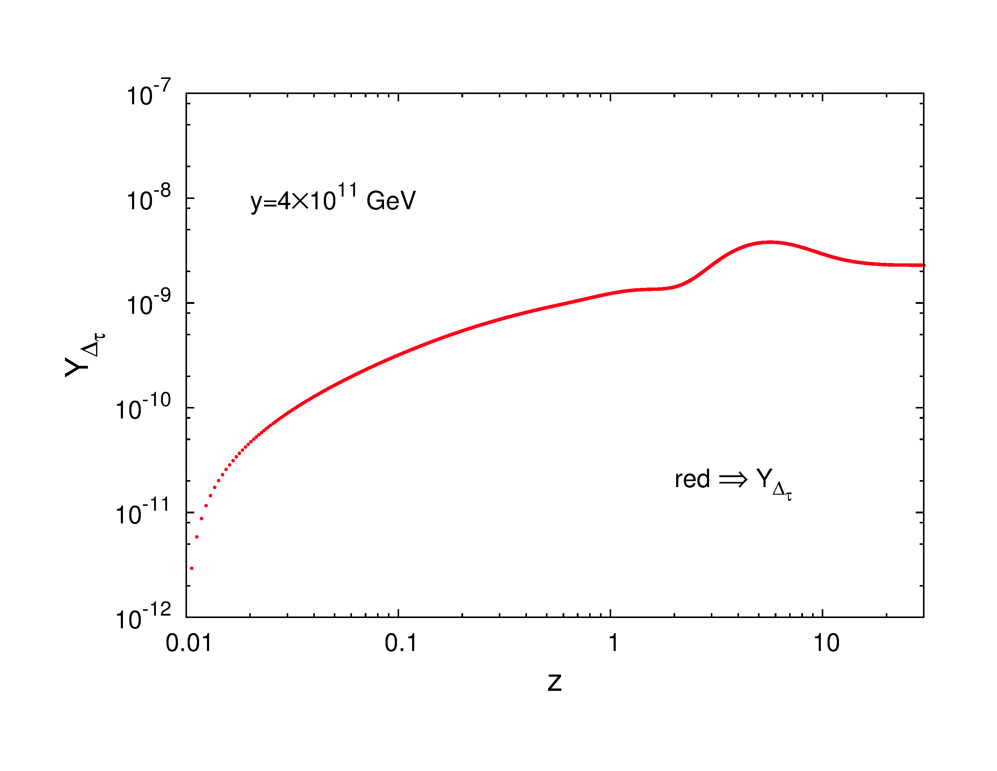
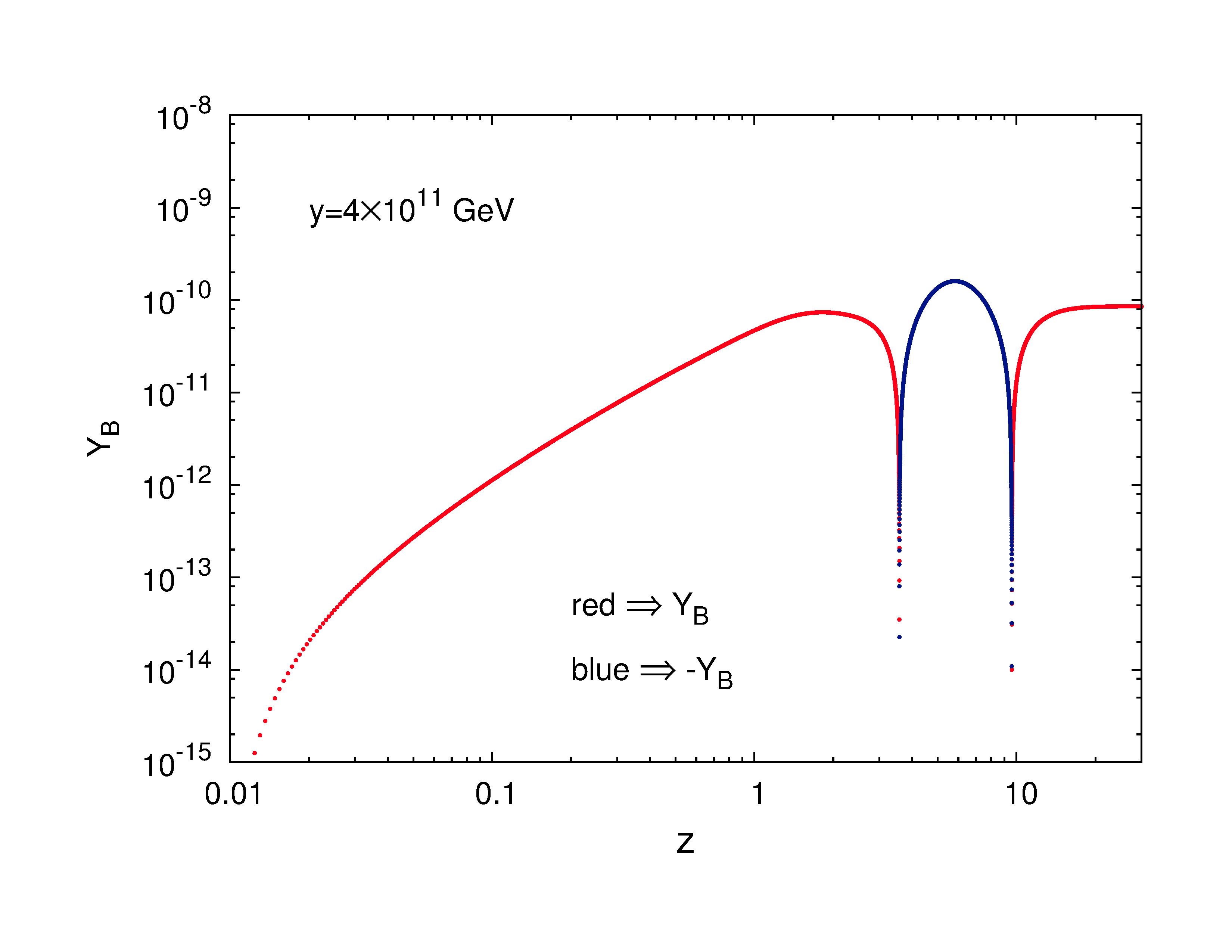
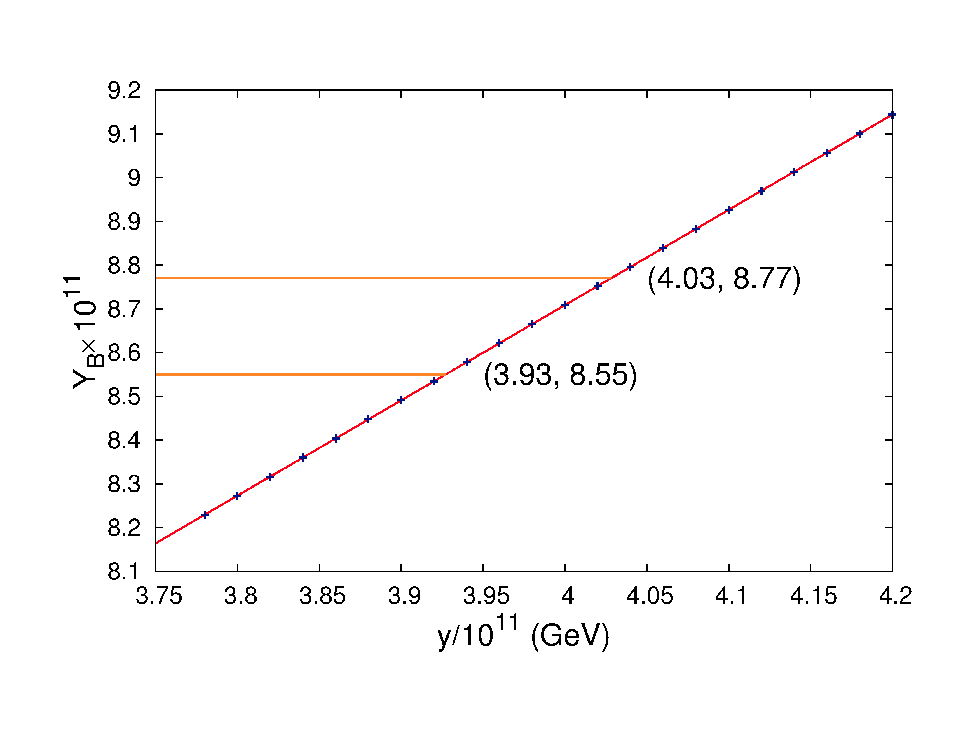
Now for the set of the primed parameters given in Table 1 we generate the unprimed parameters by varying the mass scale parameter over the entire range GeV to GeV. For every value of within this range indeed freezes to a positive value at high , but the correct order of () is achieved when GeV. We present only few such values of and corresponding in the Table 2 for which is mostly within the experimentally observed range .
| (GeV) | ||||||||||
|---|---|---|---|---|---|---|---|---|---|---|
Among all these values we choose GeV and show the variation of asymmetries and finally with
in Fig.6. It can be understood from Table 2 that the value of final baryon asymmetry parameter more or less increases linearly
with the mass scale parameter . Thus it is clear that for the observed range of , we should have a lower and an upper
bound on . The figure in the right side in the lower panel of Fig.6 represents the variation of with .
Two straight lines parallel to the abscissa have been drawn respectively at and
corresponding to the upper and lower bounds on the observed .
The values of where these two straight lines touches the curve give the highest and lowest allowed value for the
mass scale parameter . These values are found to be
GeV and GeV.
Fully flavoured regime ( GeV): In this case all three lepton flavours can be distinguished from one another and consequently there are different CP asymmetry parameters which have to be inserted in suitable places of fully flavour dependent Boltzmann equations (cf. (4.46)). These Boltzmann equations are then solved to obtain the flavoured asymmetry parameters which are required to obtain the final asymmetry parameter . As expected, the CP asymmetry parameters and the final baryon asymmetry parameter are found to be significantly less for the lower masses of right handed neutrinos GeV. So we try with the highest value of the right handed neutrino mass GeV allowed in this regime. With GeV and primed set of parameters as given in Table 1, we calculate CP asymmetry and thereafter solving the full set of coupled Boltzmann equations, we compute . It is found that final value of at high attains a negative value. It has already been made clear in the second paragraph of numerical discussion that we have a similar set of points (Table.1) with every primed parameters unaltered except . Following the discussion of the last paragraph in Sec.4.1, it is easy to understand that the sign of the CP asymmetries will be reversed while they are computed with instead of . Therefore as a result the parameter set of Table.1 with yields a positive value of baryon asymmetry parameter at high , but still it is one order lower than the experimentally observed value of . To be precise, the value of (at ) for is
Few remarks on the effect of the two heavier neutrinos () on the final baryon asymmetry: As already mentioned in Sec.4.1, the resonance enhancement and heavy neutrino flavour oscillation are not significant in our scenario. However, due to the small mass splitting between the RH neutrinos, it is expected that dynamics of the heavy neutrinos are not decoupled since washout due to a particular species of RH neutrino affects the production of the asymmetry due the lighter RH neutrinos, also the asymmetry produced by a heavier one is not fully washed out by the lighter one. This is why we have solved the network of Boltzmann equations where ‘all production’ is affected by ‘all washout’[41]. This could qualitatively be understood by a simple two RH neutrino scenario considering the simplest form of the Boltzmann equations where only the decays and inverse decays are involved (however for a realistic three RH neutrino scenario, where all the other effects, e.g., effects of scattering, charged lepton flavour effect, flavour coupling etc. are involved, the qualitative picture does not change). In this simplest scenario the solution for the lepton asymmetry is given by
| (5.2) |
where is the efficiency of production of lepton asymmetry due to ‘’th RH neutrino. An explicit analytical expression for is given by
| (5.3) |
where ‘’ means the inverse decay and has the standard expression[41] in the hot early universe. If the RH neutrinos are strongly hierarchical, two standard expressions for the efficiency factors are given by[49]
| (5.4) |
where
| (5.5) |
with as an equilibrium neutrino mass eV.
Our task is to show, given our model, whether a numerical integration of (5.3) is consistent with (5.4) or not. If these two equations match, then contribution from the heavier neutrinos are irrelevant, i.e, we are in standard dominated scenario. On the contrary, if they are inconsistent, then we can conclude that contributions from the heavier neutrinos are not negligible.
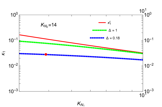
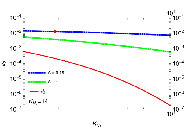
Let us choose the or the ‘2’ flavour for a specific example and denote the decay parameters as and for and respectively. It is clear from the figure on the RHS (top) of Fig.7, that the efficiency factor of the standard dominated scenario and our model do not match at all. In fact, the efficiency factor decreases as we consider smaller breaking of . This is simply due to the fact, that as the breaking parameters which are also related to the mass splitting of the RH neutrinos, become smaller, in addition to the -washout, the washout by also affects the asymmetry production due to decays (In a typical dominated scenario, inverse decay goes out of equilibrium before the decay or inverse decay reaches equilibrium[57]). The blue line represents the for the minimal set of breaking parameters and which corresponds to a mass splitting (cf Eq.4.12) where we allow to vary within the obtained range and take . The red dot represents a particular set () which corresponds to the earlier mentioned simultaneous minimal pair of breaking parameters. The green line corresponds to . As one can see, starting from our scenario which corresponds to small breaking parameters, as one approaches to a pure TM1 mixing which requires complete breaking of the symmetry and hence large breaking parameters, the effect of the next to the lightest of the heavy neutrinos decreases so that the efficiency factor tends to match with its standard expression in a pure dominated or strongly hierarchical case. On the other hand, as one can see from the figure at the bottom in Fig.7, for small values of the breaking parameters, the efficiency factor escapes from the exponential washout (cf. Eq.5.4) due to and increases from its standard value , thus leaves a non-negligible contribution to the final asymmetry.
5.3 Prediction of flux ratios at neutrino telescopes
Recently IceCube [30] has discovered long expected Ultra High Energy (UHE) neutrinos events and thus opened a new era in the neutrino astronomy. IceCube has reported 82 high-energy starting events (HESE) (Including track +shower) which constitute more than 7 excess over the atmospheric background and thus points towards an extraterrestrial origin of the UHE neutrinos (for a latest updated result, please see [58]). Also, no significant spatial clustering has been found[59] and the recent data seems to be consistent with isotropic neutrino flux from uniformly distributed point sources and points towards extra galactic nature of the observed events. Nevertheless, the origin of these UHE neutrinos still remains unknown. Although the HESE events are not consistent888Using a flavour composition 1:1:1 at the earth and deposited energy 60 TeV-10 PeV, 6-years HESE best fit to the spectral index is . However, the 8-years through going muon (TG) data which corresponds to 1000 extraterrestrial neutrinos above 10 TeV, corresponds to a best fit which is close to the theoretically preferred spectrum. with the standard astrophysical ‘one component’ unbroken isotropic power-law spectrum
| (5.6) |
with (much harder spectrum than the HESE best fit) and also suffer constraints from multi-messenger gamma-ray observation[60], ‘two component’ explanation of the observed neutrino flux from purely astrophysical sources is still a plausible scenario [34]. Thus with enhanced statistics at the neutrino telescopes and future determination of the flavour composition of UHE neutrinos at the earth would pin point the viability of the astrophysical sources as the origin of the UHE neutrinos. In our model, without going into any fit to the present data, we predict the the flavour flux ratios at the earth, assuming the conventional and sources. The dominant source of ultra high energy cosmic neutrinos are (hadro-nuclear) collisions in cosmic ray reservoirs such as galaxy clusters and (photo-hadronic) collisions in cosmic ray accelerators such as gamma-ray bursts, active galactic nuclei and blazars[61, 62]. In collisions, protons of TeVPeV range produce neutrinos via the processes and Therefore, the ratio of the normalized flux distributions over flavour is
| (5.7) |
where the superscript denotes ‘source’ and denotes the overall flux normalization. For collisions, one has either leading to the same flux ratios in Eq.5.7 or the resonant production and corresponding normalized flux distributions over flavour
| (5.8) |
In either case, since the Icecube does not distinguish between neutrino and antineutrinos (other than the Glashow resonance: at PeV) we take with as
| (5.9) |
Since the source-to-telescope distance is much greater than the oscillation length, the flavour oscillation probability averaged over many oscillations is given by
| (5.10) |
Thus the flux reaching the telescope is given by
| (5.11) |
which simplifies to
| (5.12) |
where and we have used the unitarity of the PMNS matrix i.e., . With the above background, one can define flavour flux ratios () at the neutrino telescope as
| (5.13) |
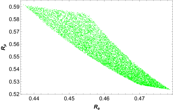
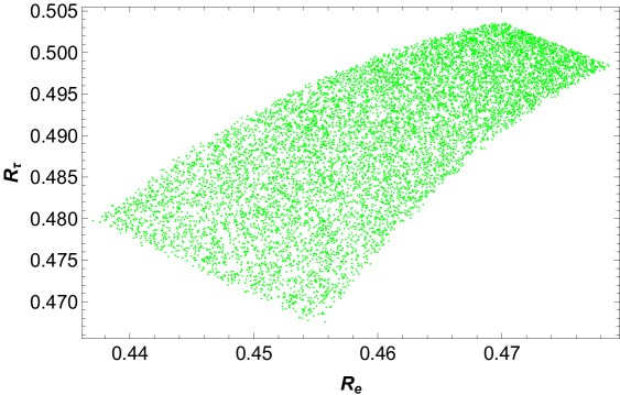
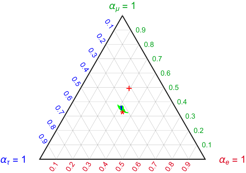
where and is as in (1.4). Note that for the exact TBM, and thus – this is well known[63, 64, 65, 66]. In our model, we find interesting deviation from this democratic flavour distribution at the telescopes. As we show in the Fig. 8 whilst and prefers the values less than the standard value 0.5, prefers values greater than 0.5 in this model. In Fig.9 we present a Ternary plot for a better visualization of the flavour compositions. Here . The red ‘’ represents the TBM democratic prediction 1:1:1. The green area represents the allowed range of the flavours for 3 interval of the mixing parameters. The blue region (within the green one) is our model prediction. The red ‘’ is the HESE best fit 0.29:0.50:0.21[58]. Clearly the present HESE best fit and the flavour composition allowed by standard neutrino oscillation as well as the composition predicted in our model are in tension. Though these could be reconciled well within the HESE CL[58].
5.4 A comparative study with the other works and few final remarks
Though at the end of the introduction section we have tried to focus on the novelty and new results of our work, for the sake of completeness
and a quantitative comparison, we would like to expense few lines in this subsection also. As already pointed out in the introduction,
in a bottom up approach, starting from the residual symmetry framework, we have studied the goodness of the symmetry under the
lamppost of a TM1 symmetry in quite a general way. Though there is sizeable amount work devoted to TBM mixing as we cited in the
introduction, e.g., Ref.[6, 8, 9, 11, 12] etc, most of them discuss either completely broken TBM
or a pure TM1 symmetry. Thus we feel, the results obtained in our work (apart from the correlations which are also present in a pure TM1 mixing)
are entirely novel and more testable. As we have already pointed out, we are motivated by Ref.[24] Ref. [25], where, keeping the TM1
generator unbroken, alteration of the symmetry has been studied. Though the alterations have been done by the usage of the generator
as a CP generator; instead of an exact interchange symmetry. However, here we have studied the modification of the interchange by
breaking it explicitly. Thus, though the philosophy behind our work is same as that of Ref.[24] Ref. [25], phenomenological outcomes are
different due different treatment of the symmetry. Since the underlying philosophy for handling the symmetry is different, our low energy predictions such as the Dirac CP phase as well as the estimated range of are also different from a comprehensive analysis [8] which discusses different variants of TBM mixing. From leptogenesis perspective, our
work and the Ref.[32] share some common ground. To be more precise, the common origin of nonzero and quasi
degeneracy of the RH neutrino masses. However, the analysis is done only with interchange symmetry with one small breaking parameter
(so that the second order terms could be neglected) whereas in our case we have done braking of keeping TM1 symmetry intact and
this in turn leads the structure of the breaking pattern not be arbitrary. In addition, our leptogenesis analysis is rigorous and also include flavour effects
as well as theoretical uncertainties such as flavour couplings. We also show, how starting from our scenario, as one approaches to a pure TM1 mixing,
the effects of the heavy RH neutrinos become weak. We would like to draw the same conclusion for Ref.[33] as we do for Ref.[32].
Though Ref.[9] studied leptogenesis under a TM1 symmetry, the framework is minimal seesaw and thus one of the mass eigenvalue is zero plus
due to the typical structure of the mass matrices, the prediction is and . In addition, the authors assume the RH
masses are arbitrarily close so that resonant condition could be satisfied in a low RH mass scale whereas in our case as we already point out,
one cannot choose the arbitrary mass splitting between the RH neutrinos.
Some final remarks: In this precision era of the low energy neutrino phenomenology, it is a high time for the rigorous computation in any neutrino mass model so that it could be tested in the experiments unambiguously. In this work, we have tried to be as concise as possible in the computation while rigorously studying an unexplored scenario related to the modification to a TBM scheme. We report that, the framework under consideration is not compatible with very small breaking parameters and the neutrino oscillation data. The minimal pair corresponds to and . Even if we allow breaking in both the parameters upto , our work disfavours maximal mixing. Thus in future, strong statements on would be an excellent probe to test the goodness of our idea. In addition, whilst an in-depth computation (with the best of our expertise) of baryogenesis via leptogenesis seeks the RH mass scale to be more than GeV, validity of this framework with relatively small breaking parameters is also testable via its very sharp predictions on the Dirac CP phase as well as UHE neutrino flavour ratios.
6 Conclusion
We have analyzed the broken TBM mass matrices which are invariant under a residual (TBM-Klein) symmetry at the leading order. To explore a predictive scenario, we have opted for the minimal breaking scheme where only is broken to generate a nonzero reactor mixing angle . We started with the Type-I seesaw mechanism which contains the Dirac type and Majorana type as the constituent matrices. In the diagonal basis of the charged lepton as well as the RH neutrino mass matrix , the implemented residual TBM-Klein symmetry leads to degenerate RH neutrino masses. The is then broken in to lift the mass degeneracy as well as to generate nonvanishing value of . Thus the observed small value of restricts the level of degeneracy in the RH neutrino masses. Phenomenologically allowed case in our analysis gives rise to a TM1 type mixing and predicts a normal mass ordering for the light neutrinos. Testable predictions on the Dirac CP phase and the neutrinoless double beta decay parameter have also been obtained. Our analysis is also interesting from leptogenesis perspective. Unlike the standard hierarchical -leptogenesis scenario, here due to the implemented symmetry and the phenomenologically viable breaking pattern of that symmetry, the baryogenesis via leptogenesis scenario is realized due to quasi degenerate RH neutrinos. It has been clarified by a brief mathematical calculation that other two RH neutrinos have sizeable contribution in generating lepton asymmetry. For computation of the final baryon asymmetry we make use of the flavour dependent coupled Boltzmann Equations to track the evolution of the produced lepton asymmetry down to the low temperature scale. Only -flavoured leptogenesis scheme is allowed in our analysis. Consistent with the observed range of a lower and an upper bound on the RH neutrino masses have also been obtained. We also estimate the testable flux ratios of three UHE neutrino flavours (detected at Icecube). At the end we elucidate the novelty and importance of this present work through a comparative study with the existing literature.
Acknowledgement
RS would like to thank Prof. Pasquale Di Bari for a very useful discussion regarding leptogenesis with quasi degenerate neutrinos. RS would like to thank the Royal Society (UK) and SERB (India) for the Newton International Fellowship (NIF). For financial support from Siksha ’O’ Anusandhan (SOA), Deemed to be University, M. C. acknowledges a Post-Doctoral fellowship.
Appendix A Appendix
A.1 Explicit algebraic forms of elements of
Since is symmetric matrix, it has only six independent complex parameters (namely ) each of which contains a common factor in the denominator given by
| (A.1) |
The explicit functional forms of the six independent elements of the are as follows
| (A.2) | |||||
| (A.3) | |||||
| (A.4) | |||||
| (A.5) | |||||
| (A.6) | |||||
| (A.7) | |||||
A.2 Explicit algebraic forms of elements of
The elements of the matrix can be parametrized as
| (A.8) |
where we define the parameters in Eq.(A.8) as
| (A.9) |
with , , ,, being real.
References
- [1] F. P. An et al. [Daya Bay Collaboration], Phys. Rev. Lett. 108, 171803 (2012) [arXiv:1203.1669 [hep-ph]].
- [2] J. K. Ahn et al. [RENO Collaboration], Phys. Rev. Lett. 108, 191802 (2012) [arXiv:1204.0626 [hep-ph]].
- [3] P. F. Harrison, D. H. Perkins and W. G. Scott, Phys. Lett. B 530, 167 (2002) [arXiv:hep-ph/0202074 [hep-ph]]. P. F. Harrison and W. G. Scott, Phys. Lett. B 535, 163 (2002) [arXiv:hep-ph/0203209 [hep-ph]].
- [4] Z. z. Xing, Phys. Lett. B 533, 85 (2002) [arXiv:hep-ph/0204049 [hep-ph]]. X. G. He and A. Zee, Phys. Lett. B 560, 87 (2003) [arXiv:hep-ph/0301092 [hep-ph]]. E. Ma, Phys. Rev. Lett. 90, 221802 (2003) [arXiv:hep-ph/0303126 [hep-ph]].C. I. Low and R. R. Volkas, Phys. Rev. D 68, 033007 (2003) [arXiv:hep-ph/0305243 [hep-ph]]. E. Ma, Phys. Rev. D 70, 031901 (2004) [arXiv:hep-ph/0404199 [hep-ph]]. G. Altarelli and F. Feruglio, Nucl. Phys. B 720, 64 (2005) [arXiv:hep-ph/0504165 [hep-ph]]. S. F. King, JHEP 0508, 105 (2005) [arXiv:hep-ph/0506297 [hep-ph]]. E. Ma, Phys. Rev. D 73, 057304 (2006) [arXiv:hep-ph/0511133 [hep-ph]]. G. Altarelli and F. Feruglio, Nucl. Phys. B 741, 215 (2006) [arXiv:hep-ph/0512103 [hep-ph]]. E. Ma, Mod. Phys. Lett. A 22, 101 (2007) [arXiv:hep-ph/0610342 [hep-ph]]. K. S. Babu and X. G. He, hep-ph/0507217. S. Pakvasa, W. Rodejohann and T. J. Weiler, Phys. Rev. Lett. 100, 111801 (2008) [arXiv:0711.0052 [hep-ph]]. G. Altarelli, F. Feruglio and L. Merlo, JHEP 0905, 020 (2009) [arXiv:0903.1940 [hep-ph]]. E. Ma and D. Wegman, Phys. Rev. Lett. 107, 061803 (2011) [arXiv:1106.4269 [hep-ph]]. R. de Adelhart Toorop, F. Feruglio and C. Hagedorn, Nucl. Phys. B 858, 437 (2012) [arXiv:1112.1340 [hep-ph]]. E. Ma, Phys. Lett. B 583, 157 (2004) [arXiv:hep-ph/0308282 [hep-ph]].
- [5] G. Altarelli and F. Feruglio, Rev. Mod. Phys. 82, 2701 (2010) doi:10.1103/RevModPhys.82.2701 [arXiv:1002.0211 [hep-ph]]. H. Ishimori, T. Kobayashi, H. Ohki, Y. Shimizu, H. Okada and M. Tanimoto, Prog. Theor. Phys. Suppl. 183, 1 (2010) doi:10.1143/PTPS.183.1 [arXiv:1003.3552 [hep-ph]]. S. F. King, Prog. Part. Nucl. Phys. 94, 217 (2017) doi:10.1016/j.ppnp.2017.01.003 [arXiv:1701.04413 [hep-ph]]. S. T. Petcov [arXiv:1711.10806[hep-ph]].
- [6] F. Plentinger and W. Rodejohann, Phys. Lett. B 625, 264 (2005) [arXiv:hep-ph/0507143 [hep-ph]]. X. G. He and A. Zee, Phys. Lett. B 645, 427 (2007) [arXiv:hep-ph/0607163 [hep-ph]]. Z. z. Xing, H. Zhang and S. Zhou, Phys. Lett. B 641, 189 (2006) [arXiv:hep-ph/0607091 [hep-ph]]. R. N. Mohapatra and H. B. Yu, Phys. Lett. B 644, 346 (2007) [arXiv:hep-ph/0610023 [hep-ph]]. M. Hirsch, E. Ma, J. C. Romao, J. W. F. Valle and A. Villanova del Moral, Phys. Rev. D 75, 053006 (2007) [arXiv:hep-ph/0606082 [hep-ph]. K. A. Hochmuth, S. T. Petcov and W. Rodejohann, Phys. Lett. B 654, 177 (2007) [arXiv:0706.2975 [hep-ph]. Y. Koide and H. Nishiura, Phys. Lett. B 669, 24 (2008) [arXiv:0808.0370 [hep-ph]. S. F. King, Phys. Lett. B 659, 244 (2008) [arXiv:0710.0530 [hep-ph]]. C. H. Albright, A. Dueck and W. Rodejohann, Eur. Phys. J. C 70, 1099 (2010) [arXiv:1004.2798 [hep-ph]].X. G. He and A. Zee, Phys. Rev. D 84, 053004 (2011). R. Samanta, M. Chakraborty and A. Ghosal, Nucl. Phys. B 904, 86 (2016) [arXiv:1502.06508 [hep-ph]]. R. Samanta and M. Chakraborty, [arXiv:1703.09579 [hep-ph]].
- [7] B. Adhikary, B. Brahmachari, A. Ghosal, E. Ma and M. K. Parida, Phys. Lett. B 638, 345 (2006). B. Adhikary and A. Ghosal, Phys. Rev. D 78, 073007 (2008) [arXiv:0803.3582 [hep-ph]]. J. Barry and W. Rodejohann, Phys. Rev. D 81, 093002 (2010) Erratum: [Phys. Rev. D 81, 119901 (2010)] [arXiv:1003.2385 [hep-ph]]. Y. F. Li and Q. Y. Liu, Mod. Phys. Lett. A 25, 63 (2010) [arXiv:0911.2670 [hep-ph]]. Y. Lin, Nucl. Phys. B 824, 95 (2010) [arXiv:0905.3534 [hep-ph]]. [arXiv:1106.4359 [hep-ph]]. S. F. King and C. Luhn, JHEP 1203, 036 (2012) [arXiv:1112.1959 [hep-ph]]. W. Rodejohann and H. Zhang, Phys. Rev. D 86, 093008 (2012) [arXiv:1207.1225 [hep-ph]]. S. K. Garg and S. Gupta, JHEP 1310, 128 (2013) [arXiv:1308.3054 [hep-ph]]. V. V. Vien and H. N. Long, Int. J. Mod. Phys. A 28, 1350159 (2013) [arXiv:1312.5034 [hep-ph]]. Z. h. Zhao, JHEP 1411, 143 (2014) doi:10.1007/JHEP11(2014)143 [arXiv:1405.3022 [hep-ph]]. Z. z. Xing and Z. h. Zhao, Rept. Prog. Phys. 79, no. 7, 076201 (2016) [arXiv:1512.04207 [hep-ph]]. J. Talbert, JHEP 1412, 058 (2014) [arXiv:1409.7310 [hep-ph]]. R. Samanta and A. Ghosal, Nucl. Phys. B 911, 846 (2016) [arXiv:1507.02582 [hep-ph]]. J. Zhang and S. Zhou, JHEP 1609, 167 (2016) [arXiv:1606.09591 [hep-ph]]. S. K. Garg, [arXiv:1712.02212 [hep-ph]].
- [8] C. H. Albright and W. Rodejohann, Eur. Phys. J. C 62, 599 (2009) [arXiv:0812.0436 [hep-ph]].
- [9] Z. z. Xing and S. Zhou, Phys. Lett. B 653, 278 (2007) [arXiv:hep-ph/0607302 [hep-ph]].
- [10] W. Grimus and L. Lavoura, JHEP 0809, 106 (2008) [arXiv:0809.0226 [hep-ph]]. W. Grimus and L. Lavoura, Phys. Lett. B 671, 456 (2009) [arXiv:0810.4516 [hep-ph]].
- [11] I. de Medeiros Varzielas and L. Lavoura, J. Phys. G 40, 085002 (2013) [arXiv:1212.3247 [hep-ph]]. Nucl. Phys. B 875, 80 (2013) [arXiv:1306.2358 [hep-ph]]. C. C. Li and G. J. Ding, Nucl. Phys. B 881, 206 (2014) [arXiv:1312.4401 [hep-ph]].
- [12] C. Luhn, S. Nasri and P. Ramond, J. Math. Phys. 48, 073501 (2007) doi:10.1063/1.2734865 [arXiv:hep-th/0701188 [hep-ph]]. J. A. Escobar and C. Luhn, J. Math. Phys. 50, 013524 (2009) [arXiv:0809.0639 [hep-ph]].
- [13] C. S. Lam, Phys. Lett. B 656, 193 (2007) [arXiv:0708.3665 [hep-ph]].
- [14] C. S. Lam, Phys. Rev. Lett. 101, 121602 (2008), [arXiv:0804.2622 [hep-ph]].
- [15] C. S. Lam, Phys. Rev. D 78, 073015 (2008). [arXiv:0809.1185 [hep-ph]].
- [16] D. A. Dicus, S. F. Ge and W. W. Repko, Phys. Rev. D 83, 093007 (2011) [arXiv:1012.2571 [hep-ph]]. S. F. Ge, D. A. Dicus and W. W. Repko, Phys. Lett. B 702, 220 (2011) [arXiv:1104.0602 [hep-ph]]. S. F. Ge, D. A. Dicus and W. W. Repko, Phys. Rev. Lett. 108, 041801 (2012) [arXiv:1108.0964 [hep-ph]]. A. D. Hanlon, S. F. Ge and W. W. Repko, Phys. Lett. B 729, 185 (2014) doi:10.1016/j.physletb.2013.12.063 [arXiv:1308.6522 [hep-ph]].
- [17] H. J. He and F. R. Yin, Phys. Rev. D 84, 033009 (2011) [arXiv:1104.2654 [hep-ph]]. H. J. He and X. J. Xu, Phys. Rev. D 86, 111301 (2012) doi:10.1103/PhysRevD.86.111301 [arXiv:1203.2908 [hep-ph]].
- [18] R.N Mohapatra and S. Nussinov, Phys. Rev. D60(1999)013002. T. Fukuyama and H. Nishiura, [arXiv:hep-ph/9702253 [hep-ph]]. C. S. Lam, Phys. Lett. B 507, 214 (2001) [arXiv:0104116 [hep-ph]]. E. Ma and M. Raidal, Phys. Rev. Lett. 87, 011802 (2001) Erratum: [Phys. Rev. Lett. 87, 159901 (2001)] [arXiv:0102255 [hep-ph]]. K. R. S. Balaji, W. Grimus and T. Schwetz, Phys. Lett. B 508, 301 (2001) [arXiv:0104035 [hep-ph]]. A. Ghosal, [arXiv:hep-ph/0304090. [hep-ph]]. A. Ghosal, Mod. Phys. Lett. A 19, 2579 (2004). J. C. Gomez-Izquierdo and A. Perez-Lorenzana, Phys. Rev. D 77, 113015 (2008) [arXiv:0711.0045 [hep-ph]]. J. C. Gomez-Izquierdo and A. Perez-Lorenzana, Phys. Rev. D 82, 033008 (2010) [arXiv:0912.5210 [hep-ph]]. J. C. Gómez-Izquierdo, F. Gonzalez-Canales and M. Mondragón, Int. J. Mod. Phys. A 32, no. 28-29, 1750171 (2017) [arXiv:1705.06324 [hep-ph]]. Z. z. Xing and Z. h. Zhao, Rept. Prog. Phys. 79, no. 7, 076201 (2016) [arXiv:1512.04207 [hep-ph]].
- [19] R. Samanta, P. Roy and A. Ghosal, Eur. Phys. J. C 76, no. 12, 662 (2016) [arXiv:1604.06731 [hep-ph]]. R. Samanta, P. Roy and A. Ghosal, Acta Phys. Polon. Supp. 9, 807 (2016) [arXiv:1604.01206 [hep-ph]]. R. Samanta, M. Chakraborty, P. Roy and A. Ghosal, JCAP 1703, no. 03, 025 (2017) doi:10.1088/1475-7516/2017/03/025 [arXiv:1610.10081 [hep-ph]]. R. Sinha, R. Samanta and A. Ghosal, JHEP 1712, 030 (2017) [arXiv:1706.00946 [hep-ph]]
- [20] P. F. Harrison and W. G. Scott, Phys. Lett. B 547, 219 (2002) [arXiv:0210197 [hep-ph]]. W. Grimus and L. Lavoura, Phys. Lett. B 579, 113 (2004) [arXiv:0305309 [hep-ph]]. Fortsch. Phys. 61, 535 (2013) [arXiv:1207.1678 [hep-ph]]. R. N. Mohapatra and C. C. Nishi, JHEP 1508, 092 (2015) [arXiv:1506.06788 [hep-ph]]. Also see: G. Ecker, W. Grimus, H. Neufeld, J.Phys. A20, L807 (1987); Int.J.Mod.Phys. A3, 603 (1988). W. Grimus and M. N. Rebelo, Phys. Rept. 281, 239 (1997) [arXiv:9506272 [hep-ph]].
- [21] E. Ma, Phys. Lett. B 752, 198 (2016) [arXiv:1510.02501 [hep-ph]].
- [22] R. N. Mohapatra and C. C. Nishi, Phys. Rev. D 86, 073007 (2012) doi:10.1103/PhysRevD.86.073007 [arXiv:1208.2875 [hep-ph]]. F. Feruglio, C. Hagedorn and R. Ziegler, JHEP 1307, 027 (2013) [arXiv:1211.5560 [hep-ph]]. M. Holthausen, M. Lindner and M. A. Schmidt, JHEP 1304, 122 (2013) [arXiv:1211.6953 [hep-ph]]. M. C. Chen, M. Fallbacher, K. T. Mahanthappa, M. Ratz and A. Trautner, Nucl. Phys. B 883, 267 (2014) [arXiv:1402.0507 [hep-ph]]. G. J. Ding, S. F. King, C. Luhn and A. J. Stuart, JHEP 1305, 084 (2013) [arXiv:1303.6180 [hep-ph]]. G. J. Ding, S. F. King and A. J. Stuart, JHEP 1312, 006 (2013) [arXiv:1307.4212 [hep-ph]]. F. Feruglio, C. Hagedorn and R. Ziegler, Eur. Phys. J. C 74, 2753 (2014) doi:10.1140/epjc/s10052-014-2753-2 [arXiv:1303.7178 [hep-ph]]. P. Chen, C. Y. Yao and G. J. Ding, Phys. Rev. D 92, no. 7, 073002 (2015) [arXiv:1507.03419 [hep-ph]]. H. J. He, W. Rodejohann and X. J. Xu, Phys. Lett. B 751, 586 (2015) [arXiv:1507.03541 [hep-ph]]. C. C. Nishi, Phys. Rev. D 93, no. 9, 093009 (2016) [arXiv:1601.00977 [hep-ph]]. C. C. Nishi and B. L. Sánchez-Vega, JHEP 1701, 068 (2017) [arXiv:1611.08282 [hep-ph]]. J. T. Penedo, S. T. Petcov and A. V. Titov, JHEP 1712, 022 (2017) [arXiv:1705.00309 [hep-ph]]. R. Samanta, P. Roy and A. Ghosal, [arXiv:1712.06555 [hep-ph]]. N. Nath, Z. z. Xing and J. Zhang, [arXiv:1801.09931 [hep-ph]]. A comprehensive review : S. F. King, Prog. Part. Nucl. Phys. 94, 217 (2017) [arXiv:1701.04413 [hep-ph]].
- [23] K. Abe et al. [T2K Collaboration], Phys. Rev. Lett. 118, no. 15, 151801 (2017) [arXiv:1701.00432[hep-ex]].
- [24] S. Gupta, A. S. Joshipura and K. M. Patel, Phys. Rev. D 85, 031903 (2012) [arXiv:1112.6113 [hep-ph]].
- [25] W. Rodejohann and X. J. Xu, Phys. Rev. D 96, no. 5, 055039 (2017) [arXiv:1705.02027 [hep-ph]].
- [26] F. Capozzi, E. Di Valentino, E. Lisi, A. Marrone, A. Melchiorri and A. Palazzo, Phys. Rev. D 95, no. 9, 096014 (2017) doi:10.1103/PhysRevD.95.096014 [arXiv:1703.04471 [hep-ph]].
- [27] P. Adamson et al. [NOvA Collaboration], Phys. Rev. Lett. 118, no. 15, 151802 (2017) doi:10.1103/PhysRevLett.118.151802 [arXiv:1701.05891 [hep-ph]].
- [28] K. A. Olive et al. [Particle Data Group], Chin. Phys. C 38, 090001 (2014).
- [29] A. D. Sakharov, Pisma Zh. Eksp. Teor. Fiz. 5, 32 (1967) [JETP Lett. 5, 24 (1967)] [Sov. Phys. Usp. 34, 392 (1991)] [Usp. Fiz. Nauk 161, 61 (1991)].
- [30] M. G. Aartsen et al. [IceCube Collaboration], Phys. Rev. Lett. 111, 021103 (2013) doi:10.1103/PhysRevLett.111.021103 [arXiv:1304.5356 [astro-ph.HE]]. M. G. Aartsen et al. [IceCube Collaboration], Science 342, 1242856 (2013) doi:10.1126/science.1242856 [arXiv:1311.5238 [astro-ph.HE]]. M. G. Aartsen et al. [IceCube Collaboration], Phys. Rev. Lett. 113, 101101 (2014) doi:10.1103/PhysRevLett.113.101101 [arXiv:1405.5303 [astro-ph.HE]]. M. G. Aartsen et al. [IceCube Collaboration], arXiv:1510.05223 [astro-ph.HE]. M. G. Aartsen et al. [IceCube Collaboration], arXiv:1710.01191 [astro-ph.HE].
- [31] M. G. Aartsen et al. [IceCube Collaboration], Astrophys. J. 835, no. 2, 151 (2017) doi:10.3847/1538-4357/835/2/151 [arXiv:1609.04981 [astro-ph.HE]]. arXiv:1710.01179 [astro-ph.HE].
- [32] R. N. Mohapatra and S. Nasri, Phys. Rev. D 71, 033001 (2005) doi:10.1103/PhysRevD.71.033001 [hep-ph/0410369]. R. N. Mohapatra, S. Nasri and H. B. Yu, Phys. Lett. B 615, 231 (2005) doi:10.1016/j.physletb.2005.03.082 [hep-ph/0502026].
- [33] S. F. Ge, H. J. He and F. R. Yin, JCAP 1005, 017 (2010) [arXiv:1001.0940 [hep-ph]].
- [34] Y. Sui and P. S. Bhupal Dev, JCAP 1807, no. 07, 020 (2018) doi:10.1088/1475-7516/2018/07/020 [arXiv:1804.04919 [hep-ph]].
- [35] F. P. An et al. [Daya Bay Collaboration], Phys. Rev. Lett. 115, no. 11, 111802 (2015) [arXiv:1505.03456 [hep-ph]].
- [36] B. Karmakar and A. Sil, Phys. Rev. D 91, 013004 (2015) [arXiv:1407.5826 [hep-ph]].
- [37] P. A. R. Ade et al. [Planck Collaboration], Astron. Astrophys. 571, A16 (2014) doi:10.1051/0004-6361/201321591 [arXiv:arXiv:1303.5076 [astro-ph.CO]].
- [38] P. A. R. Ade et al. [Planck Collaboration], Astron. Astrophys. 594, A13 (2016) doi:10.1051/0004-6361/201525830 [arXiv:1502.01589[astro-ph.CO]]. N. Aghanim et al. [Planck Collaboration], Astron. Astrophys. 596, A107 (2016) doi:10.1051/0004-6361/201628890 arXiv:arXiv:1605.02985 [astro-ph.CO]].
- [39] M. Fukugita and T. Yanagida, Phys. Lett. B 174, 45 (1986). A. Riotto and M. Trodden, Ann. Rev. Nucl. Part. Sci. 49, 35 (1999) [arXiv:hep-ph/9901362]. S. Davidson, E. Nardi and Y. Nir, Phys. Rept. 466, 105 (2008) doi:10.1016/j.physrep.2008.06.002 [arXiv:0802.2962 [hep-ph]].
- [40] E. W. Kolb and M. S. Turner, Front. Phys. 69, 1 (1990).
- [41] A. Pilaftsis and T. E. J. Underwood, Nucl. Phys. B 692, 303 (2004) [arXiv:hep-ph/0309342 ].
- [42] A. Abada, S. Davidson, A. Ibarra, F.-X. Josse-Michaux, M. Losada and A. Riotto, JHEP 0609, 010 (2006) [arXiv:hep-ph/0605281]. E. Nardi, Y. Nir, E. Roulet and J. Racker, JHEP 0601, 164 (2006) [hep-ph/0601084]. P. S. B. Dev, P. Di Bari, B. Garbrecht, S. Lavignac, P. Millington and D. Teresi, [arXiv:1711.02861 [hep-ph]].
- [43] P. S. Bhupal Dev, P. Millington, A. Pilaftsis and D. Teresi, Nucl. Phys. B 886, 569 (2014) doi:10.1016/j.nuclphysb.2014.06.020 [arXiv:1404.1003 [hep-ph]].
- [44] B. Dev, M. Garny, J. Klaric, P. Millington and D. Teresi, Int. J. Mod. Phys. A 33, 1842003 (2018) doi:10.1142/S0217751X18420034 [arXiv:1711.02863 [hep-ph]].
- [45] W. Buchmuller, P. Di Bari and M. Plumacher, Nucl. Phys. B 665, 445 (2003) [arXiv:hep-ph/0302092 [hep-ph]].
- [46] J. Edsjo and P. Gondolo, Phys. Rev. D 56, 1879 (1997) [arXiv:hep-ph/9704361].
- [47] B. Adhikary, M. Chakraborty and A. Ghosal, Phys. Rev. D 93, no. 11, 113001 (2016) [arXiv:1407.6173 [hep-ph]]. R. Samanta, M. Chakraborty, P. Roy and A. Ghosal, JCAP 1703, no. 03, 025 (2017) [arXiv:1610.10081 [hep-ph]].
- [48] B. Dev, M. Garny, J. Klaric, P. Millington and D. Teresi, [arXiv:1711.02863[hep-ph]].
- [49] W. Buchmuller, P. Di Bari and M. Plumacher, Annals Phys. 315, 305 (2005) [arXiv:hep-ph/0401240].
- [50] B. Adhikary, M. Chakraborty and A. Ghosal, JHEP 1310, 043 (2013) Erratum: [JHEP 1409, 180 (2014)] [arXiv:1307.0988 [hep-ph]].
- [51] K. Asakura et al. [KamLAND-Zen Collaboration], Nucl. Phys. A 946, 171 (2016) [arXiv:1509.03724 [hep-ph]].
- [52] M. Auger et al. [EXO-200 Collaboration], Phys. Rev. Lett. 109, 032505 (2012) [arXiv:1205.5608 [hep-ph]].
- [53] B. Majorovits [GERDA Collaboration], AIP Conf. Proc. 1672, 110003 (2015) [arXiv:1506.00415 [hep-ph]].
- [54] N. Abgrall et al. [Majorana Collaboration], Adv. High Energy Phys. 2014, 365432 (2014) [arXiv:1308.1633 [hep-ph]].
- [55] M. Agostini, G. Benato and J. Detwiler, Phys. Rev. D 96, no. 5, 053001 (2017) [arXiv:1705.02996 [hep-ph]].
- [56] http://www.nu-fit.org/?q=node/166
- [57] S. Blanchet and P. Di Bari, JCAP 0606, 023 (2006) doi:10.1088/1475-7516/2006/06/023 [hep-ph/0603107].
- [58] http://npc.fnal.gov/wp-content/uploads/2018/09/180830_fermilab2.pdf.
- [59] S. Adrian-Martinez et al. [ANTARES and IceCube Collaborations], Astrophys. J. 823, no. 1, 65 (2016) doi:10.3847/0004-637X/823/1/65 [arXiv:1511.02149 [hep-ex]].
- [60] J. K. Becker, Phys. Rept. 458, 173 (2008) doi:10.1016/j.physrep.2007.10.006 [arXiv:0710.1557 [astro-ph]].
- [61] M. Ahlers and F. Halzen, Rept. Prog. Phys. 78, no. 12, 126901 (2015). doi:10.1088/0034-4885/78/12/126901
- [62] S. Hummer, M. Ruger, F. Spanier and W. Winter, Astrophys. J. 721, 630 (2010) doi:10.1088/0004-637X/721/1/630 [arXiv:1002.1310 [astro-ph.HE]].
- [63] J. G. Learned and S. Pakvasa, Astropart. Phys. 3, 267 (1995) doi:10.1016/0927-6505(94)00043-3 [hep-ph/9405296, hep-ph/9408296].
- [64] S. Pakvasa, W. Rodejohann and T. J. Weiler, JHEP 0802, 005 (2008) doi:10.1088/1126-6708/2008/02/005 [arXiv:0711.4517 [hep-ph]].
- [65] W. Rodejohann, JCAP 0701, 029 (2007) doi:10.1088/1475-7516/2007/01/029 [hep-ph/0612047].
- [66] Z. z. Xing and S. Zhou, Phys. Lett. B 666, 166 (2008) doi:10.1016/j.physletb.2008.07.011 [arXiv:0804.3512 [hep-ph]].