A thread-parallel algorithm for anisotropic mesh adaptation
Abstract
Anisotropic mesh adaptation is a powerful way to directly minimise the computational cost of mesh based simulation. It is particularly important for multi-scale problems where the required number of floating-point operations can be reduced by orders of magnitude relative to more traditional static mesh approaches.
Increasingly, finite element and finite volume codes are being optimised for modern multi-core architectures. Typically, decomposition methods implemented through the Message Passing Interface (MPI) are applied for inter-node parallelisation, while a threaded programming model, such as OpenMP, is used for intra-node parallelisation. Inter-node parallelism for mesh adaptivity has been successfully implemented by a number of groups. However, thread-level parallelism is significantly more challenging because the underlying data structures are extensively modified during mesh adaptation and a greater degree of parallelism must be realised.
In this paper we describe a new thread-parallel algorithm for anisotropic mesh adaptation algorithms. For each of the mesh optimisation phases (refinement, coarsening, swapping and smoothing) we describe how independent sets of tasks are defined. We show how a deferred updates strategy can be used to update the mesh data structures in parallel and without data contention. We show that despite the complex nature of mesh adaptation and inherent load imbalances in the mesh adaptivity, a parallel efficiency of 60% is achieved on an 8 core Intel Xeon Sandybridge, and a 40% parallel efficiency is achieved using 16 cores in a 2 socket Intel Xeon Sandybridge ccNUMA system.
keywords:
anisotropic mesh adaptation, finite element analysis, multi-core, OpenMP1 Introduction
Resolution in time and space are often the limiting factors in achieving accurate simulations for real world problems across a wide range of applications in science and engineering. The brute force strategy is typical, whereby resolution is increased throughout the domain until the required accuracy is achieved. This is successful up to a point when a numerical method is relatively straightforward to scale up on parallel computers, for example finite difference or lattice Boltzmann methods. However, this also leads to a large increase in the computational requirements. In practice, this means simulation accuracy is usually determined by the available computational resources and an acceptable time to solution rather than the actual needs of the problem.
Finite element and finite volume methods on unstructured meshes offer significant advantages for many real world applications. For example, meshes comprised of simplexes that conform to complex geometrical boundaries can now be generated with relative ease. In addition, simplexes are well suited to varying the resolution of the mesh throughout the domain, allowing for local coarsening and refinement of the mesh without hanging nodes. It is common for these codes to be memory bound because of the indirect addressing and the subsequent irregular memory access patterns that the unstructured data structures introduce. However, discontinuous Galerkin and high order finite element methods are becoming increasingly popular because of their numerical properties and associated compact data structure allows data to be easily streamed on multi-core architectures.
A difficulty with mesh based modelling is that the mesh is generated before the solution is known, however, the local error in the solution is related to the local mesh resolution. The practical consequence of this is that a user may have to vary the resolution at the mesh generation phase and rerun simulation several times before a satisfactory result is achieved. However, this approach is inefficient, often lacks rigour and may be completely impractical for multiscale time-dependent problems where superfluous computation may well be the dominant cost of the simulation.
Anisotropic mesh adaptation methods provide an important means to minimise superfluous computation associated with over resolving the solution while still achieving the required accuracy, e.g. [buscaglia1997anisotropic, agouzal1999adaptive, pain_tetrahedral_2001, li20053d]. In order to use mesh adaptation within a simulation, the application code requires a method to estimate the local solution error. Given an error estimate it is then possible to calculate the required local mesh resolution in order to achieve a specific solution accuracy.
There are a number of examples where this class of adaptive mesh methods has been extended to distributed memory parallel computers. The main challenge in performing mesh adaptation in parallel is maintaining a consistent mesh across domain boundaries. One approach is to first lock the regions of the mesh which are shared between processes and for each process to apply the serial mesh adaptation operation to the rest of the local domain. The domain boundaries are then perturbed away from the locked region and the lock-adapt iteration is repeated [coupez2000parallel]. Freitag et al. [freitag1995cient, Freitag98thescalability] considered a fine grained approach whereby a global task graph is defined which captures the data dependencies for a particular mesh adaptation kernel. This graph is coloured in order to identify independent sets of operations. The parallel algorithm then progresses by selecting an independent set (vertices of the same colour) and applying mesh adaptation kernels to each element of the set. Once a sweep through a set has been completed, data is synchronised between processes, and a new independent set is selected for processing. In the approach described by Alauzet et al. [alauzet2006parallel], each process applies the serial adaptive algorithm, however rather than locking the halo region, operations to be performed on the halo are first stashed in buffers and then communicated so that the same operations will be performed by all processes that share mesh information. For example, when coarsening is applied all the vertices to be removed are computed. All operations which are local are then performed while pending operations in the shared region are exchanged. Finally, the pending operations in the shared region are applied.
However, over the past decade there has been a trend towards multi-core compute nodes. Indeed, it is assumed that the compute nodes of a future exascale supercomputer will each contain thousands or even tens of thousands of cores [dongarra2011exascale]. On multi-core architectures, a popular parallel programming paradigm is to use thread-based parallelism, such as OpenMP, to exploit shared memory within a shared memory node and a message passing using MPI for interprocess communication. When the computational intensity is sufficiently high, a third level of parallelisation may be implemented via SIMD instructions at the core level. There are some opportunities to improve performance and scalability by reducing communication needs, memory consumption, resource sharing as well as improved load balancing [rabenseifner2009hybrid]. However, the algorithms themselves must also have a high degree of thread parallelism if they are to have a future on multi-core architectures; whether it be CPU or coprocessor based.
In this paper we take a fresh look at the anisotropic adaptive mesh methods in 2D to develop new scalable thread-parallel algorithms suitable for modern multi-core architectures. We show that despite the irregular data access patterns, irregular workload and need to rewrite the mesh data structures; good parallel efficiency can be achieved. The key contributions are:
-
1.
The first threaded implementation of anisotropic mesh adaptation.
-
2.
Demonstration of parallel efficiencies of 60% on 8 core UMA architecture and 40% on 16 core ccNUMA architecture.
-
3.
Algorithms for selection of maximal independent sets for each sweep of mesh optimisation.
-
4.
Use of deferred update to avoid data contention and to parallelise updates to mesh data structures.
The algorithms described in this paper have been implemented in the open source code PRAgMaTIc (Parallel anisotRopic Adaptive Mesh ToolkIt)111https://launchpad.net/pragmatic. PRAgMaTIc also includes MPI parallelisation, which, for space reasons, will be covered in a forthcoming paper. The remainder of the paper is laid out as follows: §2 gives an overview of the anisotropic adaptive mesh procedure; §3 describes the thread-parallel algorithm; and §4 illustrates how well the algorithm scales for a benchmark problem. We conclude with a discussion on future work and possible implications of this work.
2 Overview
In this section we will give an overview of anisotropic mesh adaptation. In particular, we focus on the element quality as defined by an error metric and the anisotropic adaptation kernels which iteratively improve the local mesh quality as measured by the worst local element.
2.1 Error control
Solution discretisation errors are closely related to the size and the shape of the elements. However, in general meshes are generated using a priori information about the problem under consideration when the solution error estimates are not yet available. This may be problematic because:
-
1.
Solution errors may be unacceptably high.
-
2.
Parts of the solution may be over-resolved, thereby incurring unnecessary computational expense.
A solution to this is to compute appropriate local error estimates, and use this information to compute a field on the mesh which specifies the local mesh resolution requirement. In the most general case this is a metric tensor field so that the resolution requirements can be specified anisotropically; for a review of the procedure see [frey2005anisotropic]. Size gradation control can be applied to this metric tensor field to ensure that there are not abrupt changes in element size [alauzet2010size].
2.2 Element quality
As discretisation errors are dependent upon element shape as well as size, a number of different measures of element quality have been proposed, e.g. [buscaglia1997anisotropic, vasilevskii1999adaptive, agouzal1999adaptive, tam2000anisotropic, pain_tetrahedral_2001]. For the work described here, we use the element quality measure for triangles proposed by Vasilevskii et al. [vasilevskii1999adaptive]:
| (1) |
where is the area of element and is its perimeter as measured with respect to the metric tensor as evaluated at the element’s centre. The first factor () is used to control the shape of element . For an equilateral triangle with sides of length in metric space, and ; and so . For non-equilateral triangles, . The second factor () controls the size of element . The function is smooth and defined as:
| (2) |
which has a single maximum of unity with and decreases smoothly away from this with . Therefore, when the sum of the lengths of the edges of is equal to , e.g. an equilateral triangle with sides of unit length, and otherwise. Hence, taken together, the two factors in (1) yield a maximum value of unity for an equilateral triangle with edges of unit length, and decreases smoothly to zero as the element becomes less ideal.
2.3 Overall adaptation procedure
The mesh is adapted through a series of local operations: edge collapse (§2.4.1); edge refinement (§2.4.2); element-edge swaps (§2.4.3); and vertex smoothing (§2.4.4). While the first two of these operations control the local resolution, the latter two operations are used to improve the element quality.
Algorithm 1 gives a high level view of the anisotropic mesh adaptation procedure as described by [li20053d]. The inputs are , the piecewise linear mesh from the modelling software, and , the node-wise metric tensor field which specifies anisotropically the local mesh resolution requirements. Coarsening is initially applied to reduce the subsequent computational and communication overheads. The second stage involves the iterative application of refinement, coarsening and mesh swapping to optimise the resolution and the quality of the mesh. The algorithm terminates once the mesh optimisation algorithm converges or after a maximum number of iterations has been reached. Finally, mesh quality is fine-tuned using some vertex smoothing algorithm (e.g. quality-constrained Laplacian smoothing [freitag1996comparisonw], optimisation-based smoothing [freitag1995cient]), which aims primarily at improving worst-element quality.
2.4 Adaptation kernels
2.4.1 Coarsening
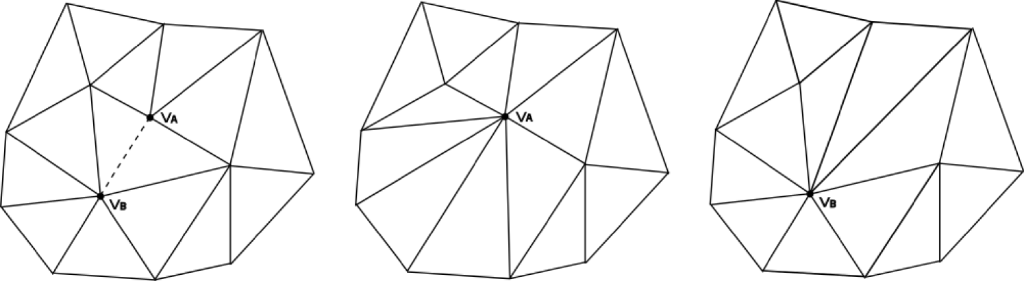
Coarsening is the process of lowering mesh resolution locally by removing mesh elements, leading to a reduction in the computational cost. Here this is done by collapsing an edge to a single vertex, thereby removing all elements that contain this edge. An example of this operation is shown in Figure 1.
2.4.2 Refinement
Refinement is the process of increasing mesh resolution locally. It encompasses two operations: splitting of edges; and subsequent division of elements. When an edge is longer than desired, it is bisected. An element can be split in three different ways, depending on how many of its edges are bisected:
-
1.
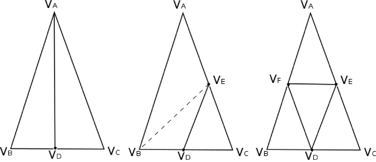
When only one edge is marked for refinement, the element can be split across the line connecting the mid-point of the marked edge and the opposite vertex. This operation is called bisection and an example of it can be seen on the left side of Figure 2 (left shape).
-
2.
When two edges are marked for refinement, the element is divided into three new elements. This case is shown in Figure 2 (middle shape). The parent element is split by creating a new edge connecting the mid-points of the two marked edges. This leads to a newly created triangle and a non-conforming quadrilateral. The quadrilateral can be split into two conforming triangles by dividing it across one of its diagonals, whichever is shorter.
-
3.
When all three edges are marked for refinement, the element is divided into four new elements by connecting the mid-points of its edges with each other. This operation is called regular refinement and an example of it can be seen in Figure 2 (right shape).
2.4.3 Swapping
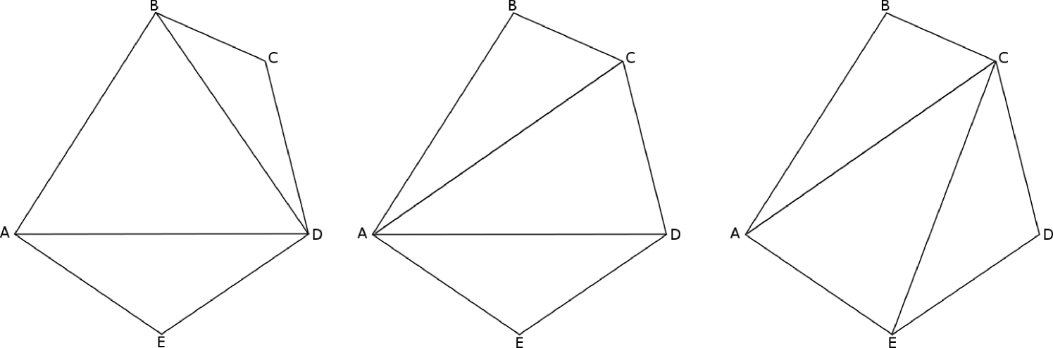
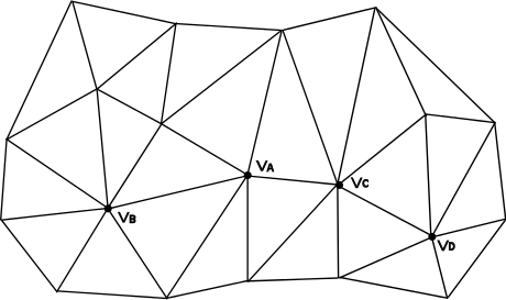
In 2D, swapping is done in the form of edge flipping, i.e. flipping an edge shared by two elements, e.g. Figure 3. The operation considers the quality of the swapped elements - if the minimum element quality has improved then the original mesh triangles are replaced with the edge swapped elements.
Whereas in refinement, propagation is necessary in order to eliminate nonconformities, swapping operations may also propagate because topological changes might give rise to new configurations of better quality. An illustration of this is shown in Figure 4. After an edge has been flipped, the local topology is modified and adjacent edges which were not considered for flipping before are now candidates. This procedure results in a Delaunay triangulation, i.e. one in which the minimum element angle in the mesh is the largest possible one with respect to all other triangulations of the mesh [KulkarniBCP09].
2.4.4 Quality constrained Laplacian Smooth
The kernel of the vertex smoothing algorithm should relocate the central vertex such that the local mesh quality is increased (see Figure 5). Probably the best known heuristic for mesh smoothing is Laplacian smoothing, first proposed by Field [field_laplacian_1988]. This method operates by moving a vertex to the barycentre of the set of vertices connected by a mesh edge to the vertex being repositioned. The same approach can be implemented for non-Euclidean spaces; in that case all measurements of length and angle are performed with respect to a metric tensor field that describes the desired size and orientation of mesh elements (e.g. [pain_tetrahedral_2001]). Therefore, in general, the proposed new position of a vertex is given by
| (3) |
where , , are the vertices connected to by an edge of the mesh, and is the norm defined by the edge-centred metric tensor . In Euclidean space, is the identity matrix.

As noted by Field [field_laplacian_1988], the application of pure Laplacian smoothing can actually decrease useful local element quality metrics; at times, elements can even become inverted. Therefore, repositioning is generally constrained in some way to prevent local decreases in mesh quality. One variant of this, termed smart Laplacian smoothing by Freitag et al. [freitag1996comparisonw], is summarised in Algorithm 2 (while Freitag et al. only discuss this for Euclidean geometry it is straightforward to extend to the more general case). This method accepts the new position defined by a Laplacian smooth only if it increases the infinity norm of local element quality, (i.e. the quality of the worst local element):
| (4) |
where is the index of the vertex under consideration and is the vector of the element qualities from the local patch.
3 Thread-level parallelism in mesh optimisation
To allow fine grained parallelisation of anisotropic mesh adaptation we make extensive use of maximal independent sets. This approach was first suggested in a parallel framework proposed by Freitag et al. [Freitag98thescalability]. However, while this approach avoids updates being applied concurrently to the same neighbourhood, data writes will still incur significant lock and synchronisation overheads. For this reason we incorporate a deferred updates strategy, described below, to minimise synchronisations and allow parallel writes.
3.1 Design choices
Before presenting the adaptive algorithms, it is necessary to give a brief description of the data structures used to store mesh-related information. Following that, we present a set of techniques which help us avoid hazards and data races and guarantee fast and safe concurrent read/write access to mesh data.
3.1.1 Mesh data structures
The minimal information necessary to represent a mesh is an
element-node list (we refer to it in this article as ENList),
which is implemented in PRAgMaTIc as an STL vector of triplets of
vertex IDs (std::vector<int>), and an array of vertex coordinates
(referred to as coords), which is an STL vector of pairs of
coordinates (std::vector<double>). Element eid is comprised
of vertices ENList[3*eid], ENList[3*eid+1] and ENList[3*eid+2],
whereas the - and -coordinates of vertex vid are stored in
coords[2*vid] and coords[2*vid+1] respectively.
It is also necessary to store the metric tensor field. The field is
discretised node-wise and every metric tensor is a symmetric 2-by-2 matrix.
For each mesh node, we need to store three values for the tensor: two values
for the two on-diagonal elements and one value for the two off-diagonal elements.
Thus, metric is an STL vector of triplets of metric tensor values
(std::vector<double>). The three components of the metric at vertex
vid are stored at metric[3*vid], metric[3*vid+1] and
metric[3*vid+2].
All necessary structural information about the mesh can be extracted from
ENList. However, it is convenient to create and maintain two
additional adjacency-related structures, the node-node adjacency list
(referred to as NNList) and the node-element adjacency list
(referred to as NEList). NNList is implemented as an STL
vector of STL vectors of vertex IDs (std::vector< std::vector<int> >).
NNList[vid] contains the IDs of all vertices adjacent to vertex
vid. Similarly, NEList is implemented as an STL vector of
STL sets of element IDs (std::vector< std::set<int> >) and
NEList[vid] contains the IDs of all elements which vertex
vid is part of.
It should be noted that, contrary to common approaches in other adaptive
frameworks, we do not use other adjacency-related structures such as
element-element or edge-edge lists. Manipulating these lists and maintaining
their consistency throughout the adaptation process is quite complex and
constitutes an additional overhead. Instead, we opted for the approach of
finding all necessary adjacency information on the fly using ENList,
NNList and NEList.
3.1.2 Colouring
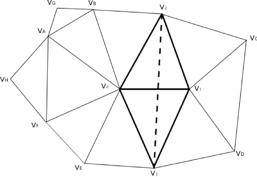
There are two types of hazards when running mesh optimisation algorithms in parallel: structural hazards and data races. The term structural hazards refers to the situation where an adaptive operation results in invalid or non-conforming edges and elements. For example, on the local patch in Figure 4, if two threads flip edges and at the same time, the result will be two new edges and crossing each other. Structural hazards for all adaptive algorithms are avoided by colouring a graph whose nodes are defined by the mesh vertices and edges are defined by the mesh edges. Maximal independent sets are readily selected by calculating the intersection between the set of vertices of each colour and the set of active vertices.
The fact that topological changes are made to the mesh means that after an independent set has been processed the graph colouring has to be recalculated. Therefore, a fast scalable graph colouring algorithm is vital to the overall performance. In this work we use a parallel colouring algorithm described by Gebremedhin et al. [gebremedhin2000scalable]. This algorithm can be described as having three stages: (a) initial pseudo-colouring where vertices are coloured in parallel and invalid colourings are possible; (b) loop over the graph to detect invalid colours arising from the first stage; (c) the detected invalid colours are resolved in serial. Between adaptive sweeps through independent sets it is only necessary to execute stages (b) and (c) to resolve the colour conflicts introduced by changes to the mesh topology.
3.1.3 Deferred operations mechanism
Data race conditions can appear when two or more threads try to update
the same adjacency list. An example can be seen in Figure
6. Having coloured the mesh, two threads
are allowed to process vertices and at the same time
without structural hazards. However, NNList[ ] and
NEList[ ] must be updated. If both threads try to
update them at the same time there will be a data race which could
lead to data corruption. One solution could be a distance-2 colouring
of the mesh (a distance- colouring of is a colouring
in which no two vertices share the same colour if these vertices are
up to edges away from each other or, in other words, if there is a
path of length from one vertex to the other). Although this
solution guarantees a race-free execution, a distance-2 colouring
would increase the chromatic number, thereby reducing the size of the
independent sets and therefore the available parallelism. Therefore,
an alternative solution is sought.
In a shared-memory environment with nthreads OpenMP threads,
every thread has a private collection of nthreads lists, one
list for each OpenMP thread. When NNList[i] or NEList[i]
have to be updated, the thread does not commit the update immediately;
instead, it pushes the update back into the list corresponding to
thread with ID . At the end of the adaptive
algorithm, every thread tid visits the private collections of
all OpenMP threads (including its own), locates the list that was
reserved for tid and commits the operations which are stored
there. This way, it is guaranteed that for any vertex ,
NNList[ ] and NEList[ ] will
be updated by only one thread. Because updates are not committed
immediately but are deferred until the end of the iteration of an
adaptive algorithm, we call this technique the deferred
updates. A typical usage scenario is demonstrated in Algorithm
3.
typedef std::vector<Updates> DeferredOperationsList;
int nthreads = omp_get_max_threads();

// Create nthreads collections of deferred operations lists
std::vector< std::vector<DeferredOperationsList> > defOp;
defOp.resize(nthreads);

#pragma omp parallel
{
  // Every OMP thread executes
  int tid = omp_get_thread_num();
  defOp[tid].resize(nthreads);
  // By now, every OMP thread has allocated one list per thread

  // Execute one iteration of an adaptive algorithm in parallel
  // Defer any updates until the end of the iteration
  #pragma omp for
  for(int i=0; i<nVertices; ++i){
    execute kernel(i);
    // Update will be committed by thread i%nthreads
    // where the modulo avoids racing.
    defOp[tid][i%nthreads].push_back(some_update_operation);
  }

  // Traverse all lists which were allocated for thread tid
  // and commit any updates found
  for(int i=0; i<nthreads; ++i){
    commit_all_updates(defOp[i][tid]);
  }
}
3.1.4 Worklists and atomic operations
There are many cases where it is necessary to create a worklist of items which need to be processed. An example of such a case is the creation of the active sub-mesh in coarsening and swapping, as will be described in Section 3.3. Every thread keeps a local list of vertices it has marked as active and all local worklists have to be accumulated into a global worklist, which essentially is the set of all vertices comprising the active sub-mesh.
One approach is to wait for every thread to exit the parallel loop and then perform a prefix sum [BlellochTR90] (also known as inclusive scan or partial reduction in MPI terminology) on the number of vertices in its private list. After that, every thread knows its index in the global worklist at which it has to copy the private list. This method has the disadvantage that every thread must wait for all other threads to exit the parallel loop, synchronise with them to perform the prefix sum and finally copy its private data into the global worklist. Profiling data indicates that this way of manipulating worklists is a significant limiting factor towards achieving good scalability.
Experimental evaluation showed that, at least on the Intel Xeon, a better method is based on atomic operations on a global integer variable which stores the size of the worklist needed so far. Every thread which exits the parallel loop increments this integer atomically while caching the old value. This way, the thread knows immediately at which index it must copy its private data and increments the integer by the size of this data, so that the next thread which will access this integer knows in turn its index at which its private data must be copied. Caching the old value before the atomic increment is known in OpenMP terminology as atomic capture. Support for atomic capture operations was introduced in OpenMP 3.1. This functionality has also been supported by GNU extensions (intrinsics) since GCC 4.1.2, known under the name fetch-and-add. An example of using this technique is shown in Algorithm 4.
Note the nowait clause at the end of the #pragma omp for
directive. A thread which exits the loop does not have to wait for the
other threads to exit. It can proceed directly to the atomic
operation. It has been observed that dynamic scheduling for OpenMP
for-loops is what works best for most of the adaptive loops in mesh
optimisation because of the irregular load balance across the
mesh. Depending on the nature of the loop and the chunk size, threads
will exit the loop at significantly different times. Instead of having
some threads waiting for others to finish the parallel loop, with this
approach they do not waste time and proceed to the atomic
increment. The profiling data suggests that the
overhead or spinlock associated with atomic-capture operations is insignificant.
int worklistSize = 0; // Points to end of the global worklist
std::vector<Item> globalWorklist;

// Pre-allocate enough space
globalWorklist.resize(some_appropriate_size);

#pragma omp parallel
{
  std::vector<Item> private_list;

  // Private list - no need to synchronise at end of loop.
  #pragma omp for nowait
  for(all items which need to be processed){
    do_some_work();
    private_list.push_back(item);
  }

  // Private variable - the index in the global worklist
  // at which the thread will copy the data in private_list.
  int idx;

  #pragma omp atomic capture
  {
    idx = worklistSize;
    worklistSize += private_list.size();
  }

  memcpy(&globalWorklist[idx], &private_list[0],
             private_list.size() * sizeof(Item));

}
3.1.5 Reflection on alternatives
Our initial approach to dealing with structural hazards, data races and propagation of adaptivity was based on a thread-partitioning scheme in which the mesh was split into as many sub-meshes as there were threads available. Each thread was then free to process items inside its own partition without worrying about hazards and races. Items on the halo of each thread-partition were locked (analogous to the MPI parallel strategy); those items would be processed later by a single thread. However, this approach did not result in good scalability for a number of reasons. Partitioning the mesh was a significant serial overhead, which was incurred repeatedly as the adaptive algorithms changed mesh topology and invalidated the existing partitioning. In addition, the single-threaded phase of processing halo items was another hotspot of this thread-partition approach. In line with Amdahl’s law, these effects only become more pronounced as the number of threads is increased. For these reasons this thread-level domain decomposition approach was not pursued further.
3.2 Refinement
Every edge can be processed and refined without being affected by what
happens to adjacent edges. Being free from structural hazards, the only
issue we are concerned with is thread safety when updating mesh data
structures. Refining an edge involves the addition of a new vertex to the
mesh. This means that new coordinates and metric tensor values have to be
appended to coords and metric and adjacency information in
NNList has to be updated. The subsequent element split leads to the
removal of parent elements from ENList and the addition of new ones,
which, in turn, means that NEList has to be updated as well.
Appending new coordinates to coords, metric tensors to metric
and elements to ENList is done using the thread worklist strategy
described in Section 3.1.4, while updates to
NNList and NEList can be handled efficiently using the
deferred operations mechanism.
The two stages, namely edge refinement and element refinement, of our
threaded implementation are described in Algorithm
5 and Algorithm
6, respectively. The procedure
begins with the traversal of all mesh edges. Edges are accessed using
NNList, i.e. for each mesh vertex the algorithm visits ’s
neighbours. This means that edge refinement is a directed operation, as
edge is considered to be different from edge
. Processing the same physical edge twice is
avoided by imposing the restriction that we only consider edges for
which ’s ID is less than ’s ID. If an edge is found to be
longer than desired, then it is split in the middle (in metric space)
and a new vertex is created. is associated with a pair of
coordinates and a metric tensor. It also needs an ID. At this stage,
’s ID cannot be determined. Once an OpenMP thread exits the edge
refinement phase, it can proceed (without synchronisation with the other
threads) to fix vertex IDs and append the new data it created to the
mesh. The thread captures the number of mesh vertices
and increments it atomically by the number of new vertices it
created. After capturing the index, the thread can assign IDs to the
vertices it created and also copy the new coordinates and metric
tensors into coords and metric, respectively.
Before proceeding to element refinement, all split edges are
accumulated into a global worklist. For each split edge
, the original vertices and have to be
connected to the newly created vertex . Updating NNList
for these vertices cannot be deferred. Most edges are shared between
two elements, so if the update was deferred until the corresponding
element were processed, we would run the risk of committing these
updates twice, once for each element sharing the edge. Updates can be
committed immediately, as there are no race conditions when accessing
NNList at this point. Besides, for each split edge we find the
(usually two) elements sharing it. For each element, we record that
this edge has been split. Doing so makes element refinement much
easier, because as soon as we visit an element we will know
immediately how many and which of its edges have been split. An array
of length NElements stores this type of information.
During mesh refinement, elements are visited in parallel and refined
independently. It should be noted that all updates to NNList
and NEList are deferred operations. After finishing the loop,
each thread uses the worklist method to append the new elements it
created to ENList. Once again, no thread synchronisation is
needed.
This parallel refinement algorithm has the advantage of not requiring any mesh colouring and having low synchronisation overhead as compared with Freitag’s task graph approach.
coords, into metric
NNList[]; replace with in NNList[]
NNList[]
ENList.
ENList.
3.3 Coarsening
Because any decision on whether to collapse an edge is strongly dependent upon what other edges are collapsing in the immediate neighbourhood of elements, an operation task graph for coarsening has to be constructed. Edge collapse is based on the removal of vertices, i.e. the elemental operation for edge collapse is the removal of a vertex. Therefore, the operation task graph is the mesh itself.
Figure 6 demonstrates what needs to be taken into account in order to perform parallel coarsening safely. It is clear that adjacent vertices cannot collapse concurrently, so a distance-1 colouring of the mesh is sufficient in order to avoid structural hazards. This colouring also enforces processing of vertices topologically at least every other one which prevents skewed elements forming during significant coarsening[de1999parallel, li20053d].
An additional consideration is that vertices which are two edges away from each other share some common vertex . Removing both vertices at once means that ’s adjacency list will have to be modified concurrently by two different threads, leading to data races. These races can be avoided using the deferred operations mechanism.
NEList[] NEList[]
NNList[] NNList[]
NEList[].erase() deferred operation
NEList[].erase() deferred operation
NEList[].erase()
ENList[3*] erase element by resetting its first vertex
ENList[3*+{0,1,2}]
NEList[].add() deferred operation
NNList[] deferred operation
NNList[] deferred operation
NNList[]
NNList[] deferred operation
NNList[].clear()
NEList[].clear()
Algorithm 7 illustrates a thread parallel version of mesh edge collapse. Coarsening is divided into two phases: the first sweep through the mesh identifies what edges are to be removed, see Algorithm 8; and the second phase actually applies the coarsening operation, see Algorithm 9. Function coarsen_identify() takes as argument the ID of a vertex , decides whether any of the adjacent edges can collapse and returns the ID of the target vertex onto which should collapse (or a negative value if no adjacent edge can be removed). coarsen_kernel() performs the actual collapse, i.e. removes from the mesh, updates vertex adjacency information and removes the two deleted elements from the element list.
Parallel coarsening begins with the initialisation of array which is defined as:
At the beginning, the whole array is initialised to -2, so that all mesh vertices will be considered for collapse.
In each iteration of the outer coarsening loop, is called for all vertices which have been marked for (re-)evaluation. Every vertex for which is said to be dynamic or active. At this point, a reduction in the total number of active vertices is necessary to determine whether there is anything left for coarsening or the algorithm should exit the loop.
Next up, we find the maximal independent set of active vertices . Working with independent sets not only ensures safe parallel execution, but also enforces the every other vertex rule. For every active vertex which is about to collapse, the local neighbourhood of all vertices formerly adjacent to changed and target vertices may not be suitable choices any more. Therefore, when is erased, all its neighbours are marked for re-evaluation. This is how propagation of coarsening is implemented.
Algorithm 9 describes how the actual coarsening takes place in terms of modifications to mesh data structures. Updates which can lead to race conditions have been pointed out. These updates are deferred until the end of processing of the independent set. Before moving to the next iteration, all deferred operations are committed and colouring is repaired because edge collapse may have introduced inconsistencies.
3.4 Swapping
The data dependencies in edge swapping are virtually identical to those of edge coarsening. Therefore, it is possible to reuse the same thread parallel algorithm as for coarsening in the previous section with slight modifications
In order to avoid maintaining edge-related data structures (e.g. edge-node
list, edge-edge adjacency lists etc.), an edge can be expressed in terms
of a pair of vertices. Just like in refinement, we define an edge
as a pair of vertices , with . We say that
is outbound from and inbound to . Consequently, the edge
can be marked for swapping by adding to .
Obviously, a vertex can have more than one outbound edge, so
unlike in coarsening, in swapping needs
to be a vector of sets (std::vector< std::set<int> >).
The algorithm begins by marking all edges. It then enters a loop which is terminated when no marked edges remain. The maximal independent set of active vertices is calculated. A vertex is considered active if at least one of its outbound edges is marked. Following that, threads process all active vertices of in parallel. The thread processing vertex visits all edges in one after the other and examines whether they can be swapped, i.e. whether the operation will improve the quality of the two elements sharing that edge. It is easy to see that swapping two edges in parallel which are outbound from two independent vertices involves no structural hazards.
Propagation of swapping is similar to that of coarsening. Consider the local patch in Figure 3 and assume that a thread is processing vertex . If edge is flipped, the two elements sharing that edge change in shape and quality, so all four edges surrounding those elements (forming the rhombus in bold) have to be marked for processing. This is how propagation is implemented in swapping.
One last difference between swapping and coarsening is that
needs to be traversed more than once before
proceeding to the next one. In the same example as above, assume that
all edges adjacent to are outbound and marked. If edge
is flipped, adjacency information for ,
and has to be updated. These updates have to be deferred
because another thread might try to update the same lists at the same
time (e.g. the thread processing edge ). However,
not committing the changes immediately means that the thread
processing has a stale view of the local patch. More precisely,
NEList[] and NEList[] are
invalid and cannot be used to find what elements edges
and are part of. Therefore,
these two edges cannot be processed until the deferred operations
have been committed. On the other hand, the rest of ’s outbound
edges are free to be processed. Once all threads have processed
whichever edges they can for all vertices of the independent set,
deferred operations are committed and threads traverse the
independent set again (up to two more times in 2D) to process what
had been skipped before.
3.5 Smoothing
Algorithm 10 illustrates the colouring based algorithm for mesh smoothing. In this algorithm the graph consists of sets of vertices and edges that are defined by the vertices and edges of the computational mesh. By computing a vertex colouring of we can define independent sets of vertices, , where is a computed colour. Thus, all vertices in , for any , can be updated concurrently without any race conditions on dependent data. This is clear from the definition of the smoothing kernel in Section 2.4.4. Hence, within a node, thread-safety is ensured by assigning a different independent set to each thread.
4 Results
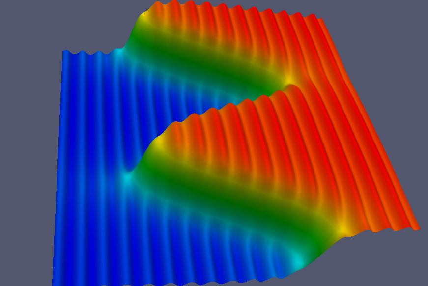
In order to evaluate the parallel performance, an isotropic mesh was generated on the unit square with using approximately vertices. A synthetic solution is defined to vary in time and space:
| (5) |
where is the period. An example of the field at is shown in Figure 7. This is a good choice as a benchmark as it contains multi-scale features and a shock front. These are the typical solution characteristics where anisotropic adaptive mesh methods excel.
Because mesh adaptation has a very irregular workload we simulate a time varying scenario where varies from to in increments of unity and we use the mean and standard deviations when reporting performance results. To calculate the metric we used the -norm as described by [chen2007optimal]. The number of mesh vertices and elements maintains an average of approximately and respectively. As the field evolves all of the adaptive operations are heavily used, thereby giving an overall profile of the execution time.
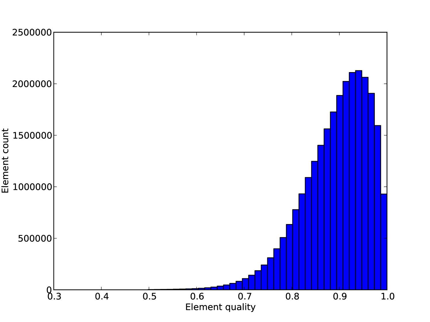
In order to demonstrate the correctness of the adaptive algorithm we plot a histogram (Figure 8) showing the quality of all element aggregated over all time steps. We can see that the vast majority of the elements are of very quality. The lowest quality element had a quality of , and in total only elements out of million have a quality less than .
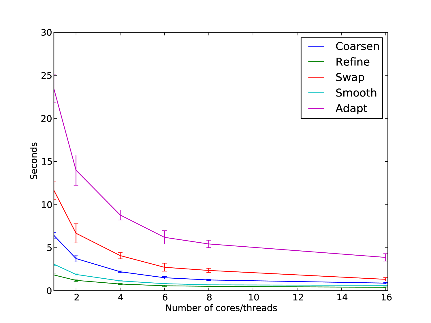
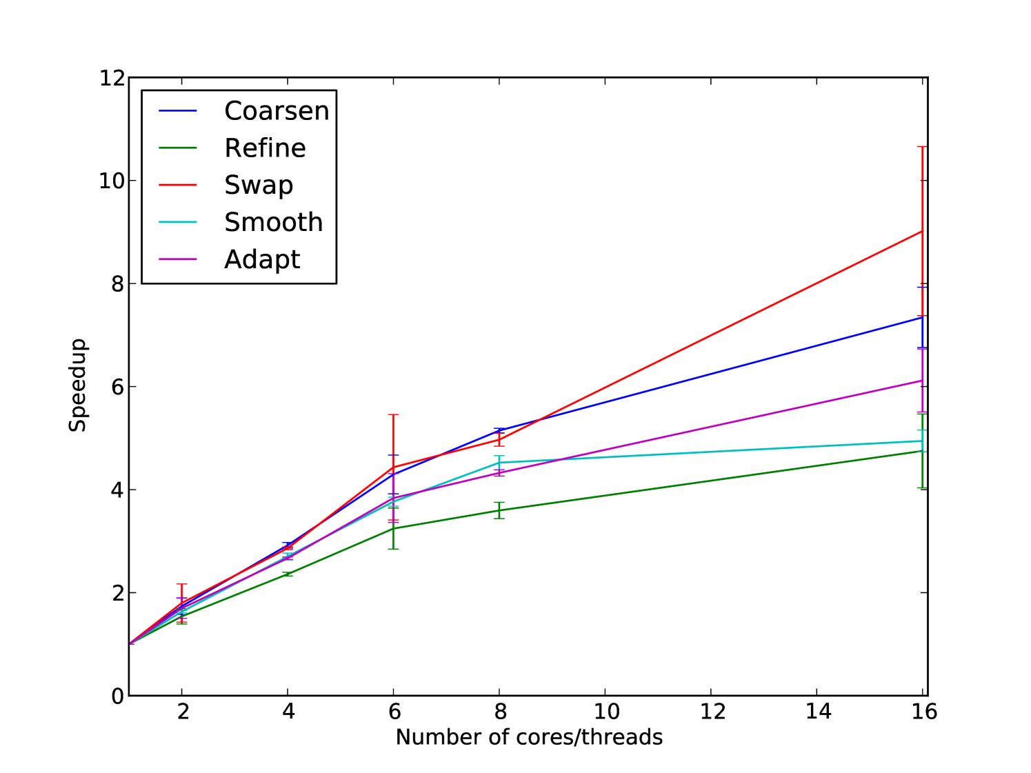
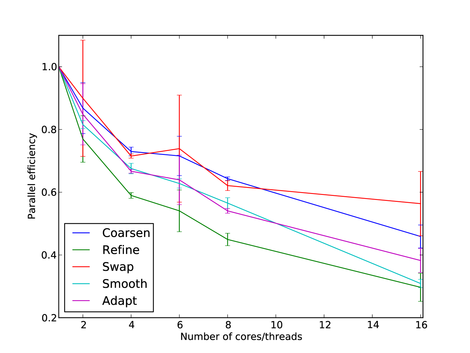
The benchmarks were run on a Intel(R) Xeon(R) E5-2650 CPU. The code was compiled using the Intel compiler suite, version 13.0.0 and with the compiler flags -O3 -xAVX. In all cases thread-core affinity was used.
Figures 9, 10 and 11 show the wall time, speedup and efficiency of each phase of mesh adaptation. Simulations using between 1 and 8 cores are run on a single socket while the 16 core simulation runs across two CPU sockets and thereby incurring NUMA overheads. From the results we can see that all operations achieve good scaling, including for the 16 core NUMA case. The dominant factors limiting scaling are the number of synchronisations and load-imbalances. Even in the case of mesh smoothing, which involves the least data-writes, the relatively expensive optimisation kernel is only executed for patches of elements whose quality falls below a minimum quality tolerance. Indeed, the fact that mesh refinement, coarsening and refinement are comparable is very encouraging as it indicates that despite the invasive nature of the operations on these relatively complex data structures it is possible to get good intra-node scaling.
5 Conclusion
This paper is the first to examine the scalability of anisotropic mesh adaptivity using a thread-parallel programming model and to explore new parallel algorithmic approaches to support this model. Despite the complex data dependencies and inherent load imbalances we have shown it is possible to achieve practical levels of scaling. To achieve this two key ingredients were required. The first was to use colouring to identify maximal independant sets of tasks that would be performed concurrently. In principle this facilitates scaling up to the point that the number of elements of the independant set is equal to the number of available threads. The second important factor contributing to the scalability was the use of worklists and deferred whereby updates to the mesh are added to worklists and applied in parallel at a later phase of an adaptive sweep. This avoids the majority of serial overheads otherwise incurred with updating mesh data structures.
While the algorithms presented are for 2D anisotropic mesh adaptivity, we believe many of the algorithmic details carry over to the 3D case as the challenges associated with exposing a sufficient degree of parallelism are very similar.
6 Acknowledgments
The authors would like to thank Fujitsu Laboratories of Europe Ltd. and EPSRC grant no. EP/I00677X/1 for supporting this work.