A time-modulated Hawkes process to model the spread of COVID-19 and the impact of countermeasures111The simulation code and data used in this work are available under GPL v3 on GitHub: https://github.com/michelegaretto/covid.git
Abstract
Motivated by the recent outbreak of coronavirus (COVID-19), we propose a stochastic model of epidemic temporal growth and mitigation based on a time-modulated Hawkes process. The model is sufficiently rich to incorporate specific characteristics of the novel coronavirus, to capture the impact of undetected, asymptomatic and super-diffusive individuals, and especially to take into account time-varying counter-measures and detection efforts. Yet, it is simple enough to allow scalable and efficient computation of the temporal evolution of the epidemic, and exploration of what-if scenarios. Compared to traditional compartmental models, our approach allows a more faithful description of virus specific features, such as distributions for the time spent in stages, which is crucial when the time-scale of control (e.g., mobility restrictions) is comparable to the lifetime of a single infection. We apply the model to the first and second wave of COVID-19 in Italy, shedding light onto several effects related to mobility restrictions introduced by the government, and to the effectiveness of contact tracing and mass testing performed by the national health service.
keywords:
COVID-19 , Compartmental models, Branching process , Hawkes process1 Introduction and related work
Models of epidemic propagation are especially useful when they provide key insights while retaining simplicity and generality. For example, in mathematical epidemiology the SIR model reveals in very simple terms the fundamental role of the basic reproduction number () which governs the macroscopic, long-term evolution of the outbreak in a homogeneous population. The vast majority of models developed for the novel SARS-CoV-2 are extensions to the classic SIR, along the standard approach of introducing additional compartments to describe different phases of the infection, the presence of asymptomatic, symptomatic or pauci-symptomatic individuals, the set of quarantined, hospitalized people, and so on. Such models lead to a system of coupled ODE’s with fixed or time-varying coefficients to be estimated from traces. A very incomplete list of modeling efforts pursued in this direction, early applied to COVID-19, includes the SEIR models in [1, 2, 3, 4, 5], the SIRD models in [6, 7], the SEPIA model in [8], the SIDHARTE model in [9].
In this paper we develop a slightly more sophisticated model that allows a more accurate representation of native characteristics of a specific virus, such as actual distributions of the duration of incubation, pre-symptomatic and symptomatic phases, for various categories of infected. This level of detail is important when the intensity of applied countermeasures varies significantly over time-scales comparable to that of an individual infection, and we believe it is essential to address fundamental questions such as: i) when and to what extent can we expect to see the effect of specific mobility restrictions introduced by a national government at a given point in time? ii) what is the impact of hard vs partial lockdowns enforced for given numbers of days? when can restrictions be safely released to restart economic and social activities while still keeping the epidemic under control?
Specifically, we propose and analyse a novel, modulated version of the marked Hawkes process, a self-exciting stochastic point process with roots in geophysics and finance [10]. In a nutshell, in the standard marked Hawkes process each event with mark , occurring at time , generates new events with stochastic intensity , where is a generic kernel. The process unfolds through successive generations of events, starting from so-called immigrants (generation zero). In our model events represent individual infections, and a modulating function , which scales the overall intensity of the process at real time , allows us to take into account the impact of time-varying mobility restrictions and social distance limitations. In addition, we model the transition of infected, undetected individuals to a quarantined state at inhomogeneous rate , to describe the time-varying effectiveness of contact tracing and mass testing.
We mention that branching processes of various kind, including Hawkes processes, have been proposed in various biological contexts [11, 12, 13, 14]. In [15], a probabilistic extension of (deterministic) discrete-time SEIR models, based on multi-type branching processes, has been recently applied to COVID-19 to capture the impact of detailed distributions of the time spent in different phases, together with mobility restrictions and contact tracing. In parallel to us, authors of [16] have proposed a Hawkes process with spatio-temporal “covariates” for modeling COVID-19 in the US, together with an EM algorithm for parameter inference. The work in [16] is somehow orthogonal to us, since they focus on spatial and demographic features, aiming at predicting the trend of confirmed cases and deaths in each county. In contrast, we introduce marks and stages to natively model the course of an infection for different categories of individuals, with the fundamental distinction between real and detected cases. Moreover, we take into account the impact of time-varying detection efforts and contact tracing. At last, we obtain analytical expressions for the first two moments of the number of individuals who have been infected within a given time.
We demonstrate the applicability of our model to the novel COVID-19 pandemic by considering real traces related to the first and second wave of coronavirus in Italy. Our fitting exercise, though largely preliminary and based on incomplete information, suggests that our approach has good potential and can be effectively used both for planning counter-measures and to provide an a-posteriori explanation of observed epidemiological curves.
The paper is organized as follows. In Section 2 we provide the mathematical formulation of the proposed modulated Hawkes process to describe the temporal evolution of the epidemic. In Section 3 we motivate our approach by comparing it to the standard SIR model. Some mathematical results related to the moment generating function of our process are presented in Section 4. In Section 5 we describe our COVID-19 model based on the proposed approach. We separately fit our model to the first and second wave of COVID-19 in Italy in Sections 6 and 7, respectively, offering hopefully interesting insights about what happened in this country (and similarly in other European countries) during the recent pandemic. We conclude in Section 8.
2 Mathematical formulation of modulated Hawkes process
We first briefly recall the classic Hawkes process restricted to the temporal dimension (the spatio-temporal formulation is similar, but we focus in this work on the purely temporal version). Events of the process (or points) occur at times , which are -valued random variables. A subset of these points, called immigrants, are produced by an inhomogeneous Poisson process of given intensity . Each immigrant, independently of others, is the originator of a progeny (or cluster) of other points, dispersed in the future through a self-similar branching structure: a first generation of points is produced with intensity , where is the occurrence time of immigrant , and is a kernel function. Each point of the first generation, in turn, generates new offsprings in a similar fashion, creating the second generation of points, and so on.
The above process can be easily extended to account for different types of points with type-specific kernel functions. Types are denoted by marks , which are assumed to be i.i.d. random variables with values on an arbitrary measurable space , with a probability distribution . Let be the counting process associated to the marked points . The (conditional) stochastic intensity of the overall process is then given by:
where is a type-dependent kernel function. In the following we assume to be summable,. i.e.
| (1) |
Note that is the average number of offsprings generated by each point, which is usually referred to as basic reproduction number in epidemiology. The process is called subcritical if , supercritical if .
Our main modification to the above classic marked Hawkes process is to modulate the instantaneous generation rate of offsprings by a positive, bounded function , representing the impact of mobility restriction countermeasures. By so doing, we obtain the modified stochastic intensity of the process:
| (2) |
Note that, when is constant, we re-obtain a classic Hawkes process with modified kernel . In general, the obtained process is no longer self-similar. In particular, the average number of offsprings generated by a point becomes a function of time:
| (3) |
which provides the infamous real-time reproduction number usually referred to on the media as ‘Rt index’.
We emphasize that the process can initially start in the supercritical regime, and then it can become subcritical for effect of a decreasing function , a case of special interest in our application to waves of COVID-19. We mention that the great bulk of literature related to the Hawkes process and its applications to geophysics and finance focuses on the subcritical regime, whereas our formulation applies also to the supercritical regime, which is more germane to epidemics.
The conditional intensity (2) can be easily de-conditioned with respect to , obtaining the ‘average’ stochastic intensity :
| (4) |
where we recall that .
We observe that (2) is a linear Volterra equation of the second kind, which can be efficiently solved numerically.222For example, the standard trapezoidal rule allows obtaining a discretized version of by a matrix inversion. In the special case of constant modulating function, (2) reduces to a convolution equation which can be analyzed and solved by means of Laplace transform techniques (see A).
At last we introduce the total number of points up to time , (regardless of their associated marks), and its average:
| (5) |
3 Comparison with SIR model
When the kernel function has an exponential shape, i.e., , it is possible to establish a simple connection between the Hawkes process and the classic SIR model [17]. Specifically, consider a stochastic SIR model with an infinite population of susceptible individuals, where each infected generates new infections at rate , and recovers at rate (i.e., after an exponentially distributed amount of time of mean ). Then the average intensity of the process generated by this stochastic SIR, averaging out the times at which nodes recover, has exactly the (conditional) intensity of a Hawkes process starting with the same number of initially infected nodes, no further immigrants, and [17]. This can be intuitively understood by considering that in SIR the average, effective rate with which an infected individual generates new infections after time since it became infected equals times the probability that the node has not yet recovered, which is .
We remark that in [17] authors push this equivalence a bit further, by showing that a SIR model with finite population is equivalent to a modulated Hawkes process similar to (2), where . In our model and its application to COVID-19, we do not consider the impact of finite population size, and assume an infinite population of susceptible individuals333This assumption is largely acceptable at the beginning of an epidemic.. Therefore, we do not need the ‘correction factor’ , and instead use the modulating function to model the (process-independent) effect of mobility restrictions. A similar effect due to mobility restrictions can be incorporated into the SIR model, by applying factor to the infection rate .
Given the above connection between a (possibly modulated) Hawkes process and the traditional SIR, one might ask what is the benefit of our approach with respect to SIR-like models. In contrast to SIR, the Hawkes process allows us to choose an arbitrary kernel , not necessarily exponential. With this freedom, can we observe dynamics significantly different from those that can be obtained by a properly chosen exponential shape? We answer this question in the positive with the help of an illustrative scenario.
Consider an epidemic starting at time zero with infected individuals.444Note that in our model the number of immigrants has a Poisson distribution with mean . However to reduce the variance we have preferred to start simulations with the same deterministic number of infected. Further, note that analytical results for the mean trajectory of infected nodes are not affected by this choice. We fix to (days) the average generation time, which is the mean temporal separation between a new infection belonging to generation and its parent in generation . Note that the above constraint implies that .
We also normalize , since we can use to scale the infection rate, in addition to considering time-varying effects due to mobility restriction. Note that in SIR we can only satisfy the above constraints by choosing the exponential kernel , . Instead, in our Hawkes model we have much more freedom.
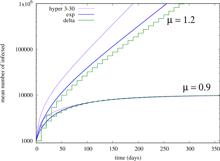
First, we consider a scenario in which is constant, equal to either 1.2 (supercritical case) or 0.9 (subcritical case). In Fig. 1 we show the temporal evolution of the mean number of infected , for three kernel shapes that allows for an explicit solution of (2),(5) using Laplace transform (A). The delta shape corresponds to the kernel function , where is Dirac’s delta function, for which
| (6) |
The exp shape corresponds to the exponential kernel (SIR model), for which
| (7) |
The hyper shape corresponds to the hyper-exponential kernel:
,
where , , ,
which also permits obtaining an explicit, though lengthy expression of that we omit here.
Specifically, the ‘hyper’ curve on Fig. 1 corresponds
to the case , .
We observe that, in the subcritical case (), the mean number of infected saturates to the same value, irrespective of the kernel shape; this can be explained by the fact that the final size of the epidemics is described by the same branching process for all kernel shapes (i.e., a branching process in which the offspring distribution is Poisson with mean 0.9). In the supercritical case (), instead, the mean number of infected grows exponentially as (as grows large), where, interestingly, depends on the particular shape (notice the log axes on Fig. 1). In particular, the hyper-exponential kernel can produce arbitrarily large (A). We conclude that, even when we fix the average generation time , different kernels can produce largely different (in order sense) evolutions of . Note that, by introducing compartments, SIR-like models can match higher-order moments of the generation time, but our results suggest that depends on all moments of it, i.e., on the precise shape of the kernel. Moreover, recall that some shapes are difficult to approximate by a phase-type approximation (e.g., the rectangular shape, or more in general, kernels with finite support).
The strong impact of the specific kernel shape becomes even more evident when we consider a time-varying , as in our modulated Hawkes process. As an example, consider the COVID-inspired scenario in which the modulating function corresponds to the black curve in Fig. 2: during the first 30 days, decreases linearly from 3 to 0.3; it stays constant at 0.3 for the next 60 days; and it goes back linearly to 3 during the next 30 days, after which it stays constant at .
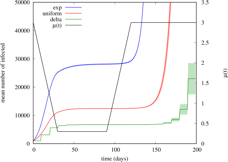
In Fig. 2 we show the mean number of infected estimated by simulation (averaging 100 independent runs), for the three kernel shapes exp, delta, and uniform, where uniform corresponds to the kernel , , while the shapes exp, delta have been already introduced above. Shaded areas around each curve denote level confidence intervals.
We observe huge discrepancies among the trajectories of obtained under the three kernels. In particular, after the first ‘wave’ of 30 days, the exp kernel produces about four times more infections than those produced by the delta kernel. This can be explained by the fact that varies significantly on a time window (30 days) comparable to the average generation time (10 days).
It is also interesting to compare what happens on the second wave starting at day 90, after all 3 curves have settled down to an almost constant value: now discrepancies are even more dramatic: although we observe a very fast resurgence of the epidemic in all cases, this happens with significant delays from one curve to another. This is due to the fact that the number of individuals who are still infectious after the subcritical period (when ) is largely different, especially considering that both the uniform and delta kernels have finite support (20 and 10 days, respectively) much smaller than the duration of the subcritical period, whereas the exp shape has infinite support: this implies that under the uniform and delta kernels the virus survives the subcritical period only through chains of infections belonging to successive generations, whereas under the exp shape in principle the epidemic can restart just thanks to the original immigrants at time 0, who are still weakly infectious when we re-enter the supercritical regime (around day 100). Actually, in our experiment, under the delta kernel the epidemic died out in 68 out of 100 simulation runs, which explains the large confidence intervals obtained in this case at end of the observation window. Under the uniform kernel, the epidemic died only in 3 out of 100 runs, while it always survived under the exp kernel.
We conclude that, even while fixing the mean generation time, the precise shape of the kernel function can play an important role in predicting the process dynamics and the impact of countermeasures, especially when the time-scale of control is comparable to the time-scale of an individual contagion. One might obtain a good fitting with measured data also by using an exponential shape, and a properly chosen modulating function , but this is undesirable, since the required would no longer reflect the actual evolution of mobility and interpersonal contact restrictions. In the case of COVID-19, several researchers have actually attempted to incorporate into analytical models detailed information about people mobility, using for example data provided by cellular network operators or smartphone apps [18, 19].
4 Moment generating function
Our modulated Hawkes process is stochastic in nature, hence it is important to characterize how realizations of the process are concentrated around the mean trajectory derived in Sec. 2. This characterization is instrumental, for example, in designing simulation campaigns with proper number of runs. Moreover, note that it is entirely possible that the epidemic gets extinct at its early stages, or in between two successive waves, as we have seen in the scenario in Fig. 2. Actually, an epidemic could die out even when starting in the supercritical regime (consider the case of a single immigrant at time , who does not generate any offspring with probability ), something that is not captured by deterministic mean-field approaches. Therefore, it is interesting to understand the variability of the process at any time.
Under mild assumptions an expression for the moment generating function of the number of points in can be given, and an iterative procedure can be applied to compute the moment of any order in terms of moments of smaller order, though with increasing combinatorial complexity.
In this section we limit ourselves to reporting the main results on this moments’ characterization, without their mathematical proofs, to keep the paper focused on the application to COVID-19 and its control measures.
Hereon, we shall assume
| (8) |
Also, we fix a horizon , and, for , we denote with the number of points, up to time , in the cluster generated by an immigrant at (including the immigrant). We denote with the modulus of a complex number.
We are interested in , i.e., the total number of points generated up to time , irrespective of their mark.
Theorem 4.1 (Moment generating function of )
From the moment generating function we can obtain an expression for the first and second moment of (the first moment can also be obtained directly from the average stochastic intensity, as we have done in Sec. 2.).
Theorem 4.2 (The first two moments of )
| (13) |
and
| (14) |
with
| (15) |
| (16) |
and
| (17) |
5 COVID-19 Model
Now we describe how we applied the modulated Hawkes process introduced before to model the propagation dynamics of COVID-19. The proposed model could actually be used to represent the dynamics of other similar viruses as well.
First, we take advantage of the fact that we do not need to consider a unique kernel function for all infected. Indeed, the presence of marks allows us to introduce different classes of infectious individuals with specific kernel functions. Specifically, we have considered three classes of infectious: symptomatic, asymptomatic and superspreader, denoted by symbols . We assume that, when a person gets infected, it is assigned a random class with probabilities , respectively, , , , .
As the name suggests, symptomatic people are those who will develop evident symptoms of infection, and we assume that because of that they will be effectively quarantined at home or hospitalized at the onset of symptoms. On the contrary, the asymptomatic mark is given to individuals who will not develop strong enough symptoms to be quarantined. Therefore, they will be able to infect other people for the entire duration of the disease, though at low infection rate (unless they get scrutinized by mass testing, as explained later). At last, superspreaders are individuals who exert a high infection rate but do not get quarantined due to several possible reasons (unless they get scrutinized by mass testing). This class also includes people with mild symptoms, who become highly contagious because of their mobility pattern (e.g., participation to ‘superspreading events’). Though the above classification of infectious individuals is a simplified one, a properly chosen mix of the three considered classes can represent a wide range of different scenarios.
Irrespective of their class, we will assume that all infectious people go through the following sequence of stages: first, there is a random incubation time, denoted by r.v. , with given cdf . During this time we assume the all infected exert a low infection rate . Then, there is a crucial pre-symptomatic period, during which infected in classes already exert a high infection rate , while infected in class still exert low infection rate . For simplicity, we have assumed the presymptomatic phase to have constant duration .
The following evolution of the infection rate of an individual depends on the class: since we assume that symptomatic people get effectively quarantined, they no longer infect other individuals after the onset of symptoms. We model this fact introducing a quarantined class of people (denoted by ), and deterministically moving all infected in class to class after time .
People in classes continue to be infectious during a disease period of random duration , with given cdf . The difference between these two classes is that infectious in class () exert, during the disease period, infection rate (), respectively. At last, we assume that people in classes enter a residual period of random duration , with cdf , during which all of them exert infection rate . We introduced this additional phase because some people who recovered from COVID-19 where found to be still contagious several days (even weeks) after the end of the disease period. Note that durations are assumed to be independent, and that the complete mark associated to an infected is the tuple .
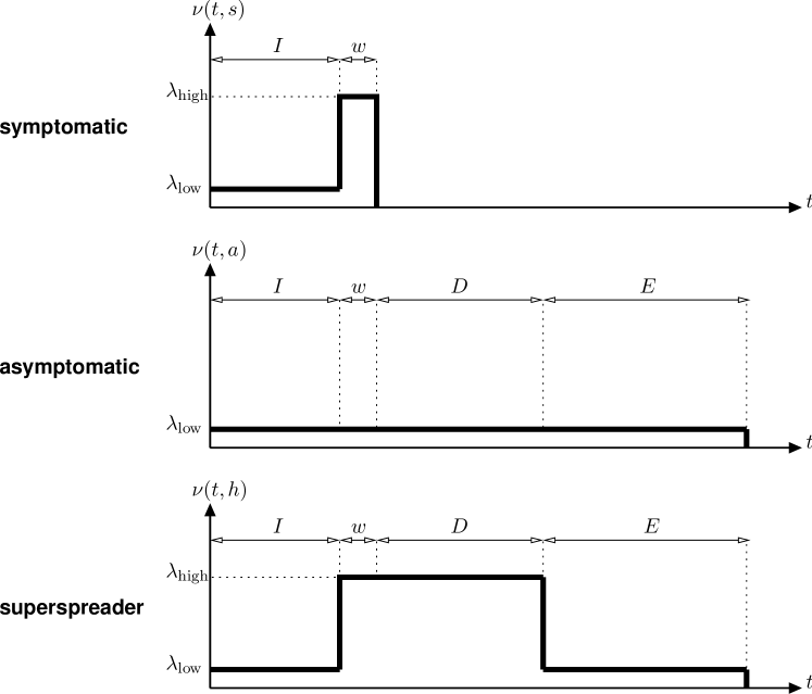
An illustration of the three class-dependent kernels , conditioned on the durations , is reported in Fig. 3.
Remark 5.1
We emphasize that our model of COVID-19 is targeted at predicting the process of new infections, rather than the current number of people hosting the virus in various conditions. In particular, we do not explicitly describe the dynamics of symptomatic but quarantined people and their exit process (i.e., recovery or, in the worst case, death), since such dynamics have no effect on the spreading process (under the assumption of perfect quarantine). However, if desired, one could describe through appropriate probabilities and time distributions how quarantined people split between those isolated at home and those who get hospitalized, the fraction going to intensive care, and those who unfortunately die.
| Parameter | symbol | COVID-19 fitted value |
|---|---|---|
| incubation period | I | tri([2,12], mean 6) |
| pre-symptoms period | w | 2 |
| disease period | D | unif([2,12]) |
| residual period | E | exp(10) |
| low infection rate | 0.05 | |
| high infection rate | 1 | |
| symptomatic probability | 0.06 | |
| asymptomatic probability | 0.91 | |
| super-spreader probability | 0.03 |
The parameters introduced so far, summarized in Table 1, are related to specific characteristics of the virus. We now model properties of the specific environment where the virus spreads, taking into account the impact of countermeasures. First, we need to specify the immigration process . To keep the model as simple as possible, we have assumed that the system starts at a given time with new infections, i.e., immigrants arrive as a single burst concentrated at one specific instant.
The impact of countermeasures is taken into account in the model in two different ways. First, modulating function can be used to model the instantaneous reduction of the infection rate at time due to the current mobility restrictions, and, more in general, changes in the environment which affect the ability of the virus to propagate in the susceptible population (such as seasonal effects). Typically, is a decreasing function in the initial part of the epidemics, in response to new regulations introduced by the government, while it goes up again when mobility restrictions are progressively released.
Second, we assume that any infected not already found to be positive is tested (e.g., by means of massive swab campaigns) at individual, instantaneous rate , which reflects both the amount of resources employed by the health service to discover the infected population, and the effectiveness of tracking. Recall that, when an infected is found positive, we assume it transits to the quarantined state and stops infecting other people.
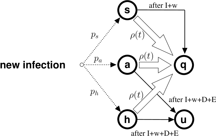
Fig. 4 shows the resulting transitions that can occur for the different classes. Note that class collects all cases known to the health authorities at a given time , and thus coincides with the set of detected cases. Infected in classes are still unknown to the health service (but they are detectable). When they stop to be positive, people in classes transit to a class (undetected), which collects all infected who remain unknown to the health service.
Environment-related parameters are summarized in Table 2.
| Parameter | symbol | fitted value for first wave in Italy |
|---|---|---|
| initial day | -20 | |
| initial number of infected | 370 | |
| modulating function | , | |
| , , (see Fig. 5) | ||
| detection rate | , (see Fig. 5) |
Remark 5.2
We emphasize that the model described so far does not explicitly model spatial effects and sub-populations. As such, it is more suitable to describe a homogeneous scenario, where its environmental parameters (including modulating functions and detection rate ) can be reasonably assumed to apply to all individuals of the population irrespective of their spatial location. The natural candidate of such scenario is a single nation or just a sub-region of it. By so doing, we can assume that common national regulations are applied, as well as common health-care practices. However, our approach based on Hawkes processes could be extended to incorporate spatial effects, by considering spatio-temporal kernel functions , where is a spatial vector originated at the point at which a new infection occurs. Another possibility would be to consider a multivariate temporal Hawkes process, where each component represents a homogeneous region, and the different regional processes can interact with each other.
5.1 Computation of the real-time reproduction number
From our model, it is possible to compute in a native way the average number of infections caused by an individual who gets infected at time , i.e., the real-time reproduction number . To compute , we condition on the duration of the incubation time, on the duration of the disease time, on the duration of the residual time, and on the class assigned to the node getting infected at time (note that they are all independent of each other):
| (18) |
where
is the probability that a node which gets infected at time is still undetected at time .
6 Model fitting for the first wave of COVID-19 in Italy
We fit the model to real data related to the spread of COVID-19 in Italy, publicly available on GitHub [20]. Italy was the country where the epidemics first spread outside of China into Europe, causing about 34600 deaths at the end of June 2020 during the first wave.
Our main goal was to match the evolution of the number of detected cases, represented in the model by individuals in class . The actual count is provided by the Italian government on a daily basis since February 24th 2020. We take this date as our reference day zero. However, it is largely believed that the epidemics started well before the end of February. Indeed, it became soon clear that detected cases were just the top of a much bigger iceberg, as the prevalence of asymptomatic infection was initially largely unknown, which significantly complicated the first modeling efforts to forecast the epidemic evolution. During June-July 2020, a blood-test campaign (aimed at detecting IgG antibodies) was conducted on a representative population of 64660 people to understand the actual diffusion of the first wave of COVID-19 in Italy [21]. As a main result, it has been estimated that 1 482 000 people have been infected. This figure provides a fundamental hint to properly fit our model, and indeed while exploring the parameter space we decided to impose that the total number of predicted cases at the end of June (day 120) is roughly 1 500 000.
For the durations ,,, of the different stages of an infection, we have tried to follow estimates in the medical literature. In particular, the duration of the incubation period is believed to range between 2 and 12 days, with a sort of bell shape around about 5 days [22, 23, 24], which we have approximated, for simplicity, by a (asymmetric) triangular distribution with support and mean 6. Moreover, we have fixed the duration of the pre-symptomatic phase to 2 days. For the duration of the disease period we have taken a uniform distribution on , while the residual time is modeled by an exponential distribution with mean 10 days [25].
The other virus-related parameters have been set as reported in the third column of Table 1. Note that, since we further apply the external modulating function , we could arbitrarily normalize to 1 the value of , while we set .
For what concerns environment-related parameters (see Table 2), a first problem was to choose a proper initial day (recall that day zero is the first day of the trace) at which to start the process with initially infected individuals. While different pairs are essentially equivalent, we decided not to start the process with too few cases and too much in advance with respect to day 0, to limit the variance of a single simulation run. We ended up setting , while was selected as explained later.

Mobility restrictions in Italy were progressively enforced by national laws starting a few days before day 0, first limited to red zones in Lombardy, and soon extended to the entire country through a series of increasingly restrictive regulations, introduced over the next 30 days. Instead of trying the capture the step-wise nature of such restrictions, we assume to take the simpler profile depicted in Figure 5, i.e., a high initial value before time , a low final value after time , and a linear segment connecting point to point . We decided to set and to reflect the time window in which mobility restriction were introduced.
In Fig. 5 we also show our choice for the profile of detection rate , i.e., a linear increase starting from day 0, with coefficient , . This profile is justified by the fact that the first wave caught Italy totally unprepared ( before day zero), while massive swabs were only gradually deployed over time after day zero.
The critical parameters were fitted by a minimum mean square error (MMSE) estimation technique based on the curve of detected cases in the time window days, after all other parameters were manually selected as detailed above.
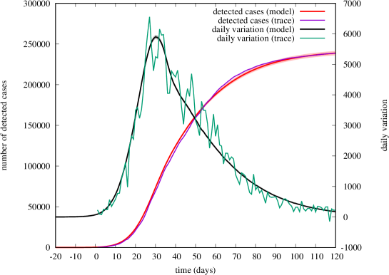
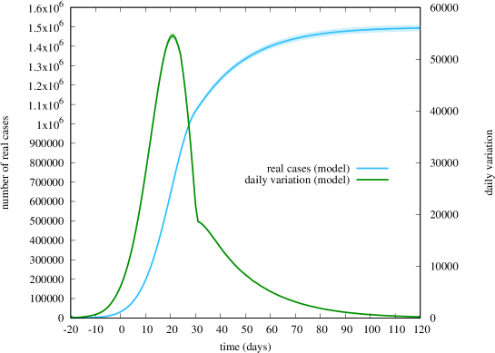
Fig. 6 shows the final outcome of our fitting, comparing the evolution of the number of detected cases according to model and real data. We show both the cumulative number (left axes) and its daily increment (right axes). Analytical predictions for the mean trajectory of detected cases were obtained by averaging 100 simulation runs. The shaded region around analytical curves (barely visible) shows 95%-level confidence intervals computed for each of the 120 days.
We emphasize that a similar good match could be possibly obtained by other sets of parameters. Our purpose here was not to compute the best possible fit in the entire parameter space (which would be nearly impossible), but to show that the model is rich enough to capture the behavior observed on the real trace after a reasonable choice of most of its parameters, driven by their physical meaning.
Fig. 7 shows instead the evolution of the real number of cases (both the cumulative number and its daily variation) according to the model only, in the absence of data. Note however that we have constrained ourselves to obtain a total number of about 1 500 000 cases on day 120, as suggested by the serological test [21].
Interestingly, by looking at the values of and computed by our MMSE, it appears that the national lockdown was able to reduce the spreading ability of the virus within the Italian population by a factor of about 12 (from 3.71 to 0.31). We will see later on in Fig. 12 that our fitting of for the first wave is consistent with mobility trends estimated from the usage of the Apple maps application [19].
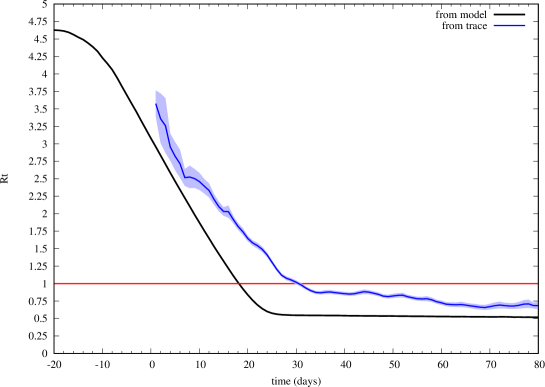
In Fig. 8 we show the real-time reproduction number computed by (18). We also applied the classic method of Wallinga-Teunis [26], implemented as in the R0 package [27], to estimate from the trace of detected cases. To apply their method, we used a generation time obtained from a Gamma distribution with mean 6.6 (shape 1.87, scale 0.28), which has been proposed for the first wave of COVID-19 in Italy [28]. Interestingly, though both estimates of exhibit qualitatively the same behavior, the model-based value of , which considers also undetected cases, tends to be smaller.
6.1 What-if scenarios
Having fitted the model to the available trace, we proceed to exploit the model to examine interesting what-if scenarios. First, we investigate what would have happened (according to the fitted model) if lockdown restrictions were shifted in time by an amount of days . This means that we keep all parameters the same, except that we translate horizontally in time the profile of depicted in Fig. 5. In Figure 9 we show the total number of cases that would have occurred for values of .
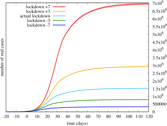
We observe that a shift of just 3 days corresponds to a factor of roughly 2 in the number of cases. This translates, dramatically, into an equivalent impact on the number of deaths, if we assume that the mortality rate would have stayed the same555This is somehow optimistic, since mortality also depends on the saturation level of intensive therapy facilities. (i.e., ). In other words, a postponement (anticipation) of lockdown restrictions by just 3 days wold have caused twice (half) the number of deaths, which is a rather impressive result.
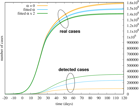
In Figure 10 we investigate instead the impact of detection rate , by changing its slope (recall Fig. 5). We report both the number of real cases and the number of detected cases predicted by the model, when all other fitted parameters are kept the same. We consider what would have occurred with (which means that infectious people are never tested), and by doubling the intensity of the detection rate (a tracking system twice more efficient). As expected, with only symptomatic cases () are eventually detected. This time the effect on the final number of cases (or deaths) is not as dramatic as in the previous what-if scenario. This suggests that the impact of mass testing in Italy during the first wave was marginal, and doubling the efforts would not have produced significant changes in the final outcome.
7 Model fitting for the second wave of COVID-19 in Italy
The second wave of COVID-19 hit Italy in late summer 2020, as in many other European countries, mainly as en effect of relaxed mobility in July/August and possibly other seasonal effects. It is interesting to compare the second wave with the first wave, by looking at the daily increments of detected cases and deaths, see Fig. 11.
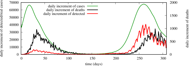
We observe that the number of daily deaths is similar between the two waves. The daily increment of detected cases, instead, is very different (around 5000 at the peak of the first wave, around 35000 at the peak of the second wave, a 7-fold increase). This can be explained by the much larger capacity of the health service to perform swabs and track down the infected, built on the experience gained from the first wave. It also suggests that, differently from the first wave, the impact of (the individual rate at which an infectious is detected) is expected to be much more important during the second wave than in the first wave, requiring a careful treatment of it in the model.
We have indeed tried to fit our model to the second wave in Italy, keeping all parameters related to the virus (previously fitted for the first wave) unchanged (Table 1), and adapting only environment-specific parameters (Table 2). A major difficulty that we had to face was the unknown (at the time of writing) actual diffusion of the virus in the population during the second wave. Recall that, for the first wave, we exploited a blood-test campaign to get a reference for the total number of real cases at the end of the first wave. For the second wave we employed instead a different approach based on a projection back in the past of the increment of deaths. A similar idea has been adopted in [29] to estimate the time-varying reproduction number in different European country at the onset of the first wave.
Specifically, we got from [30] the indication of the median (11 days) and IQR (6-18 days) of the amount of time from symptoms onset to death during Oct-Dec 2020, that we fitted by a Gamma distribution (shape 1.65, scale 8.45). By convolving such Gamma distribution with the distribution of incubation time, and the pre-symptoms period, we obtained a distribution of the total time from infection to death, that we used to estimate the time in the past at which each dead person was initially infected. By amplifying the number of infections leading to death by the inverse of the mortality rate we eventually obtained an estimate of the daily increment of real cases, as reported in Fig. 11 (green curve, left -axes).
We chose August 1st (day 160 on Fig. 11) as starting date of the new infection process producing the second wave in Italy. This time, instead of manually searching for suitable profiles of and generating the expected curves of real and detected cases, we adopted a novel “reverse-engineering” approach: we took the daily increments of real and detected cases as input to the model, and computed the functions and that would exactly produce in the model the given numbers of real and detected cases, on each day666Discretized values of functions and are uniquely determined in the model, once we constrain ourselves to produce a given number of real and detected cases at each time instant..
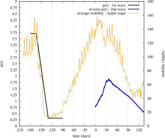
In Fig. 12 we show the obtained ‘reversed’ (blue curve), starting from day 0 (August 1st) of the time reference adopted for the second wave. We also report the average mobility measured in Italy by the Apple maps application [19], where we have given equal weight (1/3) to driving, transit and walking mobility. We observe that the ‘reversed’ qualitatively follows the same behavior of mobility measured on the maps application, with a gradual increase during the month of August followed by a gradual decrease as people (and the government) started to react to the incipient second wave.
For completeness, we have also reported on Fig. 12 the fitted for the first wave (black curve). We observe that, during the first wave, the quick introduction of hard lockdown caused an abrupt decay of both measured mobility and fitted , characterized by a bigger reduction in a shorter time. The second wave, instead, was characterized by a smoother transition, due to the different choice of applying just partial lockdowns and progressive restrictions more diluted over time777The fact that, during the second wave, mobility values similar to those of the first wave do not translate into equally similar values of can be attributed to increased awareness of people during the second wave..
In Fig. 13 we show instead the ‘reversed’ function , focusing on the second wave. We also report on the same plot the daily increments of real and detected cases, which allow us to better understand the obtained profile of , highlighting an interesting phenomenon occurred around day 30. Indeed, we observe that, during the first month, the epidemic was closely tracked by the national health system, but at some point, around day 30, the curve of detected cases stops increasing, and stays roughly constant during the entire second month, lagging more and more behind the otherwise exploding curve of real cases (time window 30-60). As consequence, function , which describes the effectiveness of individual tracking, falls down to a minimum reached at around day 60. This behavior can be interpreted as an effect of the saturation of the capacity to perform swabs, resulting in a progressive collapse of the tracking system, as actually experienced by many people during those days.
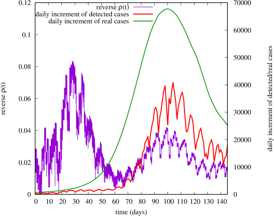
Our analysis shows that, in contrast to what might be believed by just looking at the curve of detected cases, September (days 30-60) was, perhaps, the most critical period for the outbreak of the second wave of COVID-19 in Italy. During this period, the detection capacity of the national health system was saturated, and could not keep the pace with the rapid growth of real cases, giving instead the illusion of maintaining the epidemic under control. Our reverse-engineering approach can thus shed some light on what actually happened at the onset of the second wave, and quantitatively assess the collapse of the tracking system.
8 Conclusions
We have proposed a time-modulated version of the Hawkes process to describe the temporal evolution of an epidemic within an infinite population of susceptible individuals. Our approach allows us to take into account precise distributions for the time spent in different stages of the infection, which is of paramount importance when the intensity of countermeasures (mobility restrictions, testing and tracing) varies significantly on time-scales comparable to that of an individual infection. We have applied the model to the spread of COVID-19 in Italy, either by a direct fit of its parameter (first wave), or by a novel reverse fit (second wave) which allows us, in retrospect, to understand from data the time-varying effectiveness of applied countermeasures. Future work will extend the model to overcome some of its current limitations, like the impact of spatial effects and other sources of heterogeneity in the population, such as age groups. We think the proposed approach is promising and could be usefully applied to explain the epidemic progress and forecast/assess the impact of control/mitigation measures.
Appendix A Explicit solution of for constant
When is constant, denoting with the convolution product, we can rewrite equation (2) as
which can be easily solved in the transformed domain. For a non-negative function , we denote by
the Laplace transform of . Then we have:
with equal to the zero of with largest real part.
In addition, formally, as long as and is bounded, we can write
where is the -th fold convolution of .
An analytical expression of can be obtained when and are both rational. Table 3 reports the dominant888 We recall that a non negative function is said to be , iff there exist two constants such that , for sufficiently large . term of (and also of ) for the case in which , and takes different shapes satisfying:
| shape | ||
|---|---|---|
| delta | ||
| erl- | ||
| exp | ||
| hyper1 | ||
| hyper2 |
Besides the simple deterministic (delta) and exponential (exp) shapes, we consider the Erlang-2 (erl-) and two variants of hyper-exponential, whose general form is . To reduce the degrees of freedom of the general hyper-exponential, we have assumed a particular relationship between and , which allows us to introduce a single parameter . Specifically, we have set either (denoted by hyper1) or (denoted by hyper2). Note that in both cases the variance of the corresponding hyper-exponential distribution increases with , becoming arbitrarily large as .
For all kernel shapes, and , the growth rate of is exponential, i.e., , and the same holds for . The rate of the exponential growth, however, depends on the specific shape.
In particular, for the two considered cases of hyper-exponential shape, is an increasing function of : while in the hyper1 case saturates to , as , in the hyper2 case is even unbounded, as .
We also notice that the rate of the exponential kernel is larger than the rate of the Erlang-2 kernel, which is in turn larger than the rate of the deterministic kernel.
These results confirm that, even under a constant modulating function , the epidemic growth rate depends on the specific shape of the kernel function .
References
-
[1]
Y. Fang, Y. Nie, M. Penny,
Transmission dynamics of the
COVID-19 outbreak and effectiveness of government interventions: A
data-driven analysis, Journal of medical virology 92 (6) (2020) 645–659,
32141624[pmid].
URL https://pubmed.ncbi.nlm.nih.gov/32141624 -
[2]
A. J. Kucharski, T. W. Russell, C. Diamond, Y. Liu, J. Edmunds, S. Funk, R. M.
Eggo, F. Sun, M. Jit, J. D. Munday, N. Davies, A. Gimma, K. van Zandvoort,
H. Gibbs, J. Hellewell, C. I. Jarvis, S. Clifford, B. J. Quilty, N. I. Bosse,
S. Abbott, P. Klepac, S. Flasche,
Early
dynamics of transmission and control of COVID-19: a mathematical modelling
study, The Lancet Infectious Diseases 20 (5) (2020) 553 – 558.
URL http://www.sciencedirect.com/science/article/pii/S1473309920301444 -
[3]
S. Pei, J. Shaman,
Initial
Simulation of SARS-CoV2 Spread and Intervention Effects in the Continental
US, medRxiv (2020).
URL https://www.medrxiv.org/content/early/2020/03/27/2020.03.21.20040303.full.pdf -
[4]
D. Zou, L. Wang, P. Xu, J. Chen, W. Zhang, Q. Gu,
Epidemic
Model Guided Machine Learning for COVID-19 Forecasts in the United States,
medRxiv (2020).
URL https://www.medrxiv.org/content/early/2020/05/25/2020.05.24.20111989.full.pdf -
[5]
A. C. Miller, N. J. Foti, J. A. Lewnard, N. P. Jewell, C. Guestrin, E. B. Fox,
Mobility
trends provide a leading indicator of changes in SARS-CoV-2 transmission,
medRxiv (2020).
URL https://www.medrxiv.org/content/early/2020/05/11/2020.05.07.20094441.full.pdf -
[6]
C. Anastassopoulou, L. Russo, A. Tsakris, C. Siettos,
Data-based analysis,
modelling and forecasting of the COVID-19 outbreak, PLOS ONE 15 (3) (2020)
1–21.
URL https://doi.org/10.1371/journal.pone.0230405 -
[7]
G. C. Calafiore, C. Novara, C. Possieri,
A
time-varying SIRD model for the COVID-19 contagion in Italy, Annual Reviews
in Control 50 (2020) 361 – 372.
URL http://www.sciencedirect.com/science/article/pii/S1367578820300717 -
[8]
M. Gatto, E. Bertuzzo, L. Mari, S. Miccoli, L. Carraro, R. Casagrandi,
A. Rinaldo, Spread
and dynamics of the COVID-19 epidemic in Italy: Effects of emergency
containment measures, Proceedings of the National Academy of Sciences
117 (19) (2020) 10484–10491.
URL https://www.pnas.org/content/117/19/10484.full.pdf -
[9]
G. Giordano, F. Blanchini, R. Bruno, P. Colaneri, A. Di Filippo, A. Di Matteo,
M. Colaneri, Modelling the
COVID-19 epidemic and implementation of population-wide interventions in
Italy, Nature Medicine 26 (6) (2020) 855–860.
URL https://doi.org/10.1038/s41591-020-0883-7 -
[10]
A. G. Hawkes, Spectra of Some
Self-Exciting and Mutually Exciting Point Processes, Biometrika 58 (1)
(1971) 83–90.
URL http://www.jstor.org/stable/2334319 - [11] A. D. Kimmel M., The Bellman-Harris Process, Branching Processes in Biology, Interdisciplinary Applied Mathematics, Springer, New York, NY 19 (2002) 87–102. doi:https://doi.org/10.1007/0-387-21639-1_5.
- [12] H. Mei, J. Eisner, The Neural Hawkes Process: A Neurally Self-Modulating Multivariate Point Process, in: Proceedings of the 31st International Conference on Neural Information Processing Systems, NIPS’17, Curran Associates Inc., Red Hook, NY, USA, 2017, p. 6757–6767.
-
[13]
M. Kim, D. Paini, R. Jurdak,
Modeling stochastic
processes in disease spread across a heterogeneous social system,
Proceedings of the National Academy of Sciences 116 (2) (2019) 401–406.
URL https://www.pnas.org/content/116/2/401.full.pdf -
[14]
H. Xu, H. Zha,
A
Dirichlet Mixture Model of Hawkes Processes for Event Sequence Clustering,
in: I. Guyon, U. V. Luxburg, S. Bengio, H. Wallach, R. Fergus,
S. Vishwanathan, R. Garnett (Eds.), Advances in Neural Information Processing
Systems, Vol. 30, Curran Associates, Inc., 2017, pp. 1354–1363.
URL https://proceedings.neurips.cc/paper/2017/file/dd8eb9f23fbd362da0e3f4e70b878c16-Paper.pdf - [15] M. Akian, L. Ganassali, S. Gaubert, L. Massoulié, Probabilistic and mean-field model of COVID-19 epidemics with user mobility and contact tracing (2020). arXiv:2009.05304.
-
[16]
W.-H. Chiang, X. Liu, G. Mohler,
Hawkes
process modeling of COVID-19 with mobility leading indicators and spatial
covariates, medRxiv (2020).
URL https://www.medrxiv.org/content/early/2020/12/20/2020.06.06.20124149.full.pdf - [17] M.-A. Rizoiu, S. Mishra, Q. Kong, M. Carman, L. Xie, SIR-Hawkes: Linking Epidemic Models and Hawkes Processes to Model Diffusions in Finite Populations, 2018, pp. 419–428. doi:10.1145/3178876.3186108.
- [18] Google LLC, Google COVID-19 Community Mobility Reports, https://www.google.com/covid19/mobility/.
- [19] Apple Inc., Apple COVID-19 Mobility Trends Reports, https://www.apple.com/covid19/mobility.
- [20] Presidenza del Consiglio dei Ministri, Dipartimento della Protezione Civile: Italian survelliance data, https://github.com/pcm-dpc/COVID-19.
- [21] Istat, Istituto Nazionale di Statistica, Primi risultati dell’indagine di sieroprevalenza sul SARS-CoV-2, https://www.istat.it/it/archivio/246156.
-
[22]
The Incubation Period of Coronavirus
Disease 2019 (COVID-19) From Publicly Reported Confirmed Cases: Estimation
and Application, Annals of Internal Medicine 172 (9) (2020) 577–582, pMID:
32150748.
URL https://doi.org/10.7326/M20-0504 -
[23]
N. M. Linton, T. Kobayashi, Y. Yang, K. Hayashi, A. R. Akhmetzhanov, S.-m.
Jung, B. Yuan, R. Kinoshita, H. Nishiura,
Incubation Period and Other
Epidemiological Characteristics of 2019 Novel Coronavirus Infections with
Right Truncation: A Statistical Analysis of Publicly Available Case Data,
Journal of Clinical Medicine 9 (2) (2020).
URL https://www.mdpi.com/2077-0383/9/2/538 -
[24]
J. Qin, C. You, Q. Lin, T. Hu, S. Yu, X.-H. Zhou,
Estimation
of incubation period distribution of COVID-19 using disease onset forward
time: A novel cross-sectional and forward follow-up study, Science Advances
6 (33) (2020).
URL https://advances.sciencemag.org/content/6/33/eabc1202.full.pdf -
[25]
A. W. Byrne, D. McEvoy, A. B. Collins, K. Hunt, M. Casey, A. Barber, F. Butler,
J. Griffin, E. A. Lane, C. McAloon, K. O’Brien, P. Wall, K. A. Walsh, S. J.
More, Inferred duration of
infectious period of SARS-CoV-2: rapid scoping review and analysis of
available evidence for asymptomatic and symptomatic COVID-19 cases, BMJ
open 10 (8) (2020) e039856–e039856, 32759252[pmid].
URL https://pubmed.ncbi.nlm.nih.gov/32759252 -
[26]
J. Wallinga, P. Teunis,
Different
Epidemic Curves for Severe Acute Respiratory Syndrome Reveal Similar Impacts
of Control Measures, American Journal of Epidemiology 160 (6) (2004)
509–516.
URL https://academic.oup.com/aje/article-pdf/160/6/509/179728/kwh255.pdf - [27] T. Obadia, R. Haneef, P.-Y. Boëlle, The R0 package: a toolbox to estimate reproduction numbers for epidemic outbreaks, BMC Medical Informatics and Decision Making 12 (1) (2012) 147. doi:10.1186/1472-6947-12-147.
- [28] D. Cereda, M. Tirani, F. Rovida, V. Demicheli, M. Ajelli, P. Poletti, F. Trentini, G. Guzzetta, V. Marziano, A. Barone, M. Magoni, S. Deandrea, G. Diurno, M. Lombardo, M. Faccini, A. Pan, R. Bruno, E. Pariani, G. Grasselli, A. Piatti, M. Gramegna, F. Baldanti, A. Melegaro, S. Merler, The early phase of the COVID-19 outbreak in Lombardy, Italy (2020). arXiv:2003.09320.
-
[29]
S. Flaxman, S. Mishra, A. Gandy, H. J. T. Unwin, T. A. Mellan, H. Coupland,
C. Whittaker, H. Zhu, T. Berah, J. W. Eaton, M. Monod, P. N. Perez-Guzman,
N. Schmit, L. Cilloni, K. E. C. Ainslie, M. Baguelin, A. Boonyasiri, O. Boyd,
L. Cattarino, L. V. Cooper, Z. Cucunubá, G. Cuomo-Dannenburg, A. Dighe,
B. Djaafara, I. Dorigatti, S. L. van Elsland, R. G. FitzJohn, K. A. M.
Gaythorpe, L. Geidelberg, N. C. Grassly, W. D. Green, T. Hallett, A. Hamlet,
W. Hinsley, B. Jeffrey, E. Knock, D. J. Laydon, G. Nedjati-Gilani,
P. Nouvellet, K. V. Parag, I. Siveroni, H. A. Thompson, R. Verity, E. Volz,
C. E. Walters, H. Wang, Y. Wang, O. J. Watson, P. Winskill, X. Xi, P. G. T.
Walker, A. C. Ghani, C. A. Donnelly, S. Riley, M. A. C. Vollmer, N. M.
Ferguson, L. C. Okell, S. Bhatt, I. C. C.-. R. Team,
Estimating the effects of
non-pharmaceutical interventions on COVID-19 in Europe, Nature 584 (7820)
(2020) 257–261.
URL https://doi.org/10.1038/s41586-020-2405-7 - [30] Istituto Superiore di Sanità, Characteristics of COVID-19 patients dying in Italy, https://www.epicentro.iss.it/en/coronavirus/sars-cov-2-analysis-of-deaths.