∎
22email: yashwanth@iiitb.ac.in 33institutetext: Amit Chattopadhyay 44institutetext: International Institute of Information Technology, Bangalore
44email: a.chattopadhyay@iiitb.ac.in
A Topological Distance Measure between Multi-Fields for Classification and Analysis of Shapes and Data
Abstract
Distance measures play an important role in shape classification and data analysis problems. Topological distances based on Reeb graphs and persistence diagrams have been employed to obtain effective algorithms in shape matching and scalar data analysis. In the current paper, we propose an improved distance measure between two multi-fields by computing a multi-dimensional Reeb graph (MDRG) each of which captures the topology of a multi-field through a hierarchy of Reeb graphs in different dimensions. A hierarchy of persistence diagrams is then constructed by computing a persistence diagram corresponding to each Reeb graph of the MDRG. Based on this representation, we propose a novel distance measure between two MDRGs by extending the bottleneck distance between two Reeb graphs. We show that the proposed measure satisfies the pseudo-metric and stability properties. We examine the effectiveness of the proposed multi-field topology-based measure on two different applications: (1) shape classification and (2) detection of topological features in a time-varying multi-field data. In the shape classification problem, the performance of the proposed measure is compared with the well-known topology-based measures in shape matching. In the second application, we consider a time-varying volumetric multi-field data from the field of computational chemistry where the goal is to detect the site of stable bond formation between Pt and CO molecules. We demonstrate the ability of the proposed distance in classifying each of the sites as occurring before and after the bond stabilization.
Keywords:
Multi-Field, Topology, Multi-Dimensional Reeb graph, Distance Measure, Shape Classification, Feature-Detection.1 Introduction
The computations of topological similarity between shapes or data reveal critical phenomena to experts in various domains. A lot of research has been done in developing similarity or distance measures using scalar topology. The development of these measures were based on descriptors in scalar topology such as Reeb graph, Morse-Smale Complex, extremum graph and persistence diagram. Scalar topology based methods have found applications in several areas such as shape matching 2001-Hilaga-MRG ; 2007-Tam-DeformableModelRetrieval , protein structure classification 2004-Zhang-Dual-Contour-Tree , symmetry detection 2014-Thomas-Multiscale and periodicity detection in time-varying data 2018-Sridharamurthy-Edit-Distance-Merge-Trees .
Persistent homology theory 2002-Edelsbrunner-Persistence ; 2007-Zomorodian-ComputingPersistentHomology ; 2009-Chazal-ProximityOfPersistenceModules has provided a simple yet powerful technique to encode the topological information of a scalar field into a bar code or persistence diagram. Distance measures based on persistence diagrams have been shown to be effective in the classification of signals 2017-Marchese-Signal-Classification and determining the crystal structure of materials 2020-Maroulas-Distance-Topological-Classification . The bottleneck distance between persistence diagrams has proven to be effective in the topological analysis of shapes and data 2014-Li-Persistence-Based-Structural-Recognition ; 2016-MultiscaleMapper . Recently, Bauer et al.2014-Bauer-DistanceBetweenReebGraphs developed a functional distortion distance between Reeb graphs and showed that the bottleneck distance between the persistence diagrams of Reeb graphs is a pseudo-metric.
Multi-field topology is getting wider attention because of its ability to capture and classify richer topological features than scalar topology, as has been shown in various data analysis applications in computational physics and computational chemistry 2012-Duke-Nuclear-Scission ; 2019-Agarwal-histogram ; 2021-Ramamurthi-MRS . However, the application of multi-field topology in the classification and analysis of shapes and data, requires further development in the representation of such topological features and finding effective distance measures between such representations. In the current work, we propose a novel distance measure between two shapes or multi-fields based on their multi-dimensional Reeb graphs (MDRG).
The MDRG is a topological descriptor which captures the topology of a multi-field using a series of Reeb graphs in different dimensions. To compare two MDRGs, we compute the persistence diagrams corresponding to the component Reeb graphs and find a distance between two such collections of Reeb graphs using the bottleneck distance. We show that the proposed distance measure is stable and satisfies the pseudo-metric property. We validate the effectiveness of the proposed distance measure in the classification of shapes and detection of topological features in time-varying volumetric data. In the current paper, our contributions are as follows.
-
•
We propose a novel distance measure between two MDRGs based on the bottleneck distance between the component Reeb graphs of the MDRGs.
-
•
We show the proposed distance measure satisfies the stability and pseudo-metric properties.
-
•
We show the effectiveness of using pairs of eigenfunctions from the Laplace-Beltrami operator, in the classification of shapes, compared to other well-known shape descriptors, viz. HKS, WKS and SIHKS, for different topology-based techniques, using the SHREC dataset.
-
•
We demonstrate the performance of multi-field topology over scalar topology by showing the effectiveness of the proposed measure in detecting stable bond formation in the Pt-CO molecular orbitals data and classifying sites based on their occurrence before and after bond stabilization.
Outline. In Section 2, we discuss topological tools and their applications in shape matching and data analysis. Section 3 discusses the necessary background required to understand the proposed distance measure. In Section 4, we describe the proposed distance measure between MDRGs and prove its pseudometric and stability properties. In Section 5, we show the experimental results of the proposed measure in (i) shape classification and (ii) topological feature detection in a time-varying dataset from computational chemistry. Finally, in Section 6 we draw a conclusion and provide future directions.
2 Related Work
Several shape classification and data analysis techniques have been developed based on the scalar topology tools such as contour Tree 2004-Zhang-Dual-Contour-Tree , Reeb Graph 2001-Hilaga-MRG , and Merge tree 2018-Sridharamurthy-Edit-Distance-Merge-Trees . Li et al.2014-Li-Persistence-Based-Structural-Recognition computed the persistence diagrams of shapes corresponding to the spectral descriptors HKS, WKS, SIHKS and compared the technique with the bag-of-features model. Kleiman et al.2017-Kleiman-StructureBasedShapeCorrespondence present a method for computing region-level correspondence between a pair of shapes by obtaining a shape graph corresponding to each shape and then matching the nodes of shape graphs. Poulenard et al.2018-Poulenard-TopologicalFunctionOptimization present a characterization of functional maps based on persistence diagrams along with an optimization scheme to improve the computational efficiency.
An increase of interest in the Laplace-Beltrami (LB) operator resulted in the evolution of various signatures to capture the features in a shape 1997-Rosenberg-Laplacian ; 2009-Reuter-LaplaceBeltrami . Reuter et al.2006-Reuter-Shape-DNA proposed the shape DNA, where a shape is represented using the eigenvalues of the Laplace-Beltrami operator and was able to identify the shapes with similar poses. However, non-isometric shapes can have the same set of eigenvalues. This drawback is overcome by the Global Point Signature (GPS) 2007-Rustamov-GPS , where the eigenfunctions are used along with the eigenvalues. However, this introduced the sign ambiguity problem to the eigenfunctions (see Section 5.1.1 for more details), which was solved using the Heat Kernel Signature (HKS) 2009-Sun-HKS . However, the HKS consists of information from low frequencies. The suppression of high frequencies makes it difficult to detect microscopic features. This limitation was overcome in the Wave Kernel Signature (WKS)2011-Aubry-WKS by using band-pass filters instead of low-pass filters. Bronstein et al.2010-Bronstein-SIHKS propose a scale invariant version of the Heat Kernel Signature (SIHKS) by using logarithmic sampling and Fourier transform. Recently, Zihao et al.2020-Wang-Shape-Retrieval proposed a shape descriptor based on the probability distributions of the eigenfunctions of the LB operator and showed its effectiveness over SIHKS. In this paper, we measure distance between shapes by directly comparing the eigenfunctions of the LB operator and show its performance with respect to HKS, WKS and SIHKS.
Recently, tools for capturing multi-field topology have been studied using the Jacobi set 2004-Edelsbrunner-JacobiSets , Reeb Space 2008-Edelsbrunner-ReebSpaces , Mapper 2007-Singh-Mapper , Joint Contour Net 2014-Carr-JCN , Multi-Dimensional Reeb Graph 2014-Chattopadhyay-ExtractingJacobiStructures ; 2016-Chattopadhyay-MultivariateTopologySimplification , etc. Techniques for comparing multi-fields have been developed such as the bottleneck distance between persistence diagrams of multiscale mappers 2016-MultiscaleMapper , distance between fiber-component distributions 2019-Agarwal-histogram and similarity between multi-resolution Reeb spaces (MRSs) 2021-Ramamurthi-MRS . In the current paper, we capture the topological features in a multi-field by computing the persistence diagrams of the Reeb graphs in an MDRG and develop a distance measure between two such MDRGs based on the bottleneck distance between the component Reeb graphs of the MDRGs. We evaluate the effectiveness of the proposed distance measure in (i) the shape classification problem using the SHREC dataset 2010-SHREC and (ii) analysis and classification of topological features in a volumetric time-varying data from the field of computational chemistry.
3 Background
In this section, we discuss the necessary background required to understand the proposed distance measure and feature descriptors used in the comparison of shapes.
3.1 Multi-Field Topology
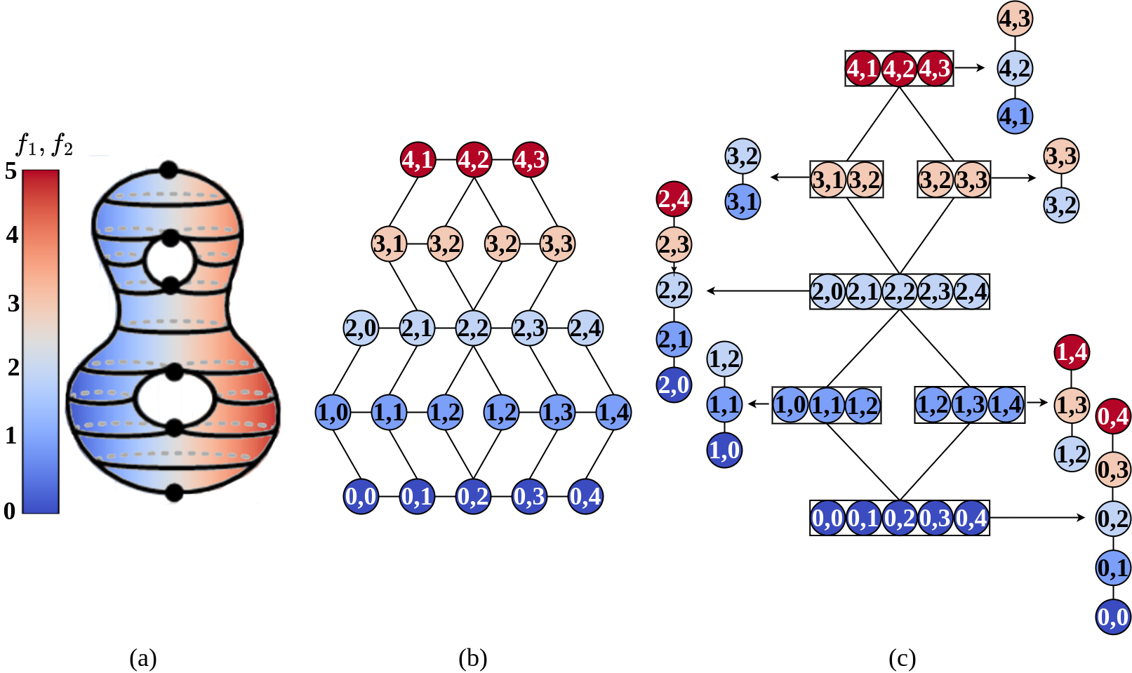
Let be a triangulated mesh of a compact -manifold . A multi-field on with component scalar fields is defined as a continuous map . For a value , its inverse is called a fiber. Each connected component of a fiber is a fiber-component 2004-Saeki-Topology-of-Singular-Fibers ; 2014-Saeki-Visualizing-Multivariate-Data . In particular, for a scalar field , the inverse of corresponding to a point in the range is called a level set and each connected component of a level set is called a contour. The Reeb space of , denoted by , is the quotient space by contracting each fiber-component to a point 2008-Edelsbrunner-ReebSpaces . In particular, the Reeb space of a scalar field is known as the Reeb graph , which is obtained by contracting each contour to a point and is the corresponding quotient map. 2017-Saeki-Theory-of-Singular-Fibers . Carr et al.2014-Carr-JCN proposed the Joint Contour Net (JCN) data-structure, which is a quantized approximation of the Reeb space. For construction of the JCN of , the range of is subdivided into a finite set of -dimensional intervals. For each interval, the inverse of is a quantized fiber and each connected component of a quantized fiber is a quantized fiber-component or joint contour. The JCN is a graph where a node corresponds to a joint contour and an edge between two nodes corresponds to the adjacency of the corresponding joint contours in the domain.
3.2 Multi Dimensional Reeb Graph
A multi-dimensional Reeb graph (MDRG) of a multi-field , proposed by Chattopadhyay et al.2014-Chattopadhyay-ExtractingJacobiStructures ; 2016-Chattopadhyay-MultivariateTopologySimplification , is the decomposition of the Reeb space (or a JCN) into a series of Reeb graphs in different dimensions. To construct the MDRG of , the Reeb graph of the function is computed. Each point represents a contour of . For every a Reeb graph corresponding to the field is computed by restricting on . This procedure is repeated by computing the Reeb graphs for the function by restricting on the contours corresponding to points in the Reeb graphs of , where . In practice, the MDRG is constructed from a quantized approximation of the Reeb Space (JCN). Therefore, similar to the JCN, the MDRG also depends on the subdivision of the range. Each node in a Reeb graph of the MDRG corresponds to a quantized contour and the adjacency between quantized contours is represented by an edge in the Reeb graph. Figure 1 shows the JCN and MDRG corresponding to a bivariate field. In the current paper, we compute persistence diagrams corresponding to Reeb graphs in the MDRG and propose a distance to compare the collection of persistence diagrams of two MDRGs based on the bottleneck distance between Reeb graphs 2014-Bauer-DistanceBetweenReebGraphs .
3.3 Persistence Diagram
In this paper, we give a brief introduction to the notion of persistence diagrams and refer the readers to 2010-Edelsbrunner-book ; 2007-Zomorodian-ComputingPersistentHomology for further details on persistent homology.
Let be a continuous real-valued function defined on . For a value , the sublevel set consists of the points in with -value less than or equal to , i.e. . For , the -th homology groups of the sublevel sets and are connected by the inclusion map . A value is a homological critical value of if such that is not an isomorphism for all sufficiently small , where is the set of non-negative integers. We assume that is tame, i.e, the number of homological critical values of is finite and the homology groups are finite-dimensional . Here, is any homological critical value of . Let be the homological critical values of . In this paper, we consider homology with coefficients in , which is the group of integers modulo . Therefore, is a vector space for . We have the following sequence of vector spaces,
| (1) |
where the homomorphisms are induced by the inclusions . A homology class is born at if but for . Further, a class which is born at dies at if for any , but . Such birth and death events are recorded by persistent homology. The -th ordinary persistence diagram is a multiset of points in , where . Each point in the th ordinary persistence diagram corresponds to a -homology class which is born at and dies at . The multiplicity of a point with is defined in terms of the ranks of the homomorphism and the points along the diagonal have infinite multiplicity.
In general, not all homology classes die during the sequence in equation (1). Such homology classes are is said to be essential. An essential homology class of dimension is denoted by a point in the th ordinary persistence diagram, where is the critical value corresponding to the birth of the homology class. By appending a sequence of relative homology groups to equation (1), we obtain the following sequence:
| (2) |
where denotes the super-level set of , and is a relative homology group 2010-Edelsbrunner-book . Essential homology classes are created in the ordinary part and are destroyed in the relative part of the sequence in equation (2). The birth and death of essential homology classes are encoded by the extended persistence diagram. An essential homology class of dimension which is born at and dies at is denoted by the point in the th extended persistence diagram.
3.4 Bottleneck Distance between Persistence Diagrams
The bottleneck distance between persistence diagrams and is defined as follows:
| (3) |
where ranges over bijections between and . For each point in , we add its nearest diagonal point in and vice-versa. The number of points in and are now equal. To compute the bottleneck distance, a bijection is constructed such that is minimized.
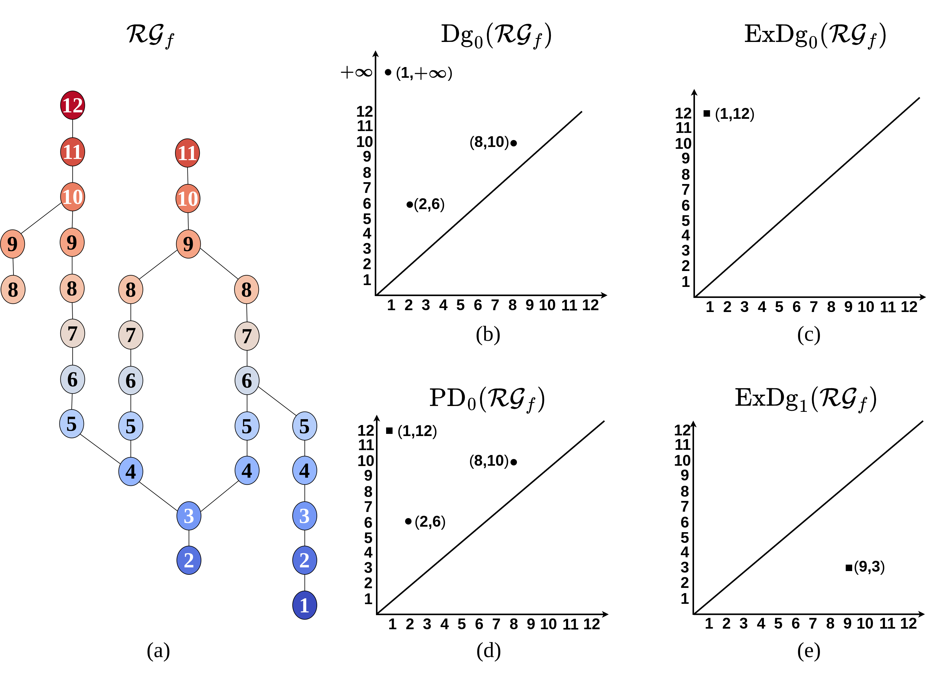
3.5 Reeb Graph and Persistence Diagram
Let be a real-valued continuous function defined on . The Reeb graph of , denoted by , is the quotient space of contours of . The function induces a real-valued function , which takes each point in to the value of corresponding to its contour in the domain, .
The persistence of topological features of are encoded in the persistence diagrams , , and . The -dimensional persistent homological features corresponding to the sub-level set and super-level set filtrations of are captured in and respectively. encodes the range of and captures the -cycles or loops in .
To compute the persistence diagrams of , we require to be the Reeb graph of a Morse function. If is a Morse function, i.e. all its critical points are non-degenerate and are at different levels, then the critical nodes of have distinct values of and belong to one of the following five-types: (i) a minimum (with down-degree , up-degree ), (ii) a maximum (with up-degree , down-degree ), (iii) a down-fork (with down-degree , up-degree ) and (iv) a up-fork (with up-degree , down-degree ). A regular node has up-degree = and down-degree . A down-fork (similarly, up-fork) node is called an essential down-fork node when it contributes to a loop (cycle) of the Reeb graph. Otherwise it is called an ordinary down-fork node. To ensure that is the Reeb graph of a Morse function, we first eliminate degenerate critical nodes in by breaking them into non-degenerate critical nodes 2019-Tu-PropogateAndPair . After eliminating degenerate critical nodes, we ensure that the critical nodes of are at different levels. If two critical nodes are at the same level, then the value of one of the nodes is increased/decreased by a small value . After removing degenerate critical nodes and ensuring that critical nodes are at different levels, becomes the Reeb graph of a Morse function.
The points in are computed by pairing ordinary down-forks with minima, ordinary up-forks with maxima and the global minimum with global maximum. Let be an ordinary down-fork of . The two lower branches of correspond to two different components and in . Let and be the global minimum of and respectively. Let us assume that . Then a -dimensional homology class is born at and dies at . is paired with and point is created in (see Figure 2(b)). A symmetric procedure is applied on to obtain points in by pairing up-forks with maxima. Let correspond to the global minimum and maximum of respectively. We pair with , giving rise to the point in (see Figure 2(c)).
We are interested in the persistent features which are born and die within the range of . In Figure 2(b), the point corresponds to the unique homology class born at the global minimum of and persists throughout the sub-level set filtration. However, the point encodes both the minimum and maximum of (see Figure 2(c)). Therefore, is combined with to obtain . This persistence diagram consists of the points in except the point with infinite persistence , instead the point in is included. Thus (see Figure 2(d)).
To compute the points in the st extended persistence diagram , we pair essential down-forks with essential up-forks. Let be an essential down-fork of . Of all the cycles born at , let be a cycle having the largest minimum value of . Let be the node corresponding to the minimum on . It can be seen that is an essential up-fork 2006-Agarwal-ExtremeElevation . is paired with giving rise to the point in (see Figure 2(e)). In this paper, we compute the persistence diagrams and of the Reeb graphs in an MDRG.
Next, we provide a brief description of the Laplace Beltrami operator and show its utility in computing descriptors of a shape.
3.6 Laplace Beltrami Operator
Let be a Riemannian -manifold in . For a twice-differentiable function , the Laplace Beltrami (LB) operator is defined as follows:
| (4) |
where grad is the gradient of and div is the divergence on the manifold 1984-chavel-eigenvalues . Let be a diffeormorphism from an open set to with
where the matrix is a Riemannian tensor on and is the determinant of . The LB operator can now be written as follows 1997-Rosenberg-Laplacian :
| (5) |
The Riemannian metric determines the intrinsic properties of , which are independent of the embedding of . Further, since the definition of is based on inner products which are rotation invariant, is also invariant to rotations of .
3.6.1 Discretization of the Laplace Beltrami operator
Let be a triangulation of the surface , with as the set of vertices. Two vertices in are said to be adjacent if they are connected by an edge. The set of adjacent vertices of is denoted by . The LB operator at a vertex is written as follows:
| (6) |
where, is the area of the Voronoi cell (shaded region) shown in Figure 3.
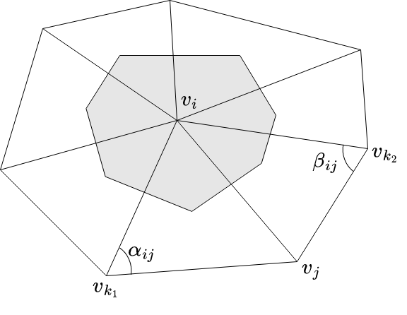
A weight function is defined as follows:
| (7) |
When is restricted to the vertices of , its discrete version is with . The discrete LB operator of is written as . The entries of the matrix are given by
The eigenvalues and eigenfunctions of the discrete version of the LB operator are computed by solving the eigenvalue problem . We note, the matrix is not symmetric since may not be the same for all vertices of . Therefore, the set of eigenvalues of this problem is not guaranteed to be real 2007-Rustamov-Laplace-Beltrami-Eigenfunctions . However, the matrix can be factorized as , where is a diagonal matrix with and is defined as follows:
| (8) |
The eigenvalue problem is rewritten as the generalized eigenvalue problem , or
| (9) |
Since the matrices and are symmetric and is positive-definite, the eigenvalues and eigenvectors are real. Further, the eigenvalues are non-negative and the eigenvectors are orthogonal in terms of -inner product:
In this paper, we obtain the feature descriptors of a shape based on the eigenfunctions of LB operator.
4 Proposed Distance between MDRGs
In this section, we propose a distance measure between shapes by defining a distance measure between two MDRGs based on the bottleneck distance between Reeb graphs 2014-Bauer-DistanceBetweenReebGraphs . First we discuss our measure for bivariate fields.
4.1 Distance between Bivariate Fields
Let be two piecewise linear bivariate fields defined on and let and be the corresponding MDRGs. To compute the proposed distance between and , we compute a sum of bottleneck distances between the component Reeb graphs in each dimension of the MDRGs by considering all possible bijections between the component Reeb graphs.
In the first dimension of the MDRGs, there is only one Reeb graph corresponding to each of the fields and , denoted by and , respectively. Let, and be the ranges of the functions and . We define as the union of the ranges of and . Now for each , in the second dimension, the MDRGs and may have multiple Reeb graphs corresponding to and restricted on and , respectively. Let be the set of Reeb graphs from the second dimension of and be the set of Reeb graphs from the second dimension of . We consider all possible bijections between and . Then we define a distance between and as follows.
| (10) |
where is a persistence diagram of the Reeb graph , ranges over bijections between and . If , then is the length of the interval , otherwise .
In the current paper, corresponding to each of the Reeb graph in an MDRG, we construct two persistence diagrams, namely and , as discussed in Section 3.5. We compute the distance between MDRGs defined in equation (LABEL:eqn:bottleneck-distance-mdrgs) based on and , which are denoted by and , respectively. We consider the proposed distance measure between and as the weighted sum of , and .
| (11) |
where, and . Here, and respectively compute the distance between persistence diagrams of sub-level set and super-level set filtrations of the Reeb graphs in the MDRGs and is the distance between the -st extended persistence diagrams of the Reeb graphs in and respectively. Next, we discuss how to compute the proposed distance measure for quantized fields.
4.1.1 Computational Aspects for Quantized Fields
We note, the MDRG of a bivariate field can be computed from the corresponding JCN, which is a quantized approximation of the Reeb space. For constructing the JCN of a bivariate field, the range of each of the component scalar fields is quantized or subdivided into a finite number of slabs. Algorithm 1 outlines the computation of the persistence diagrams by computing an MDRG corresponding to a bivariate field and quantization levels and . ConstructJCN (in line 2) computes the JCN of corresponding to and . ConstructMDRG (in line ) constructs the MDRG from the JCN. Finally, ComputePDReebGraph computes the persistence diagram corresponding to a component Reeb graph (lines -).
Input:
Output: Persistence diagrams of the component Reeb graphs in the MDRG
Algorithm 2 gives the pseudo-code for computing the distance between two multi-fields using the proposed distance measure. Let and be two bivariate fields defined on a compact -manifold with . Let and be the number of slabs (quantization levels) into which and are subdivided respectively, for constructing the JCNs of and . Then let be the quantized range values corresponding to the subdivision of . The distance between MDRGs defined in equation (LABEL:eqn:bottleneck-distance-mdrgs) can be written as:
| (12) |
where ranges over all possible bijections between and . Since the number of Reeb graphs in and need not be equal, it may not be possible to construct proper bijections between and . Therefore, we introduce dummy Reeb graphs (without vertices and edges) in or to make the cardinality of and equal. Then the optimal bijection is constructed using the Hungarian algorithm by computing a cost matrix 1955-Kuhn-Hungarian-Algorithm (lines - of Algorithm 2). We note, the bijection can map a Reeb graph in to a dummy Reeb graph. The persistence diagram corresponding to a dummy Reeb graph is empty, i.e, it does not contain any point. The bottleneck distance between persistence diagrams is computed as described in Section 3.4.
Input:
Output:
4.2 Properties of the Proposed Distance Measure
In this sub-section, we discuss the properties of the proposed distance between MDRGs. Let be two bivariate fields. First, we show that is a pseudo-metric.
Theorem 4.1
satisfies the properties of a pseudo-metric.
Proof
Non-negativity: For two MDRGs and , we have . Thus the non-negativity property is satisfied.
Symmetry: For two MDRGs and , we have . Thus the symmetry property holds.
Identity: Bauer 2014-Bauer-DistanceBetweenReebGraphs showed that two distinct Reeb graphs can have the same persistence diagram and therefore the bottleneck distance between Reeb graphs is a pseudo-metric. Since we compute by calculating the bottleneck distance between the component Reeb graphs of the MDRGs and , it follows that the bottleneck distance between two non-identical MDRGs and can be zero. Therefore, the identity property does not hold.
Triangle inequality: Let us consider three MDRGs and , corresponding to bivariate fields and , respectively. We first prove the triangle inequality property for between MDRGs. We need to show that .
For , let be the bijection between and achieving . Similarly, let be the bijection between and achieving . Let be the bijection between and obtained by the composition of and , i.e, .
| (since between Reeb graphs is a pseudo-metric) | ||
Using a similar argument, we can prove the triangle inequality for . We now show the triangle inequality property for .
Next, we prove the stability of the proposed measure . Let and be two bivariate fields defined on a compact metric space such that and are tame functions. Let and be the MDRGs of and , respectively. Then we prove the following lemma.
Lemma 1
where denotes the amplitude of a real-valued function and is defined as follows:
Proof
The term in of equation () is bounded above by (see 2007-Cohen-Steiner-Bottleneck for more details). We now prove a bound on the term .
Let . Now, every point in the persistence diagram corresponds to a -dimensional class whose birth and death lies between and . Therefore, the maximum persistence of a point in is at most the amplitude of in .
| (13) |
Similarly, for , the following bound is obtained on the maximum persistence of a point in the persistence diagram .
| (14) |
Let and be its matching pair in corresponding to . Then is at most . Otherwise, we can match to , to and obtain the required bound. Therefore, for any matched pair of points , is bounded by . We now obtain a bound on as follows:
Lemma 2
Proof
The term in is bounded above by (see Theorems and in 2014-Bauer-DistanceBetweenReebGraphs for more details). The rest of the proof is similar to that of Lemma 1.
The following theorem gives the stability of .
Theorem 4.2
Stability:
4.3 Complexity Analysis
In this sub-section, we analyze the time and space complexities of computing the distance between two bivariate fields based on the corresponding MDRGs. First, we give the complexity for constructing the MDRG of a bivariate field and computing the persistence diagrams of the component Reeb graphs of the MDRG. Then, we analyze the complexity of computing the proposed distance measure between two MDRGs.
4.3.1 Algorithm 1: Computing the MDRG and Persistence Diagrams of its Component Reeb Graphs
Time Complexity. Let be a bivariate field defined on a compact -manifold. To construct the MDRG of , denoted by , we require a JCN as input. The construction of the JCN takes time, where is the number of edges in the JCN and is the inverse Ackermann function 1975-Tarjan-UF (line , Algorithm 1). The time complexity of constructing the MDRG from the JCN using the algorithm in 2016-Chattopadhyay-MultivariateTopologySimplification is , where is the number of vertices of the JCN (line , Algorithm 1). We note, the Reeb graph has at most vertices and edges. Therefore, has at most simplices (vertices and edges). The computation of the persistence diagram of take time 2010-Edelsbrunner-book (line , Algorithm 1). Next, we see the time complexity of computing the persistence diagrams of the Reeb graphs of in (lines -, Algorithm 1).
We note, each node/edge in a Reeb graph () corresponds to a unique node/edge in the JCN 2016-Chattopadhyay-MultivariateTopologySimplification . Therefore, the total number of simplices (vertices and edges) in the second-dimensional Reeb graphs of is at most the total number of simplices in the JCN. Thus, the construction of the persistence diagrams of the Reeb graphs of , i.e. take time. The total time for constructing the MDRG of and computing the persistence diagrams of its component Reeb graphs (in Algorithm 1) is . Next, we analyze the space complexity of computing and persistence diagrams of the Reeb graphs in .
Space Complexity. The space complexity of constructing the JCN of depends on the number of edges it contains and the number of fragments in the domain corresponding to the quantization of , denoted by . Since 2014-Carr-JCN , the space complexity of computing the JCN is . The number of nodes/edges in is bounded by the number of nodes/edges in the JCN. Thus the Reeb graph takes space. Similarly, based on the bound obtained on the number of simplices in the Reeb graphs , the Reeb graphs in the second dimension of take space. Thus, the space complexity of is . Next, we analyze the space complexity for the persistence diagrams of the Reeb graphs in . We note, the persistence diagram of a Reeb graph is obtained by pairing its critical nodes. Therefore, the number of points in a persistence diagram is at most half the number of vertices in the corresponding Reeb graph. The total number of nodes in the component Reeb graphs of is at most . Thus, the total number of points in the persistence diagrams of the Reeb graphs in is . The total space complexity of computing and the persistence diagrams of its component Reeb graphs is .
4.3.2 Algorithm 2: Computing the Distance between MDRGs
Time Complexity. Let be two bivariate fields and be the corresponding MDRGs. Let and be the number of vertices and edges in the JCNs of and respectively. Then the total number of points in the persistence diagrams of the component Reeb graphs of and are at most and respectively (see Section 4.3.1 for more details). Therefore, the total time for computing and using the Hungarian algorithm is 1955-Kuhn-Hungarian-Algorithm .
Let be the number of slabs into which is subdivided, for constructing the JCNs of and . Then let be the quantized range values corresponding to the subdivision of . For each , we need to compute a map which achieves the minimal value of (lines -, Algorithm 2). To do so, we need to compute for each and . The total time for computing is bounded by the time complexity for computing the bottleneck distance between all pairs of Reeb graphs in the second dimension of and , which is . After this step, the computation of all the optimal bijections using Hungarian algorithm take time 1955-Kuhn-Hungarian-Algorithm . The total time for computing the distance between the collections of persistence diagrams of and (in Algorithm 2) is . Next, we analyze the space complexity of the proposed distance between MDRGs.
Space Complexity. The distance between and is computed based on the bottleneck distance between the persistence diagrams of the component Reeb graphs in the respective MDRGs. To compute the bottleneck distance between the persistence diagrams of two Reeb graphs, we construct an optimal bijection between the points in the persistence diagrams using the Hungarian algorithm. For two persistence diagrams consisting of and points respectively, the Hungarian algorithm takes space. Based on the bound obtained on the number of points in the persistence diagrams of and , the space complexity for computing is . Similarly, the total space complexity for the computation of for all combinations of and , is . Thus the computation of distance between MDRGs takes space.
4.4 Generalization for more than two fields
Although, in this paper, we deal with MDRGs of bivariate fields, the proposed distance measure can be extended for MDRGs corresponding to more than fields. If and are multi-fields defined on a triangulated mesh of dimension , then the distance between the MDRGs and is defined as follows:
| (15) |
Here, and denote the collections of Reeb graphs in the dimension of and respectively, varies over bijections between and , and represents the union of the ranges of and . Similar to the case of bivariate fields, we denote the distance between MDRGs based on the persistence diagrams and by and , respectively. We now define a distance between and as follows.
| (16) |
where, and . Here, and respectively compute the distance between persistence diagrams of sub-level set and super-level set filtrations of the Reeb graphs in the MDRGs and is the distance between the -st extended persistence diagrams of the Reeb graphs in and respectively. We note, is a pseudo-metric.
Theorem 4.3
satisfies the properties of a pseudo-metric.
The proof of this theorem is similar to that of Theorem 4.1. Next, we show the stability of .
Theorem 4.4
Stability:
The bound on consists of two terms. The proof of the first and second terms are similar to the proofs of Lemmas 1 and 2 respectively.
Next, we show the experimental results of the proposed method on two datasets.
5 Experimental Results
In this section, we show the application of the proposed distance measure in shape matching and detecting topological features in a time varying multi-field data.
5.1 Classification and Analysis of Shape Data
In this subsection, we show the effectiveness of the proposed distance between MDRGs in matching shapes. First, we describe the feature descriptors corresponding to a shape for computing the MDRGs.
5.1.1 Feature Descriptors of a Shape
We obtain scalar fields based on the eigenfunctions of discrete Laplace-Beltrami operator (see equation (9)) for computing the MDRG. The eigenvalues s of the discrete LB operator are sorted in the non-decreasing order. The first eigenvalue is zero and the corresponding eigenfunctions are constant 2006-Reuter-Shape-DNA . Therefore, we consider the eigenvalues for . The ability of the eigenfunctions in capturing the geometric and topological properties of a shape and their invariance to isometry of shapes 2006-Levy-Laplace-Beltrami-Eigenfunctions ; 2007-Rustamov-Laplace-Beltrami-Eigenfunctions make them suitable shape descriptors.
To remove the effect of scale, each eigenfunction is normalized by its corresponding eigenvalue 2007-Rustamov-Laplace-Beltrami-Eigenfunctions . For a triangulated shape with vertices , the normalized eigenfunction corresponding to eigenvalue is an -dimensional vector , where is the value of the eigenfunction at the vertex .
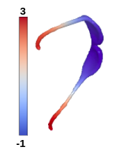
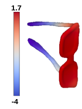
Sign Ambiguity Problem: We now encounter the sign ambiguity problem while dealing with the eigenfunctions of the LB operator. If is an eigenfunction corresponding to the eigenvalue , then is also an eigenfunction for . We have to pick one among them as the eigenfunction for . If we arbitrarily choose either of or , then there is a possibility of two similar shapes having eigenfunctions which are negative of each other (See Figure 4). Therefore, for each eigenvalue , we need to systematically pick one of or . This is known as the sign ambiguity problem 2007-mateus-shape-matching , for which Umeyama 1988-Umeyama-EigenDecomposition proposed a solution by taking the absolute values of eigenfunctions. In this paper, we adopt this solution and choose the functions as shape descriptors.
We show the effectiveness of using absolute values of eigenfunctions as feature descriptors with respect to HKS 2009-Sun-HKS , WKS 2011-Aubry-WKS and SIHKS 2010-Bronstein-SIHKS . The descriptors HKS and SIHKS depend on the number of time parameters 2009-Sun-HKS ; 2010-Bronstein-SIHKS and WKS depends on the number of energy distributions 2011-Aubry-WKS . Following 2014-Li-Persistence-Based-Structural-Recognition , we have fixed the number of time parameters as for HKS, for SIHKS, and the number of energy distributions as for WKS. The number of eigenfunctions is chosen as for constructing HKS, WKS and SIHKS. The distance between two shapes with respect to a distance measure is defined as the sum of distances computed at each time (for HKS, SIHKS) or energy distribution (for WKS). For example, the distance between shapes and using HKS is given by:
| (17) |
where is the distance measure and is the HKS at time .
5.1.2 SHREC Dataset
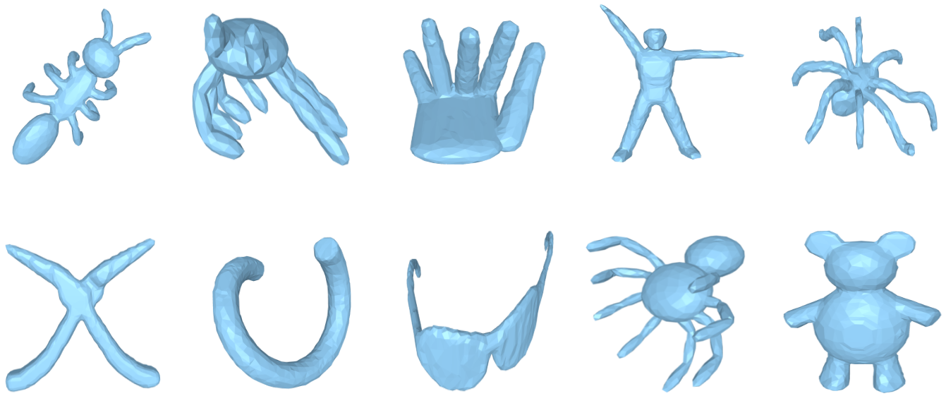
We show the experimental results of the proposed measure in the Shape Retrieval Contest (SHREC) dataset and compare the results with various topological distance measures in the literature. The SHREC dataset 2010-SHREC consists of watertight shapes classified into categories. A sample of the shapes are shown in Figure 5. Each of the meshes is simplified into faces 2014-Li-Persistence-Based-Structural-Recognition . We compare the performance of the proposed distance between MDRGs with the distance between MRSs 2021-Ramamurthi-MRS and the distance between histograms corresponding to fiber-component distributions 2019-Agarwal-histogram . We evaluate the efficiency of distance measures by the standard evaluation techniques NN, FT, ST, E-measure, and DCG (see 2010-SHREC for details). These techniques take a distance matrix consisting of distances between all pairs of shapes and return a value between and , where higher values indicate better efficiency.
We first show the significance of bivariate fields over scalar fields using the proposed distance measure . Table 1 shows the results of between MDRGs using a pair of eigenfunctions (bivariate field) and the bottleneck distance between Reeb graphs using individual eigenfunctions (scalar field). The bivariate field using MDRG produces a better result than the Reeb graphs of the individual scalar fields, thereby indicating its significance.
| Descriptor | NN | -Tier | -Tier | e-Measure | DCG |
|---|---|---|---|---|---|
The efficiency in computing the distance between shapes will be higher when the shapes are compared based on many eigenfunctions. However, a D shape is a -dimensional manifold. If more than fields are applied on a shape, then the corresponding Reeb space is not defined. Therefore, we generalize the distance between shapes and for more than two eigenfunctions as follows.
| (18) |
where is the number of eigenfunctions and is the MDRG for the shape with and as the component scalar fields. Table 2 shows the performance of the proposed method for varying number of eigenfunctions. The results clearly indicate the increase in efficiency with increase in the number of eigenfunctions.
| NN | -Tier | -Tier | e-Measure | DCG | |
|---|---|---|---|---|---|
Table 3 shows the performance of HKS, WKS, SIHKS and absolute values of eigenfunctions as shape descriptors for various distance measures. The distance measures for HKS, WKS and SIHKS are computed using equation (17). We set the parameters for various distance measures as follows. The distance between MDRGs is computed as specified in equation (18), where and the weights and are set equally. The number of slabs for constructing the JCNs (required for computing MDRGs) is , the parameters and for the distance between fiber-component distributions are set to and the MRSs are constructed for resolutions.
| Descriptors | Methods | NN | -Tier | -Tier | e-Measure | DCG |
|---|---|---|---|---|---|---|
| HKS | Histogram | |||||
| MRS | ||||||
| of Reeb graph | ||||||
| WKS | Histogram | |||||
| MRS | ||||||
| of Reeb graph | ||||||
| SIHKS | Histogram | |||||
| MRS | ||||||
| of Reeb graph | ||||||
| Pairs of Eigen-functions | Histogram | |||||
| MRS | ||||||
| s of MDRG |
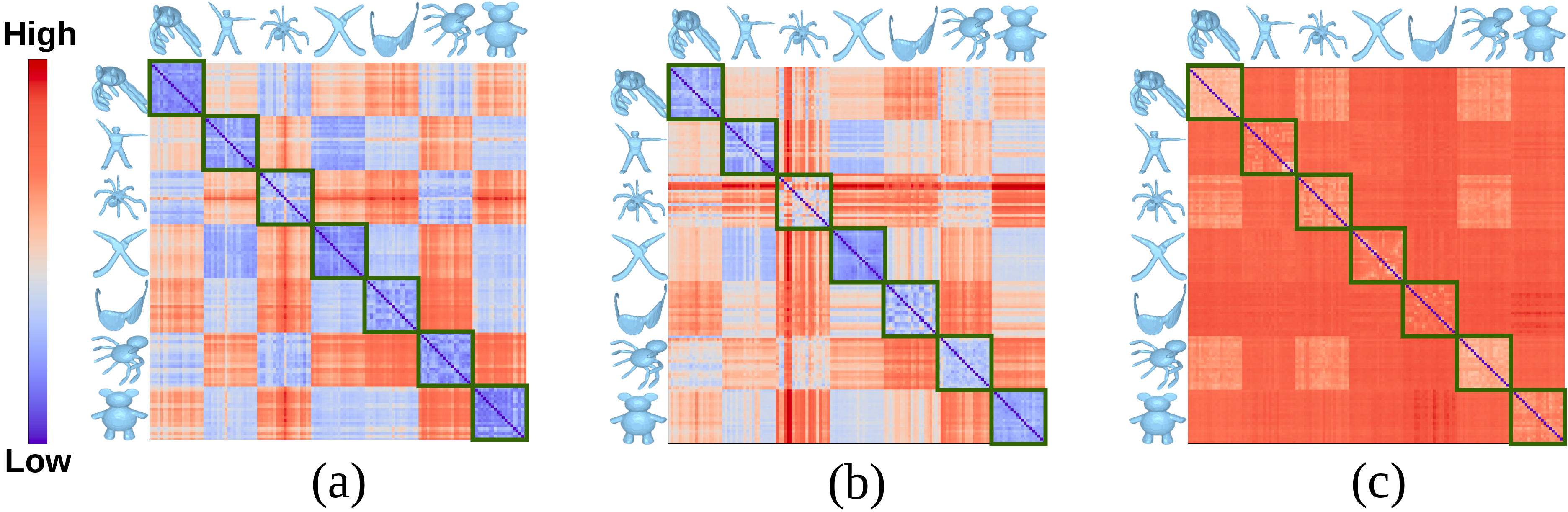
From the table, it can be seen that MDRG using eigenfunctions produces better results than HKS and WKS (for all the methods). With eigenfunctions as shape descriptors, the proposed method performs better than the histogram of fiber-component distributions and the results are comparable with that of MRS. On the other hand, the bottleneck distance between Reeb graphs outperforms other methods using SIHKS. However, the proposed measure using eigenfunctions performs better than the bottleneck distance between Reeb graphs using SIHKS when we experiment with categories of shapes, which can be observed in the distance matrices in Figure 7.
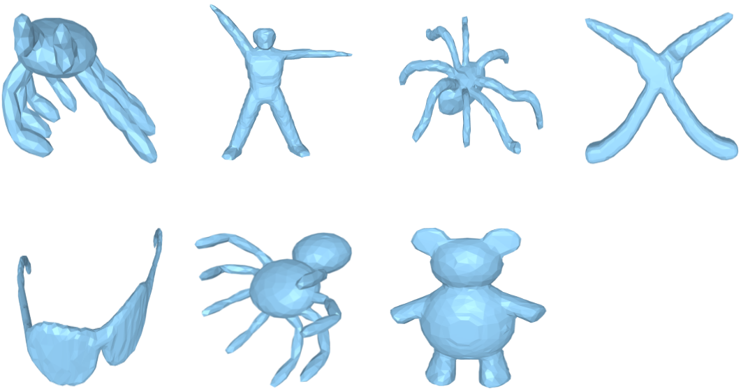
5.1.3 Results for Seven Categories of Shapes
We experiment with of the categories of shapes shown in Figure 6 and the results are provided in Table 4. Similar to the results in Table 3, MDRG using eigenfunctions performs better than other techniques using HKS and WKS. Further, the results of the distance between MDRGs are comparable with that of MRSs using eigenfunctions and the bottleneck distance between Reeb graphs using SIHKS. This can be seen from the distance matrices shown in Figure 7. The proposed distance using MDRGs is better in discriminating different classes of shapes as compared to the distances based on Reeb graphs and MRSs.
| Descriptors | Methods | NN | -Tier | -Tier | e-Measure | DCG |
|---|---|---|---|---|---|---|
| HKS | Histogram | |||||
| MRS | ||||||
| of Reeb graph | ||||||
| WKS | Histogram | |||||
| MRS | ||||||
| of Reeb graph | ||||||
| SIHKS | Histogram | |||||
| MRS | ||||||
| of Reeb graph | ||||||
| Pairs of Eigen-functions | Histogram | |||||
| MRS | ||||||
| s of MDRG |
5.1.4 Classification Results
We measure the effectiveness of the proposed method in the classification of the shapes by performing a -fold cross-validation using a decision tree classifier. The dataset is randomly divided into folds. The cross-validation is performed for iterations. In each iteration, one of the folds is taken as the test set and the rest of the folds constitute the training set. For each shape , we consider a feature vector, which consists of the distances from to every shape in the dataset. The classifier is trained based on the feature vectors of the shapes in the training set. The category of a shape in the test set is determined by the classifier based on its feature vector.
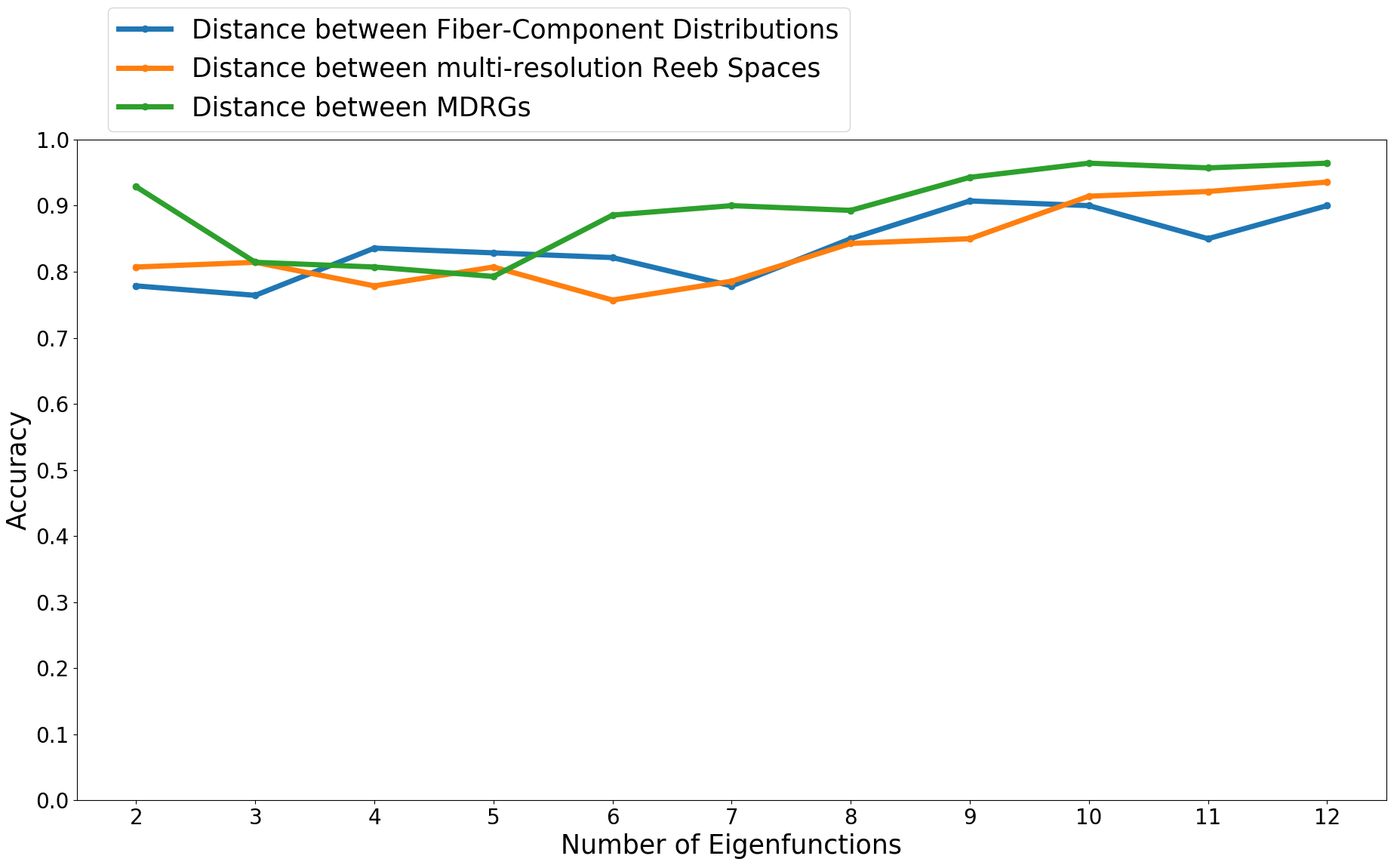
We perform the experiments with categories of shapes, described in Section 5.1.3. Figure 8 shows the classification accuracy results using three different distances based on multi-field topology, viz., (i) the distance between histograms of fiber-component distributions 2019-Agarwal-histogram , (ii) the distance between MRSs 2021-Ramamurthi-MRS and (iii) the proposed distance between MDRGs, using pairs of eigenfunctions as the shape descriptor (as in Section 5.1.2). The accuracies are plotted for varying numbers of eigenfunctions. From the plots, we observe that the classification accuracy is higher for more eigenfunctions. Further, the proposed distance gives the best accuracy when we use eigenfunctions as the shape descriptor.
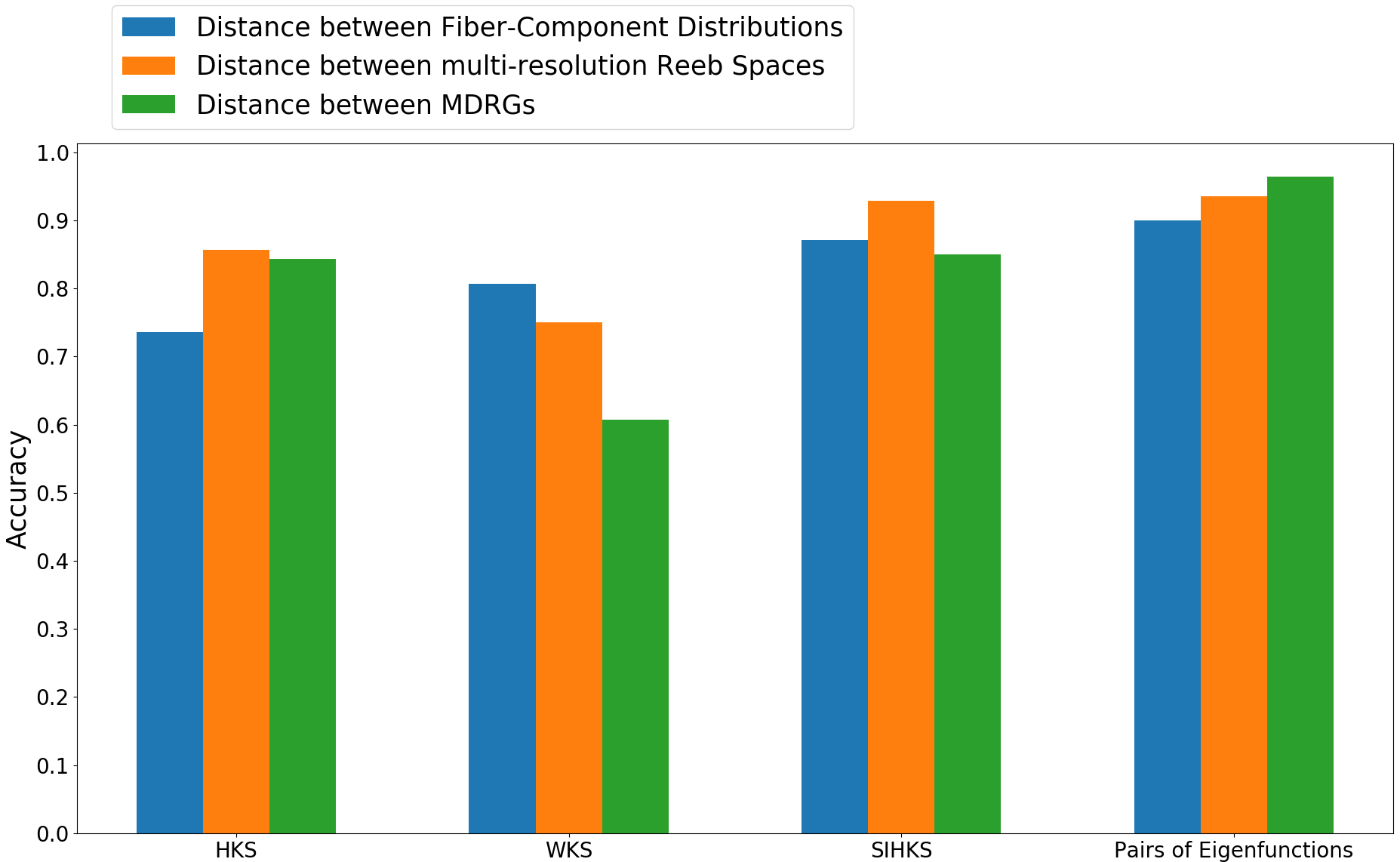
We also evaluate the classification accuracy of the same distances using HKS, WKS, SIHKS, and pairs of eigenfunctions, respectively, as shape descriptors. The results are illustrated in Figure 9. We observe that the eigenfunctions demonstrate a better ability in classifying shapes compared to HKS, WKS, and SIHKS. Further, upon using eigenfunctions as the shape descriptor, the proposed distance between MDRGs shows improved performance over other distances and feature descriptors.
Next, we show the effectiveness of the proposed distance measure in detecting topological features in a time-varying multi-field data from computational chemistry.
5.2 Classification and Analysis of Chemistry Data
Adsorption is a process where the molecules of a gas adhere to a metal surface. This phenomenon has various applications including corrosion, electrochemistry, molecular electronics and hetrogeneous catalysis 2010-kendrick-elucidating ; 2010-somorjai-introduction . In particular, the adsorption of the Carbon Monoxide (CO) molecule on the Platinum (Pt) surface has gained interest due to its industrial applications in the areas of automobile emission, fuel cells, and other catalytic processes 2009-dimakis-attraction ; 2018-patra-surface . Hence, the interaction between the CO molecule and the platinum surface at the atomic level is studied with utmost importance.
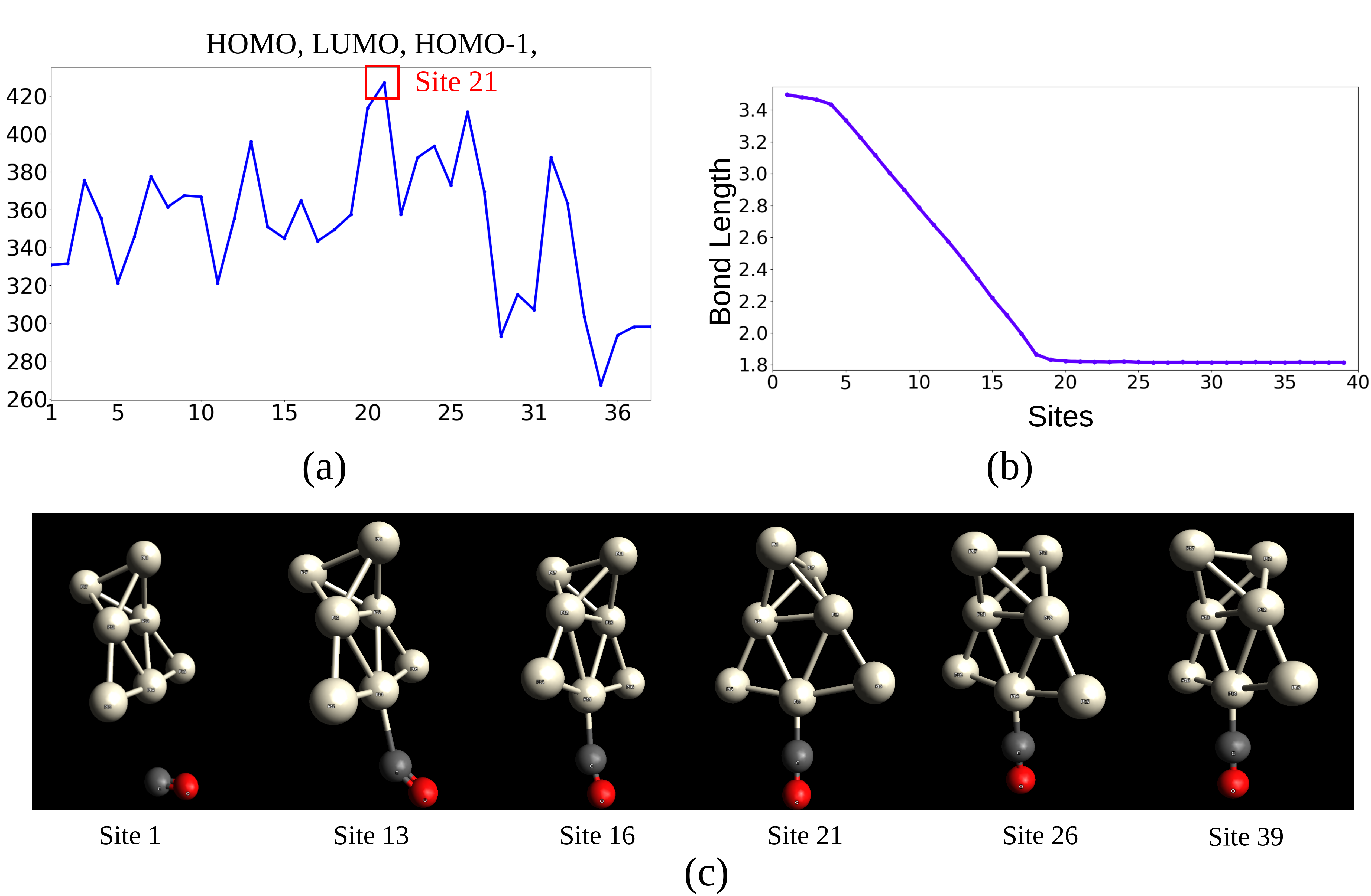
In this study, we validate the proposed method by studying the interaction of the CO molecule with a Pt7 cluster. When the CO molecule approaches the Pt7 cluster, the internal CO bond weakens and a bond is formed between one of the Pt atoms and the C atom of the CO molecule 2009-dimakis-attraction . The Pt-CO bond is formed at site , which is validated by the geometry in Figure 10(b). However, the bond length is unstable at this site. The bond stabilizes at site when the bond length between Pt and C atoms is Å(see the plot in Figure 10(c)). In this experiment, we aim to capture the stable bond formation between the Pt7 cluster and the CO molecule.
The Pt-CO dataset consists of electron density distributions generated by quantum mechanical computations corresponding to the HOMO (Highest Occupied Molecular Orbital), LUMO (Lowest Unoccupied Molecular Orbital) and HOMO-, defined on a regular grid. The orbital numbers and correspond to HOMO-, HOMO and LUMO respectively. At a series of sites, the electron density distributions are computed for varying distances between the C atom of the CO molecule and the Pt surface 2019-Agarwal-histogram .
5.2.1 Feature Detection Results
We examine the performance of the proposed measure in detecting the formation of a stable Pt-CO bond for various combinations of the orbital densities at HOMO, LUMO and HOMO- molecular orbitals. We compare the performance of scalar, bivariate and trivariate fields. In our experiments, we subdivide the range of each of the fields into slabs for constructing the JCNs. Figure 10(a) shows the plots for the trivariate field (HOMO, LUMO, HOMO-), consisting of all three scalar fields. We observe the most significant peak at site . This corresponds to the stable bond formation between Pt and C atoms, which is indicated by the bond length between Pt and C remaining constant after site (see Figure 10(b)). Ramamurthi et al.2021-Ramamurthi-MRS identified this site of the stable bond formation using the trivariate field.
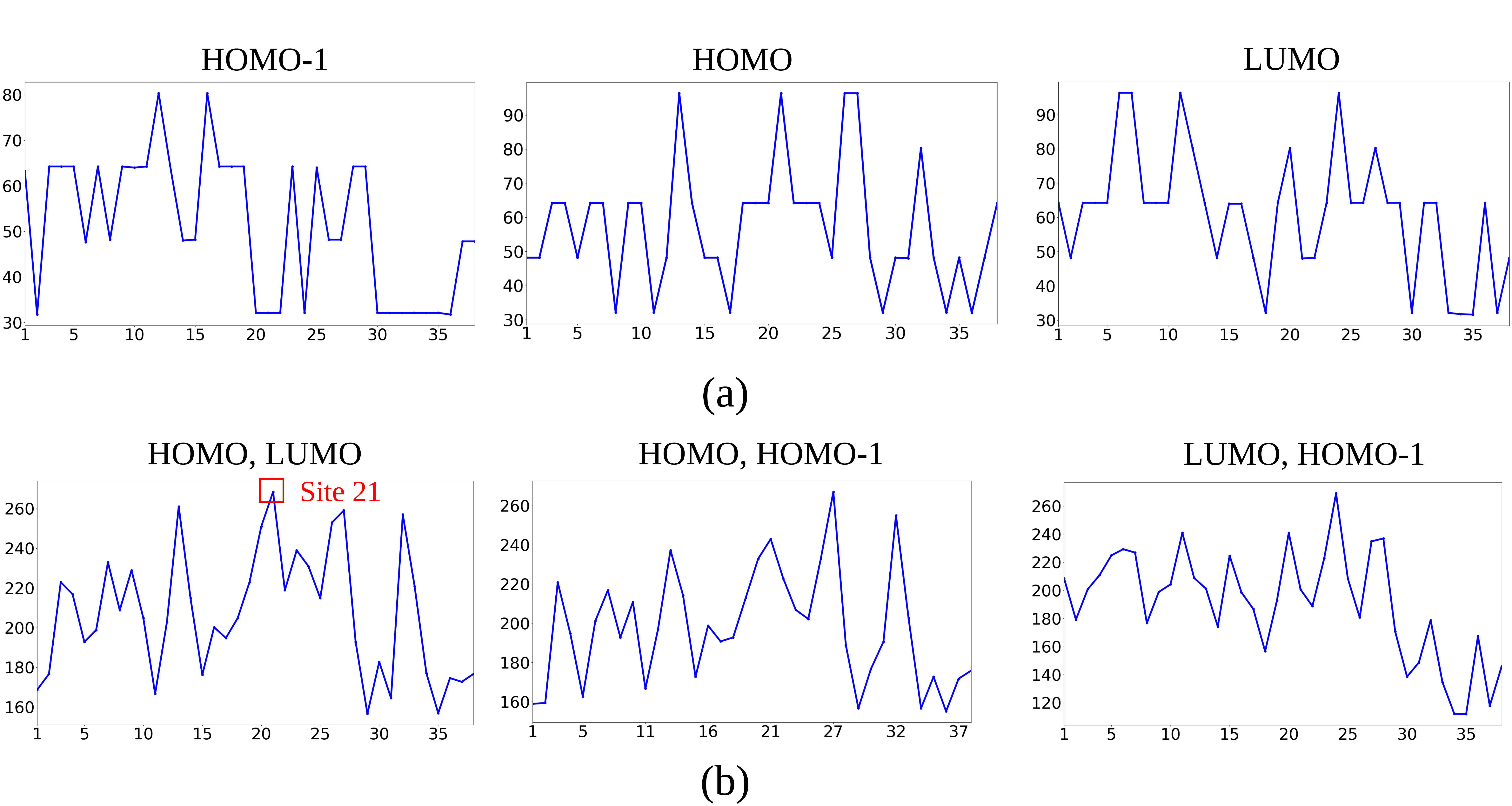
We also measure the performance of the proposed method with scalar fields and bivariate fields. Figure 11(a) shows the plots for each of the scalar fields HOMO, HOMO- and LUMO. We observe that the site of stable bond formation is not detected using each of the scalar fields. Figure 11(b) shows the plots for the bivariate fields (HOMO, LUMO), (HOMO, HOMO-) and (LUMO, HOMO-). We observe that the combinations (HOMO, HOMO-) and (LUMO, HOMO-) are unable to detect the correct site in the plots. However, for the combination (HOMO, LUMO), the site corresponding to the stable bond formation is detected, which is also observed in 2019-Agarwal-histogram ; 2021-Ramamurthi-MRS . This illustrates the significance of using multi-fields in detecting the bond formation between Pt and C atoms.
| Dataset | Shapes/Sites | Field(s) | Slabs | ||||
| SHREC | Human, Hand | s | s | s | |||
| SHREC | Human, Hand | s | s | s | |||
| SHREC | Human, Hand | s | s | s | |||
| Pt-CO | HOMO | s | s | ||||
| Pt-CO | HOMO, LUMO | s | s | ||||
| Pt-CO | HOMO, LUMO, HOMO- | s | s |
5.2.2 Classification Results
In this subsection, we evaluate the ability of the proposed distance between MDRGs in classifying a site as occurring before and after the stabilization of the bond between Pt and CO. We divide the dataset into two classes, consisting of the sites before (sites -) and after the stabilization of the Pt-CO bond (sites -), respectively. Similar to Section 5.1.4, we employ a decision tree classifier and analyze the effectiveness of methods by performing -fold cross-validation. We measure the classification accuracies and plot the Receiver Operator Characteristics (ROC) curves. The ROC curve is constructed by plotting the true positive rate of classification (TPR) against the false positive rate of classification (FPR). Here, the negative and positive classes are the sites before and after the bond stabilization, respectively. TPR (FPR) gives the proportion of the correct (wrong) predictions in the positive (negative) class. An ROC curve having a higher area under the curve (AUC) indicates better distinguishing ability between the classes.
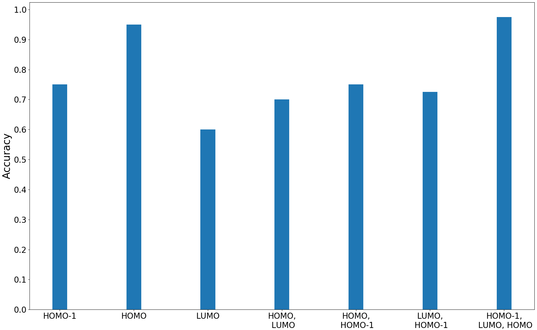
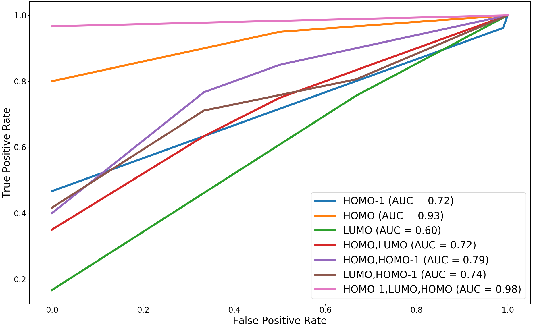
Figure 12 shows the results of classification accuracies and plots of the ROC curves for the proposed method using various combinations of HOMO, HOMO- and LUMO fields. Here, the ROC curve is computed as the mean of the ROC curves obtained for each of the folds used as a test set, in the -fold cross-validation. We observe that the distance between MDRGs using the trivariate field (HOMO-, LUMO, HOMO) obtains a better accuracy and has a higher area under the curve (AUC) compared to other field combinations.
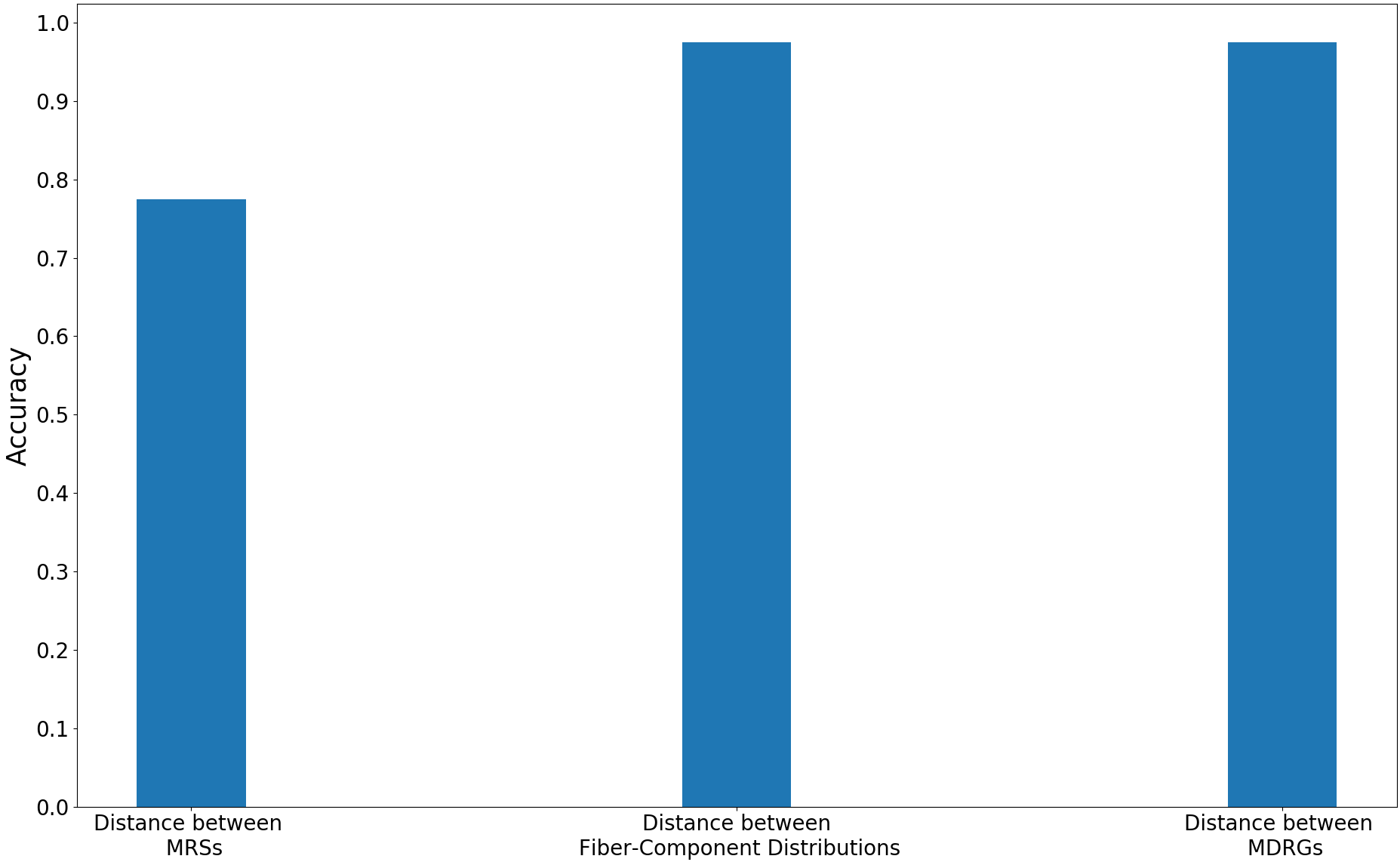
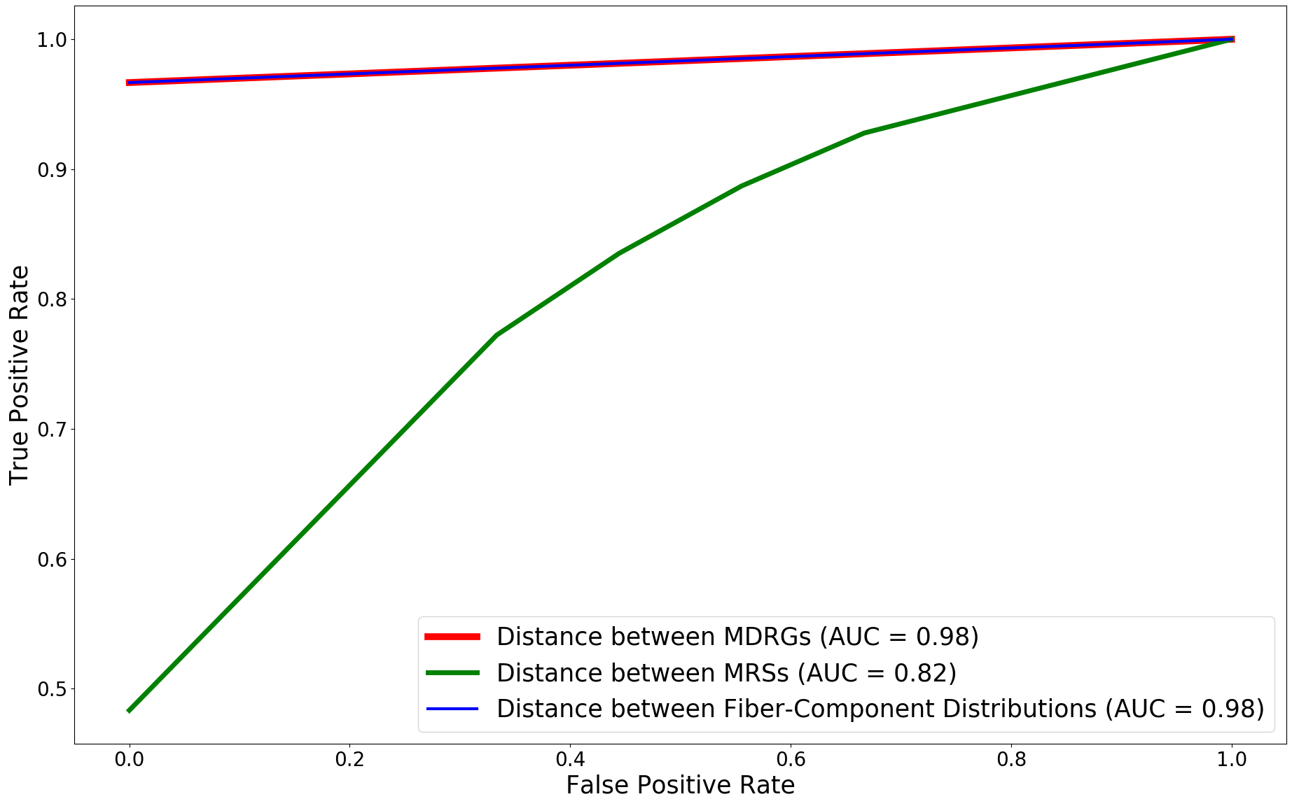
We compare the performance of the proposed method with other multi-field based distances by plotting the classification accuracies and ROC curves for the trivariate field (HOMO-, LUMO, HOMO). The plots are shown in Figure 13. The proposed method performs better than the distance between MRSs 2021-Ramamurthi-MRS and its performance is on par with the distance between fiber-component distributions 2019-Agarwal-histogram .
5.3 Computational Performance
Table 5 shows the computational performance results of the proposed distance between MDRGs in shape matching (SHREC ) and Pt-CO bond detection datasets using scalar and multi-fields. All timings were performed on a GHz -Core Intel Xeon(R) with GB memory, running Ubuntu . From the table, we observe the time taken for computing the distance between MDRGs based on the th ordinary and st extended persistence diagrams respectively.
6 Conclusion
In this article, we introduce a novel distance measure between MDRGs by computing the bottleneck distances between their component Reeb graphs. We show that the proposed distance measure is a pseudo-metric and satisfies the stability property. The effectiveness of the proposed distance measure is shown in the problem of shape classification, where the performance of using absolute values of eigenfunctions as shape descriptors is compared with HKS, WKS and SIHKS. Further, we have shown the performance of the proposed distance measure in detecting the formation of a stable bond between Pt and CO molecules. The ability of the distance is demonstrated in the classification of sites based on their occurrence before and after the stabilization of the Pt-CO bond.
The computation of the MDRG of a multi-field requires a JCN, which is computationally expensive to construct. Thus, there is a need for a faster algorithm for constructing the MDRG. We have shown applications of the proposed method in the problem of shape retrieval and in detecting the formation of a stable Pt-CO bond, which is an application in the field of computational chemistry. However, exploring other computational domains will be useful for further analysis on the effectiveness of the proposed distance measure. Further, we note, the multiplicity of the eigenvalues of the Laplace Beltrami operator can be greater than , i.e. there can be more than one eigenfunction corresponding to an eigenvalue. In such cases, there is an ambiguity in ordering the eigenfunctions according to eigenvalues. Such issues need to be addressed in the future.
7 Declarations
Funding: The authors would like to thank the Science and Engineering Research Board (SERB), India (SERB/CRG/2018/000702) and International Institute of Information Technology (IIITB), Bangalore for funding this project and for generous travel support.
Conflicts of interest:
The authors of this paper have no conflicts of interest.
Data availability statement: The datasets analysed during the current study are available from the corresponding author on reasonable request.
References
- (1) Agarwal, P., Edelsbrunner, H., Harer, J., Wang, Y.: Extreme elevation on a 2-manifold. Discrete Computational Geometry 36, 553–572 (2006). DOI 10.1007/s00454-006-1265-8
- (2) Agarwal, T., Chattopadhyay, A., Natarajan, V.: Topological Feature Search in Time-Varying Multifield Data. TopoInVis 2019, Nyköping, Sweden, preprint arXiv:1911.00687 (2019)
- (3) Aubry, M., Schlickewei, U., Cremers, D.: The wave kernel signature: A quantum mechanical approach to shape analysis. pp. 1626–1633 (2011). DOI 10.1109/ICCVW.2011.6130444
- (4) Bauer, U., Ge, X., Wang, Y.: Measuring distance between reeb graphs. In: Proceedings of the Thirtieth Annual Symposium on Computational Geometry, SOCG’14, p. 464–473. Association for Computing Machinery, New York, NY, USA (2014)
- (5) Bronstein, M., Kokkinos, I.: Scale-invariant heat kernel signatures for non-rigid shape recognition. 2010 IEEE Computer Society Conference on Computer Vision and Pattern Recognition pp. 1704–1711 (2010)
- (6) Carr, H., Duke, D.: Joint Contour Nets. IEEE Transactions on Visualization and Computer Graphics 20(8), 1100–1113 (2014). DOI 10.1109/TVCG.2013.269
- (7) Chattopadhyay, A., Carr, H., Duke, D., Geng, Z.: Extracting Jacobi Structures in Reeb Spaces. In: N. Elmqvist, M. Hlawitschka, J. Kennedy (eds.) EuroVis - Short Papers, pp. 1–4. The Eurographics Association (2014). DOI 10.2312/eurovisshort.20141156
- (8) Chattopadhyay, A., Carr, H., Duke, D., Geng, Z., Saeki, O.: Multivariate topology simplification. Computational Geometry: Theory and Applications 58, 1–24 (2016). DOI 10.1016/j.comgeo.2016.05.006
- (9) Chavel, I.: Eigenvalues in Riemannian geometry. Academic press (1984)
- (10) Chazal, F., Cohen-Steiner, D., Glisse, M., Guibas, L.J., Oudot, S.Y.: Proximity of persistence modules and their diagrams. In: Proceedings of the Twenty-Fifth Annual Symposium on Computational Geometry, SCG ’09, p. 237–246. Association for Computing Machinery, New York, NY, USA (2009). DOI 10.1145/1542362.1542407. URL https://doi.org/10.1145/1542362.1542407
- (11) Cohen-Steiner, D., Edelsbrunner, H., Harer, J.: Stability of persistence diagrams. Discret. Comput. Geom. 37(1), 103–120 (2007)
- (12) Dey, T.K., Mémoli, F., Wang, Y.: Multiscale mapper: Topological summarization via codomain covers. In: Proceedings of the Twenty-Seventh Annual ACM-SIAM Symposium on Discrete Algorithms, SODA ’16, p. 997–1013. Society for Industrial and Applied Mathematics, USA (2016)
- (13) Dimakis, N., Cowan, M., Hanson, G., Smotkin, E.S.: Attraction- repulsion mechanism for carbon monoxide adsorption on platinum and platinum- ruthenium alloys. The Journal of Physical Chemistry C 113(43), 18,730–18,739 (2009). DOI 10.1021/jp9036809
- (14) Duke, D., Carr, H., Knoll, A., Schunck, N., Nam, H.A., Staszczak, A.: Visualizing nuclear scission through a multifield extension of topological analysis. IEEE Transactions on Visualization and Computer Graphics 18(12), 2033–2040 (2012). DOI 10.1109/TVCG.2012.287
- (15) Edelsbrunner, H., Harer, J.: Jacobi sets of multiple morse functions. Foundations of Computational Mathematics - FoCM (2004)
- (16) Edelsbrunner, H., Harer, J.: Computational Topology - an Introduction. American Mathematical Society (2010). URL http://www.ams.org/bookstore-getitem/item=MBK-69
- (17) Edelsbrunner, H., Harer, J., Patel, A.K.: Reeb spaces of piecewise linear mappings. In: Proceedings of the Twenty-Fourth Annual Symposium on Computational Geometry, SCG ’08, p. 242–250. Association for Computing Machinery, New York, NY, USA (2008). DOI 10.1145/1377676.1377720. URL https://doi.org/10.1145/1377676.1377720
- (18) Edelsbrunner, H., Letscher, D., Zomorodian, A.: Topological persistence and simplification. Discret. Comput. Geom. 28(4), 511–533 (2002). DOI 10.1007/s00454-002-2885-2
- (19) Hilaga, M., Shinagawa, Y., Kohmura, T., Kunii, T.L.: Topology Matching for Fully Automatic Similarity Estimation of 3D Shapes. In: Proceedings of the 28th annual conference on Computer graphics and interactive techniques, pp. 203–212. ACM (2001)
- (20) Kendrick, I., Kumari, D., Yakaboski, A., Dimakis, N., Smotkin, E.S.: Elucidating the ionomer-electrified metal interface. Journal of the American Chemical Society 132(49), 17,611–17,616 (2010). DOI 10.1021/ja1081487
- (21) Kleiman, Y., Ovsjanikov, M.: Robust structure-based shape correspondence. Computer Graphics Forum 38 (2017)
- (22) Kuhn, H.W.: The hungarian method for the assignment problem. Naval Research Logistics Quarterly 2(1-2), 83–97 (1955). DOI https://doi.org/10.1002/nav.3800020109. URL https://onlinelibrary.wiley.com/doi/abs/10.1002/nav.3800020109
- (23) Levy, B.: Laplace-beltrami eigenfunctions towards an algorithm that ”understands” geometry. In: IEEE International Conference on Shape Modeling and Applications 2006 (SMI’06), pp. 13–13 (2006). DOI 10.1109/SMI.2006.21
- (24) Li, C., Ovsjanikov, M., Chazal, F.: Persistence-based structural recognition. In: 2014 IEEE Conference on Computer Vision and Pattern Recognition, pp. 2003–2010 (2014). DOI 10.1109/CVPR.2014.257
- (25) Lian, Z., Godil, A., Fabry, T., Furuya, T., Hermans, J., Ohbuchi, R., Shu, C., Smeets, D., Suetens, P., Vandermeulen, D., Wuhrer, S.: Shrec’10 track: Non-rigid 3d shape retrieval. pp. 101–108 (2010). DOI 10.2312/3DOR/3DOR10/101-108
- (26) Marchese, A., Maroulas, V.: Signal classification with a point process distance on the space of persistence diagrams. Advances in Data Analysis and Classification 12 (2017). DOI 10.1007/s11634-017-0294-x
- (27) Maroulas, V., Micucci, C.P., Spannaus, A.: A stable cardinality distance for topological classification. Adv. Data Anal. Classif. 14(3), 611–628 (2020). DOI 10.1007/s11634-019-00378-3. URL https://doi.org/10.1007/s11634-019-00378-3
- (28) Mateus, D., Cuzzolin, F., Horaud, R., Boyer, E.: Articulated Shape Matching Using Locally Linear Embedding and Orthogonal Alignment. In: NRTL 2007 - Workshop on Non-rigid Registration and Tracking through Learning, pp. 1–8. IEEE Computer Society Press, Rio de Janeiro, Brazil (2007). DOI 10.1109/ICCV.2007.4409180. URL https://hal.inria.fr/inria-00590237
- (29) Patra, A.: Surface Properties, Adsorption, and Phase Transitions with a Dispersion-Corrected Density Functional. Temple University (2018)
- (30) Poulenard, A., Skraba, P., Ovsjanikov, M.: Topological function optimization for continuous shape matching. Computer Graphics Forum 37, 13–25 (2018)
- (31) Ramamurthi, Y., Agarwal, T., Chattopadhyay, A.: A topological similarity measure between multi-resolution reeb spaces. IEEE Transactions on Visualization and Computer Graphics pp. 1–1 (2021). DOI 10.1109/TVCG.2021.3087273
- (32) Reuter, M., Wolter, F.E., Peinecke, N.: Laplace-beltrami spectra as ’shape-dna’ of surfaces and solids. Comput. Aided Des. 38(4), 342–366 (2006). DOI 10.1016/j.cad.2005.10.011. URL https://doi.org/10.1016/j.cad.2005.10.011
- (33) Reuter, M., Wolter, F.E., Shenton, M., Niethammer, M.: Laplace–beltrami eigenvalues and topological features of eigenfunctions for statistical shape analysis. Computer-Aided Design 41(10), 739–755 (2009). DOI https://doi.org/10.1016/j.cad.2009.02.007. URL https://www.sciencedirect.com/science/article/pii/S0010448509000463
- (34) Rosenberg, S.: The Laplacian on a Riemannian Manifold: An Introduction to Analysis on Manifolds. London Mathematical Society Student Texts. Cambridge University Press (1997). DOI 10.1017/CBO9780511623783
- (35) Rustamov, R.M.: Laplace-Beltrami Eigenfunctions for Deformation Invariant Shape Representation. In: A. Belyaev, M. Garland (eds.) Geometry Processing. The Eurographics Association (2007). DOI 10.2312/SGP/SGP07/225-233
- (36) Rustamov, R.M.: Laplace-Beltrami Eigenfunctions for Deformation Invariant Shape Representation. In: A. Belyaev, M. Garland (eds.) Geometry Processing. The Eurographics Association (2007). DOI 10.2312/SGP/SGP07/225-233
- (37) Saeki, O.: Topology of singular fibers of differentiable maps, Lecture Notes in Mathematics, vol. 1854. Springer Heidelberg, Germany (2004)
- (38) Saeki, O.: Theory of singular fibers and reeb spaces for visualization. In: H. Carr, C. Garth, T. Weinkauf (eds.) Topological Methods in Data Analysis and Visualization IV, pp. 3–33. Springer International Publishing, Cham (2017)
- (39) Saeki, O., Takahashi, S., Sakurai, D., Wu, H.Y., Kikuchi, K., Carr, H., Duke, D., Yamamoto, T.: Visualizing Multivariate Data Using Singularity Theory, Mathematics for Industry, vol. 1, chap. The Impact of Applications on Mathematics, pp. 51–65. Springer Japan (2014)
- (40) Singh, G., Mémoli, F., Carlsson, G.E.: Topological methods for the analysis of high dimensional data sets and 3d object recognition. In: PBG@Eurographics (2007)
- (41) Somorjai, G.A., Li, Y.: Introduction to surface chemistry and catalysis. John Wiley & Sons (2010)
- (42) Sridharamurthy, R., Masood, T.B., Kamakshidasan, A., Natarajan, V.: Edit distance between merge trees. IEEE Transactions on Visualization and Computer Graphics 26(3), 1518–1531 (2020). DOI 10.1109/TVCG.2018.2873612
- (43) Sun, J., Ovsjanikov, M., Guibas, L.: A concise and provably informative multi-scale signature based on heat diffusion. In: Proceedings of the Symposium on Geometry Processing, SGP ’09, p. 1383–1392. Eurographics Association, Goslar, DEU (2009)
- (44) Tam, G.K.L., Lau, R.W.H.: Deformable model retrieval based on topological and geometric signatures. IEEE Transactions on Visualization and Computer Graphics 13(3), 470–482 (2007)
- (45) Tarjan, R.E.: Efficiency of a Good But Not Linear Set Union Algorithm. J. ACM 22(2), 215–225 (1975)
- (46) Thomas, D.M., Natarajan, V.: Multiscale symmetry detection in scalar fields by clustering contours. IEEE Trans. Visualization and Computer Graphics 20(12), 2427–2436 (2014)
- (47) Tu, J., Hajij, M., Rosen, P.: Propagate and pair: A single-pass approach to critical point pairing in reeb graphs. In: G. Bebis, R. Boyle, B. Parvin, D. Koracin, D. Ushizima, S. Chai, S. Sueda, X. Lin, A. Lu, D. Thalmann, C. Wang, P. Xu (eds.) Advances in Visual Computing, pp. 99–113. Springer International Publishing (2019)
- (48) Umeyama, S.: An eigendecomposition approach to weighted graph matching problems. IEEE Transactions on Pattern Analysis and Machine Intelligence 10(5), 695–703 (1988). DOI 10.1109/34.6778
- (49) Wang, Z., Lin, H.: 3d shape retrieval based on laplace operator and joint bayesian model. Visual Informatics 4(3), 69–76 (2020). DOI https://doi.org/10.1016/j.visinf.2020.08.002. URL https://www.sciencedirect.com/science/article/pii/S2468502X20300346
- (50) Zhang, X., Marcos, Bajaj, C.L., Baker, N.: Fast Matching of Volumetric Functions Using Multi-resolution Dual Contour Trees (2004)
- (51) Zomorodian, A., Carlsson, G.: Computing persistent homology. Discrete Comput. Geom. 33(2), 249–274 (2005)