A Two-Level Direct Solver for the Hierarchical Poincaré-Steklov Method
Abstract
The Hierarchical Poincaré-Steklov method (HPS) is a solver for linear elliptic PDEs that combines a multidomain spectral collocation discretization scheme with a highly efficient direct solver. It is particularly well-suited for solving problems with highly oscillatory solutions. However, its hierarchical structure requires a heterogeneous and recursive approach that limits the potential parallelism. Our work introduces a new two-level solver for HPS which divides the method into dense linear algebra operations that can be implemented on GPUs, and a sparse system encoding the hierarchical aspects of the method which interfaces with highly optimized multilevel sparse solvers. This methodology improves the numerical stability of HPS as well as its computational performance. We present a description and justification of our method, as well as an array of tests on three-dimensional problems to showcase its accuracy and performance.
keywords:
HPS , sparse direct solvers , elliptic PDEs , spectral methods , domain decomposition , GPUs[label1]organization=Oden Institute, University of Texas at Austin,addressline=201 E 24th St, city=Austin, postcode=78712, state=TX, country=USA
1 Introduction
Consider an elliptic boundary value problem of the form
| (1) |
Here , is an elliptic partial differential operator (PDO), is a bounded domain in , is a known Dirichlet boundary condition, and is a known body load. Our goal is to find , the continuous function that satisfies (1). An example PDO is the 3D variable-coefficient Helmholtz operator with wavenumber and smooth nonnegative function ,
| (2) |
Numerically solving an oscillatory problem such as the Helmholtz equation is difficult because of a common phenomenon called the pollution effect [1, 2]. A domain-based numerical method for solving the Helmholtz equation suffers from the pollution effect if, as , the total number of degrees of freedom needed to maintain accuracy grows faster than [3]. This effect makes many numerical methods infeasible to use for solving highly oscillatory problems. One group of methods that generally avoids the pollution effect, however, are global spectral methods [4]. These discretize a bounded, continuous domain using a set of basis functions restricted to the domain - a common choice are polynomials derived from Chebyshev roots, which more effective than other classic polynomials (such as Gaussian nodes) at accurately approximating continuous functions [5]. For a global spectral method using Chebyshev nodes, the degrees of freedom represent the order of polynomials used to approximate the solution function. High-order polynomials can be highly oscillatory while smooth, so they are ideal for approximating oscillatory functions.
However, global spectral methods introduce their own problems. The matrices formulated to solve these numerical methods are typically dense, making their use computationally expensive. Moreover, they are often poorly conditioned [6]. In addition, Chebyshev nodes in particular are denser near domain boundaries than the interior, which can lead to an uneven accuracy in their approximation.
One strategy to leverage the strengths of spectral methods while mitigating their drawbacks is by integrating them into multidomain approaches, which partition the domain into subdomains on which the spectral method is applied, then use some technique to “glue” these subdomains together. Examples include spectral collocation methods [7, 8] and spectral element methods [9, 10, 11]. With these approaches the total degrees of freedom is generally a product of the spatial partitioning and the polynomial order per subdomain. Since the spectral method is localized to smaller subdomains, its polynomial order can remain relatively low which improves conditioning. This approach also enables the operators assembled in the method’s implementation to be sparse, since subdomains typically only interact with nearby subdomains in the discretization.
The Hierarchical Poincaré-Steklov method, or HPS method, is a multidomain spectral collocation scheme. As illustrated in its name, HPS utilizes a hierarchical divide-and-conquer approach where the domain is recursively split in half into a series of subdomains [12]. The PDE is enforced locally on each lowest-level subdomain (“leaf”) through a spectral method. Then in an upward pass through the tree of hierarchical subdomains, solution operators are formed for leaf boundaries by enforcing continuity of the Neumann derivative. The HPS scheme is typically solved directly.
In addition to the advantages of other multidomain spectral methods, the HPS scheme’s use of a direct solver makes it well-suited for problems where effective preconditioners are difficult to obtain (including aforementioned oscillatory problems), and the operators constructed as part of the method can be used for problems with the same PDO but different and [13] - this can make HPS well-suited for solving parabolic PDEs as well, since data from the previous time step is expressed in the body load [14, 15]. However, the hierarchical structure of HPS does cause some issues of its own. In particular, the solution operators generated at each level tend to be ill-conditioned since they are derived from spectral differentiation matrices and Dirichlet-to-Neumann (DtN) maps which are themselves ill-conditioned. Moreover, the recursive nature of hierarchical methods does not lend to easy parallelization: the levels of solution operators have to be constructed in serial since each one depends on the previous level [16].
We propose a modified solver for the HPS scheme on 3D domains that forgoes the hierarchical approach for a two-level framework, analogous to [17]. Instead of recursively constructing a chain of solution operators in an upward pass, we use the DtN maps of each leaf subdomain to formulate a sparse system that encodes all leaf boundaries concurrently. This system can easily interface with effective multifrontal sparse solvers such as MUMPS, which can apply state-of-the-art pivoting techniques to improve the method’s stability. In addition, flattening the hierarchical component of the method enables easier parallelization and use of GPUs accelerators for parts of the method. This paper provides a summary of the traditional HPS method, then presents this improved method and an array of numerical experiments to showcase its effectiveness.
2 Preliminaries
Recall the boundary value problem we intend to solve, shown in (1). In this section we will describe the use of spectral methods and merge operations for discretizing and solving this type of problem.
2.1 Leaf Computation
In this subsection we will describe a global spectral method to approximate an elliptic PDE on a box domain. We will apply this later to individual subdomains within a larger boundary value problem. Suppose we have a PDE such as in (1), where is a rectangular domain such as , or . We discretize into a product grid of Chebyshev nodes , where is the chosen polynomial order (other works have used polynomial coefficients as degrees of freedom instead [18]). Let be the numerical approximation of on this discretization, such that . There exist spectral differentiation matrices , , and (in 3D) such that , and more generally is a discretization of [19]. Thus we can approximate the partial differential operator with a spectral differentiation matrix. For example, in the 3D Helmholtz equation shown in (2), we can discretize the partial differential operator with
| (3) |
where is the identity matrix. Since Chebyshev nodes include the endpoints of an interval, there will always be points on : points on the edges for , and points on the faces for . Let denote the indices of that lie on , and denote the indices of on the interior of . We can then show
| (4) | ||||||
is sometimes called the solution operator [20], and is of size . Thus given a boundary value problem such as (1) with partial differential operator and a discretization based on Chebyshev nodes , we can derive that maps the problem’s Dirichlet data to its solution on the interior of (with the addition of a body load, if inhomogeneous). This is a global spectral method, and it excels at approximating highly-oscillatory problems such as the Helmholtz equation. However, it is poorly conditioned for larger , and it can struggle to capture function details near the center of since there are fewer Chebyshev nodes in that region. In addition, both and are dense matrices, making use of this method for large computationally expensive.
2.2 Merge Operation for Two Subdomains
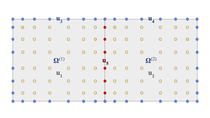
To mitigate the shortcomings of a global spectral method in solving an elliptic PDE such as in (1), we will partition into two rectangular non-overlapping subdomains and (we will alternatively call these subdomains “leaves” or “boxes”). We will discretize each subdomain using Chebyshev nodes, as we did for in Section 2.1. This leads to a total of points, since there is one shared face of points between and . A diagram of this discretization in 2D is presented in Figure 1, with denoting the shared face. We already know the data of the other faces ( in the figure) on both boxes as part of the Dirichlet boundary condition. If we can solve for the points on the shared face first, then we can solve for the interior of each subdomain separately using a spectral method as in Section 2.1, enforcing the PDE locally. To help solve for the shared face, we will add an additional condition to our problem: the Neumann derivative of on and must be equal on the shared face. In other words, we enforce continuity of the Neumann derivative.
To enforce this continuity, we need to find a numerical approximation to the Neumann derivative. This can be done using spectral differentiation matrices. In particular we form a Neumann operator matrix on each subdomain such that
Here are indices for each face of the subdomain boundary, with pointing in the direction, pointing in the direction, and pointing in the direction (respectively “left”, “right”, “down”, “up”, “back”, and “front” - in 2D and are omitted). obtains the Neumann derivative for each face, taking in both the boundary points and interior points as inputs. To obtain the Neumann derivatives using only , we combine with the solution operator to get
| (5) |
is the identity matrix and denotes the Dirichlet-to-Neumann (DtN) map for (also called the Poincaré-Steklov operator). For homogeneous PDEs we approximate the Neumann derivative entirely with , whereas the inhomogeneous case requires some contribution from the body load as seen in (2.2). Since maps from the box boundary to itself, it is a square matrix of size .
Borrowing terminology from Figure 1, let denote the various subsets of on discretized . Let denote the Neumann derivatives on the same points as , and let denote the DtNs on . Then, with a reindexing of some rows and columns of the DtNs,
| (6) |
By setting (Neumann derivative of the shared face) equal to itself, we get
| (7) |
Thus we can compute the shared face and , given by the Dirichlet boundary condition, and a new solution operator computed entirely from submatrices of the DtNs. This assumes a homogeneous PDE - if the problem is inhomogeneous, additional terms with the body load are present such as in (2.2). Once is solved, we can treat it as Dirichlet data for and , along with and , to get and .
This divide-and-conquer approach has a few advantages over a global spectral method. The solution operators and DtN maps for each subdomain can be computed separately, providing an easy source of parallelism. While the merged solution operator is still somewhat ill-conditioned, it is better conditioned than a global spectral matrix with the same domain size and degrees of freedom. In addition, nodes are more evenly spaced across the entire domain than in a global spectral method.
2.2.1 Merging with Corner and Edge Points
Since Chebyshev nodes include the ends of their interval, using them to discretize boxes produces nodes on the corners and edges. Corner nodes present a challenge in this method, since their Neumann derivative is ill-defined (in three dimensions this challenge extends to edge points as well, but for consistency we will also refer to these nodes as corner nodes). If our partial differential operator does not include mixed second order derivatives (such as in the Poisson equation or constant-coefficient Helmholtz), then the corner nodes do not impact the values of interior domain points through the solution operator due to the structure of spectral differentiation matrices, so we may simply drop them from our discretization: when merging boxes, we only consider the points on the interior of the shared face.
However, if does include mixed second order terms, then the corner points impact interior points through , so exclusion will significantly reduce accuracy. To make their role in the Neumann derivative unambiguous, we interpolate the box face points to Gaussian nodes (which do not include the ends of their interval) in this case. Then we define our DtN map , where is the Chebyshev-to-Gaussian interpolation operator, and is the Gaussian-to-Chebyshev interpolation operator. Once the shared face is solved, we then interpolate it back to Chebyshev nodes before applying the local solution operators. A projection operator is composed onto the Gaussian-to-Chebyshev interpolation matrix to preserve continuity at corner points.
We call the degree of the modified box exteriors . In the case of dropped corners . We can choose when we use Gaussian interpolation, but or is generally most effective. This means in practice the DtN maps are size .
2.3 Analogy to Sparse Factorization
One interpretation of this merge operation is as an analogy to factorization [21]. Consider Figure 1, simplifying it by considering the domain Dirichlet boundary terms parts of and respectively. Then we can represent our numerical partial differential operator (PDO) with
| (8) |
Here is the solution and is the body load on the interior of , split into the two subdomains and shared boundary. Because an elliptic PDO is a local operator there is no interaction through on by or by , so in those submatrices. However, both and , are local to the shared boundary where lies, so they both interact with the body load there, , through . To interpret the first two block rows, note that
| (9) |
This is similar to our solution operator formulation shown in (2.1), with the part of the subdomain boundary on now folded into . Next, let and . If we supply these vectors in place of in (8) and set , then the equation still holds with the same body loads and . Thus and are the particular solutions to our PDE on the interiors of , and with . Now consider an upper triangular matrix that satisfies
| (10) |
This linear system can be confirmed with (9). decouples our solutions into the particular solutions which are derived from our global Dirichlet BC without the subdomain-only (shared face) Dirichlet BC, and which is that subdomain-only boundary condition. Thus collects both components of our solutions - in effect it represents the end of solving the merged system, where we use and to get , and and to get . Next, let be a lower triangular matrix defined such that
| (11) |
To interpret this, note that
| (12) |
This has some resemblance to (7) when noting that encodes the impact of Dirichlet data without (and likewise is without ). If an additional operator was composed onto that resembled a Neumann derivative approximation following an inverse of the PDO, then it would closely resemble from (7). Another way to view (12) is that it breaks loads from decoupled on the two subdomains from , leaving another decoupled term in . By giving us from , can enable us to formulate a reduced problem that will solve for given - it performs the first part of the merge operation. To define this reduced problem, consider a block diagonal matrix where
| (13) |
This now represents a fully decoupled system for the particular solutions and shared boundary . However, we need to find a submatrix that satisfies this system. Such a can be found as
| (14) |
This formulation for includes the effect of on its body load () as well as terms that resemble the solution operators in (2.1) acting on only (). If we combine it with (12) then we see
| (15) |
This more closely resembles (7). Lastly, by combining the matrices together,
| (16) |
Thus is an LDU factorization of , with resembling the merge operations we derive via DtN maps, and resembling the interior solve for once we obtain the shared boundary data. This conceptualization will prove useful in justifying our algorithm for HPS.
3 Algorithm Description
In the previous section we discussed how to merge two subdomains of a boundary value problem together using DtN maps before solving each subdomain with a localized spectral method. Here we will briefly explain how the original Hierarchical Poincaré-Steklov method extends this concept to subdomains, before introducing the contributions of this work.
3.1 Hierarchical Poincare-Steklov: Traditional Solver
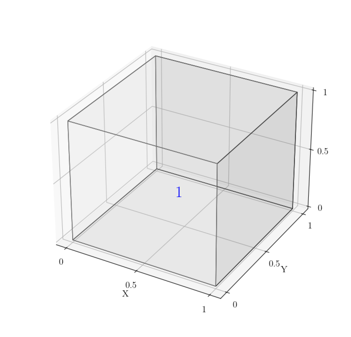
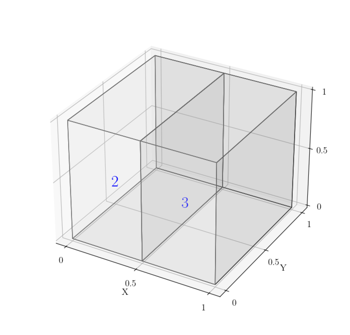
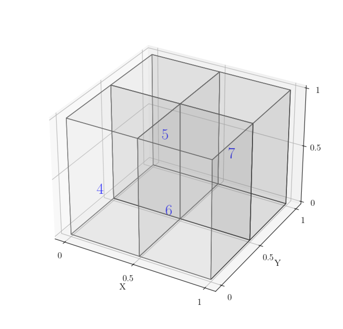
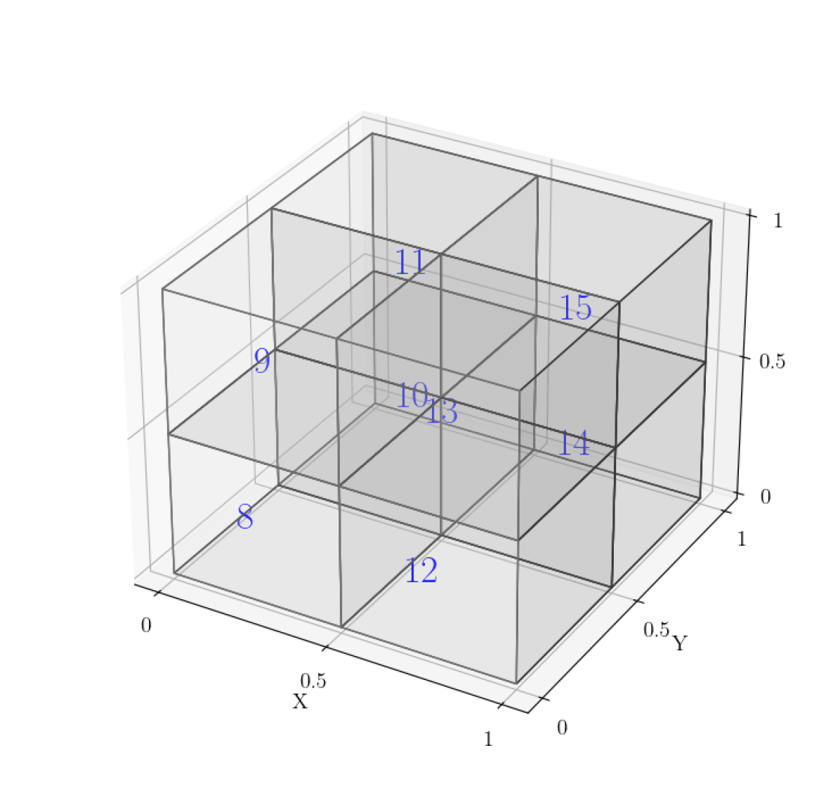
Given an elliptic PDE such as in (1) with a rectangular domain , we can hierarchically partition into a series of rectangular “box” subdomains, illustrated in Figure 2. Note that the boxes in each level are children of boxes in the previous level, with each box in level having 2 children in level , until we reach the final level of “leaf” boxes.
The HPS algorithm is split into two stages: the “build” stage, and the “solve” stage. In the build stage, we first construct solution and DtN maps for every leaf box in the final level of our discretization ( in Fig. 2). We then proceed in an upward pass, constructing solution maps for each box in the next level up using the leaf DtNs, following (7). These solution maps solve for the boundaries between paired leaf boxes (boxes 8 and 9, 10 and 11, 12 and 13, and 14 and 15 in Fig. 2). We then recursively construct solution and DtN maps for each level of the discretization, until we get a solution operator for which solves for one large face in the middle of the domain (between boxes 2 and 3 in Fig. 2). Once all solution operators are constructed, we proceed with the solve stage that follows a downward pass: using the Dirichlet boundary condition and the solution operator to solve for the middle boundary, then proceeding down and using each level’s solution operators to solve for subsequent box faces, until every leaf box has all faces solved. Then we solve for the leaf interiors using their local solution operators.
The method’s upward and downward passes recursively extend the formulation and use of solution operators we derived in Section 2.2. Similarly, they also resemble the LDU factorization described in Section 2.3. We can imagine the upward pass as similar to described there, with both encoding merge operations that reduce the body loads of the problem onto shared boundaries. then resembles formulating the final components of the merged solution operators and solving for the shared face points - it combines elements of the upward and downward pass. Lastly, is the end of the downward pass, obtaining the total solution. Given the similarities, it is not surprising that the classical algorithm for obtaining the DtN and solution operators of traditional HPS resembles multifrontal methods for sparse LU factorization [22, 23].
The original HPS method has a few significant drawbacks. The solution and DtN maps can be formed in parallel within each level, and prior work has used shared-memory models or MPI to accelerate this component [24, 25]. However, across levels these operators must be constructed recursively. This forces a large serial component to the algorithm. In addition, the method on a discretization with levels requires the storage of dense solution operators, which can be large especially for 3D problems. One can choose to recompute certain levels during the downward pass to reduce storage cost, but this greatly increases the computation time as a trade-off. In addition, higher level DtN maps tend to get increasingly ill-conditioned in this method, which can cause numerical challenges in the method’s stability (formulations using other merge operators such as impedance maps may be better conditioned [26]). Since each solution operator is applied separately in the downward pass, techniques such as pivoting are limited to improving the conditioning of one solution operator at a time - this is one way HPS differs significantly from sparse LU algorithms, despite the other similarities. Our contributions mitigate these problems with the original HPS method.
3.2 Two-Level HPS
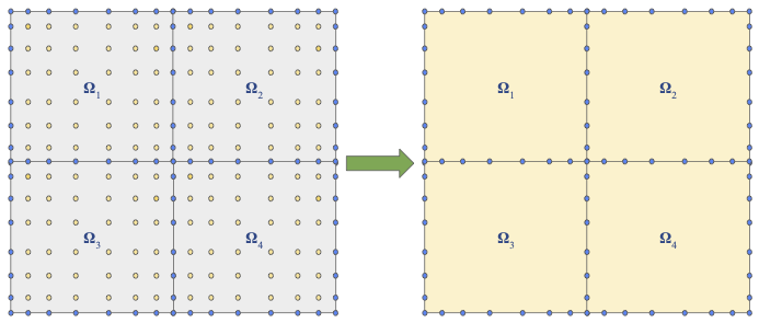
In this section we will discuss the contribution of our work: designing a direct solver for elliptic PDEs in 2D or 3D that utilizes the HPS method in a 2 level framework. Instead of constructing higher level solution and DtN operators, we use the leaf DtN maps to formulate a system that solves for all leaf boundaries concurrently. We use this system to acquire the leaf boundaries, then apply the leaf solution operators in parallel to solve for leaf interiors. With this approach we use the discretization for HPS to reduce the problem in a way analogous to static condensation, visualized in Figure 3. Similar to traditional HPS, our method can naturally be divided into a build stage and a solve stage.
3.2.1 Build Stage
As in previous sections suppose we have an elliptic PDE with a Dirichlet boundary condition on rectangular domain , in this case partitioned into a number of non-overlapping rectangular subdomains , each discretized with Chebyshev nodes. An example with 8 such boxes can be seen in Figure 4, similar to level in Figure 2. We know the value of numerical solution at every node on due to the Dirichlet boundary condition - we call this Dirichlet data . However, there are a number of box faces that do not lie on (see Figure 5(a), where there are 12 such faces). These must be solved before applying the leaf solution operators on each box to obtain on box interiors.
To solve for the shared faces we enforce continuity of the Neumann derivative using Dirichlet-to-Neumann maps as described in Section 2.2. However, each shared face depends on other shared faces since DtN maps require the entire box boundary data as input (unlike traditional HPS, where some box faces are solved earlier by different-level solution operators). So we must encode all shared faces in one coupled system. We construct this system using DtN maps and the relation between two boxes that share a boundary. Recall that each is size , where is either the size of a box face with corner points dropped, or the number of Gaussian nodes to which we interpolate (see Section 2.2.1). Thus the contribution of one box face to another face’s Neumann derivative via DtN is a submatrix of of size . We index our discretization points by box face so we can represent as a block matrix consisting of these submatrices. Referring back to (7) and Figure 1 in Section 2.2, each block row of (encoding the shared face between leaf boxes and ) looks like
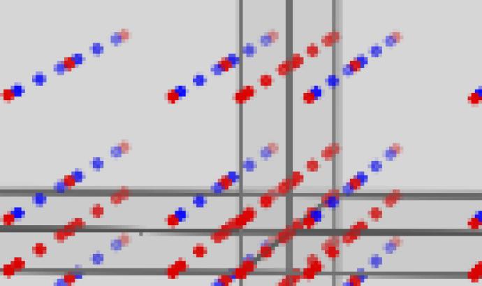
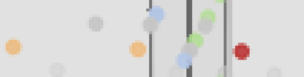
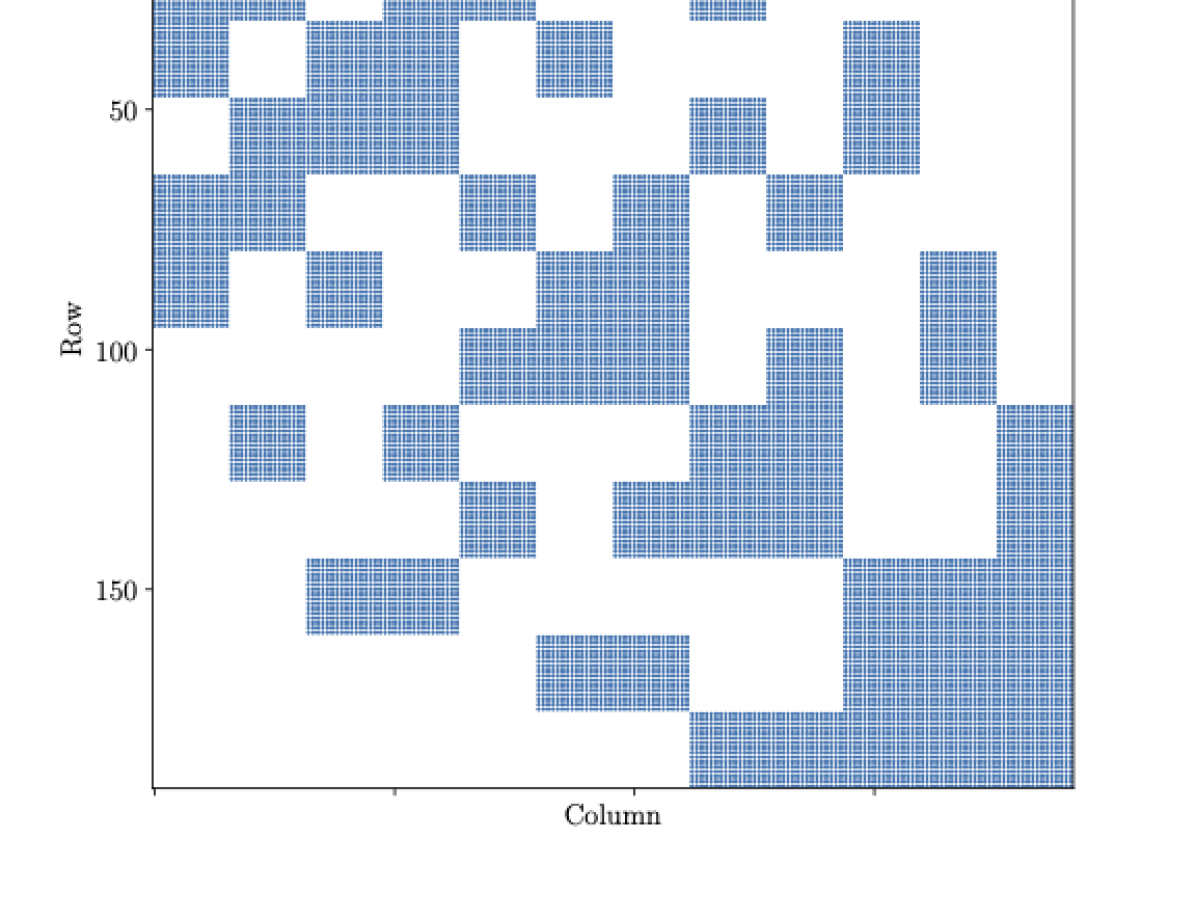
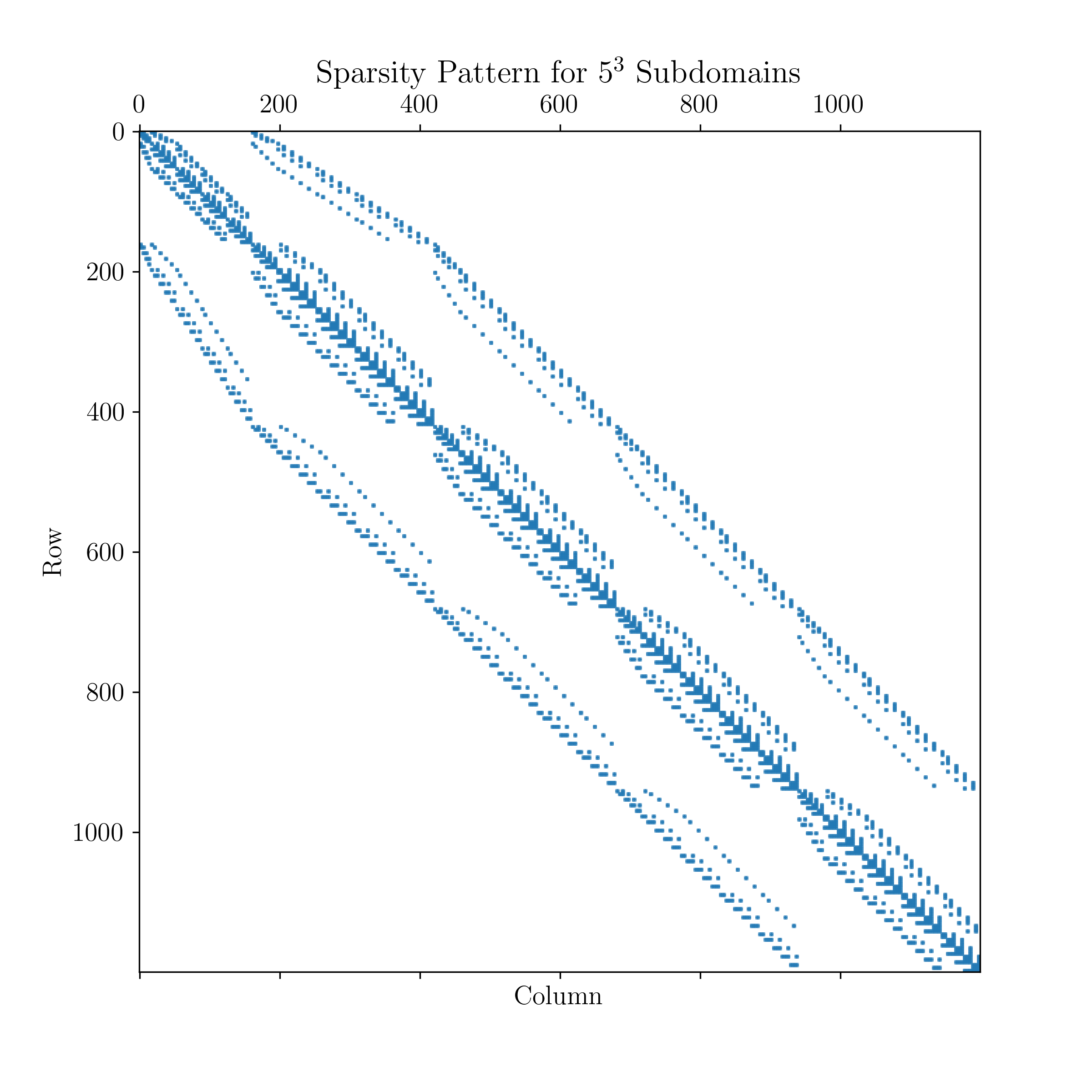
Recall is on the shared face between and , is on the other faces of , and is on the other faces of . Thus the block main diagonal is of size , and the block off-diagonals from and are each of size . This means each block row of has at most nonzero entries arranged into sized blocks (for some rows it is less, since portions of can lie on and be encoded in instead), so it has a distinctive block-sparse structure. This sparse structure can be seen for a problem with subdomains in Figure 5(b), and for a larger problem with subdomains in Figure 6. Note that the sparsity pattern is unaffected by the total number of subdomains.
Once is obtained, we may factorize it using a multilevel sparse solver such as MUMPS [27, 28]. An outline of the construction and factorization of is shown in Algorithm 1. First we construct the DtN maps , potentially with GPUs. Then we use submatrices of these DtN maps to formulate , which we then factorize.
3.2.2 Solve Stage
Once the factorized sparse system is obtained, we may use it as a direct solver for multiple variations in Dirichlet data and body load in the same boundary value problem. This is because the DtN maps and thus are only dependent on the problem’s partial differential operator. We find on the shared faces of our discretization by solving the sparse system,
| (18) |
Here is a right-hand-side specified by the Dirichlet data and body load. To solve for the box interior points (blue in Figure 4), we use the solution operators shown in (2.1). These operators enforce the PDE on the box interiors given the now-complete box boundary data. Each matrix is dense, but they can be formed and applied to box boundary data indepedently. Thus they are well-suited to use with batched linear algebra routines on GPUs, such as those offered in PyTorch [29] (the solution operators are also necessary to construct the DtN operators , but in practice it is often preferred to re-compute them and avoid transferring memory between CPU and GPU). The solve stage is detailed in Algorithm 2.
3.2.3 Advantages of the 2-Level Framework
In our solver we still discretize into a series of non-overlapping subdomains, but instead of constructing a hierarchical series of solution operators in an upward pass, we only form solution operators at the leaf level and use leaf DtN maps to form a larger system that solves for all of the subdomain boundaries concurrently - unlike the original methodology for HPS, which encodes different subdomain boundaries at each level. This resulting system is sparse, so we can factorize it using efficient sparse direct solvers such as those within the PETSc library [30].
Highly-optimized multifrontal solvers such as MUMPS can use various pivoting techniques such as partial threshold pivoting, relaxed pivoting [31], and tournament pivoting [32] to maximize numerical stability of a matrix factorization like sparse LU [33]. This enables accurate direct solves with potentially ill-conditioned systems. In theory such pivoting techniques could be used on the higher-level solution operators in traditional HPS to improve their stability (although these operators are dense, so sparse solvers could not be used). However, encoding solutions for all shared faces into one sparse matrix operator allows such pivoting techniques to be applied holistically on a much larger portion of the problem at once. This means the best possible pivoting can be applied, maximizing the factorization’s stability while preserving an optimal sparsity pattern. In effect we outsource the multilevel component of HPS to an optimized solver better equipped to handle its conditioning. Previous work has found other effective means to represent the HPS discretization as one large system, but required iterative techniques to solve [34]. Our approach preserves the original strength of HPS being a direct method.
In addition, the non-hierarchical nature of the formulation of - relying only on leaf DtN maps and not higher level DtN or solution operators - increases the method’s uniformity and parallelism. All DtN maps can be constructed in parallel; they are dense matrices, but that makes them well-suited to formulation on GPUs if available via batched linear algebra routines [35]. Similarly, the computation of the leaf solution operators in the solve stage may also be done in batch with GPUs. This allows us to use modern hardware to greatly improve the computational performance of the HPS method.
3.3 Asymptotic Cost
The build stage has an asymptotic cost of
We formulate the DtNs with embarrassingly parallel dense matrix operations that are well-suited for GPUs using batched linear algebra routines. As increases, its effect on the DtN size and run time is substantial - this is because of the need to invert a large block of the spectral differentiation submatrix , as shown in Algorithm 3. Nevertheless, we can still easily formulate DtNs in batch for . Even for larger where batched operations are impractical, formulating the DtNs in serial is relatively fast as shown in our numerical results. In practice the steepest cost in the build stage comes from the factorization of the sparse system, which for a 3D problem using a multilevel solver is . However, the sparse factorization is unaffected by the choice of and this cost is only required once per differential operator and domain discretization. Since the sparse system is relatively small (it has total entries with nonzero entries per row), it can be stored in memory and reused for multiple solves. For the solve stage, our asymptotic cost is
If we store the solution operators in memory then the interior box solves are only , but in practice it is typically preferred to reformulate the solution operators and avoid having to store and potentially transfer additional memory.
4 Numerical Experiments
4.1 Accuracy results - Poisson and Helmholtz Equations
We investigate the accuracy of our HPS solver on the homogeneous Poisson equation,
| (19) |
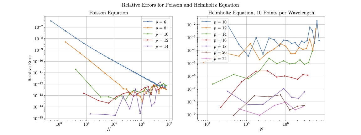
Here the Dirichlet boundary condition is defined so that it has a solution in its Green’s function. We compute numerical solutions to this equation across a range of block sizes and polynomial orders , comparing their relative -norm error to the Green’s function. The accuracy results are in Figure 7. We notice convergence rates of for and for until the relative error reaches , at which point it flattens (for larger the error reaches before a convergence rate can be fairly estimated). Subsequent refinement does not generally improve accuracy, but it does not lead to an increase in error either. This is likely due to the HPS discretization being fairly well-conditioned, especially compared to global spectral methods.
To assess our method’s accuracy on oscillatory problems we also evaluate it on the homogeneous Helmholtz equation with its Green’s function used as a manufactured solution with wavenumber ,
| (20) |
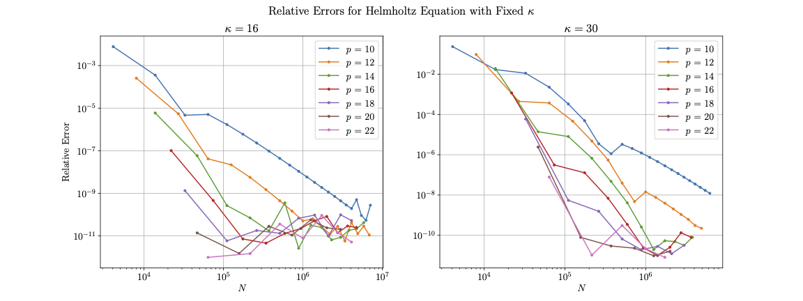
In Figure (8) we show relative -norm errors for our solver on Equation (20) with fixed wavenumbers and , which correspond to roughly 2.5 and 4.5 wavelengths on the domain, respectively. We see comparable convergence results to the Poisson equation, though the lower bound on relative error is somewhat higher for each problem ( for and for ). However, increasing the resolution further does not cause the error to diverge. Along with the results for Equation (19), this suggests our method remains stable when problems are over-resolved. Figure 7 shows the relative error for the Helmholtz equation with a varying , set to provide discretization points per wavelength. We see higher corresponds to a better numerical accuracy, while increasing does not improve results (since the wavenumber is also increased), but errors remain relatively stable. Since our method maintains accuracy while increasing degrees of freedom linearly with , it appears to not suffer from the pollution effect.
We then consider the gravity Helmholtz equation,
| (21) |
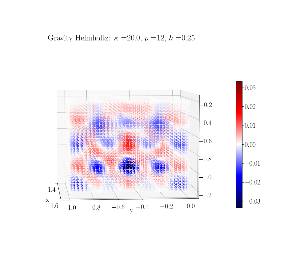
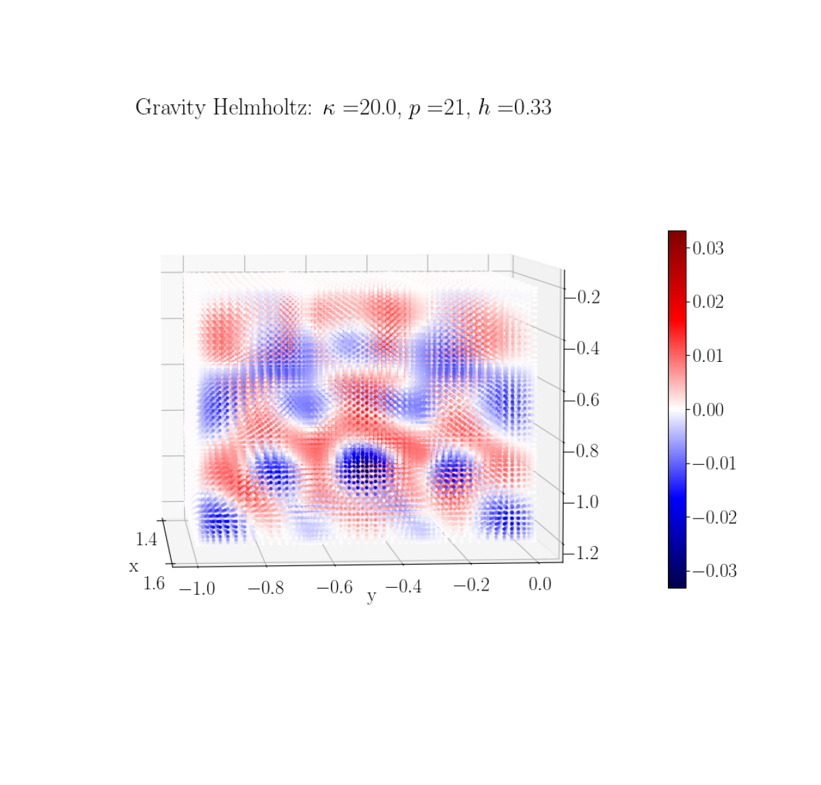
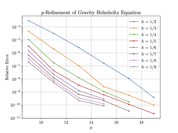
This equation adds a spatially-varying component to the wavenumber variation based on analogous to the effect of a gravitational field, hence the name [36]. Since , the variation is greater through than in the constant Helmholtz equation with the same . Unlike the previous Poisson and Helmholtz equations, equation (21) does not have a manufactured solution. It also produces relatively sharp gradients near the domain boundaries since there is a zero Dirichlet boundary condition, and it has a variable coefficient in spatial coordinates (specifically ). We investigate our solver’s accuracy by computing the relative -norm errors of our results to an over-resolved solution at select points. Figure 9 shows the solution of this problem using select and values, while Figure 10 shows these errors in the case of -refinement, for a range of values of . We can see our solver shows convergence for each .
4.2 Speed and scaling
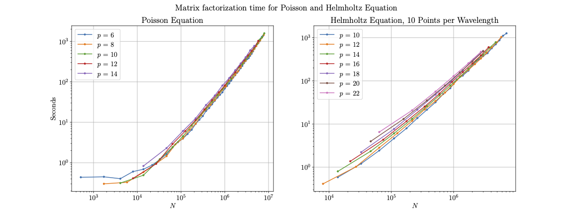
To evaluate the computational complexity of our HPS solver, we measure the execution times of its three components: the construction of the DtN operators used for the build stage, the factorization time for our sparse matrix constructed by the DtNs, and the solve time. We know the asymptotic cost of constructing the DtN operators is as shown in Equation (3.3). Figure (11) illustrates the run times for the build stage in solving the Poisson and Helmholtz equations detailed in Section 4.1, using batched linear algebra routines on an Nvidia V100 GPU. As expected, we observe a linear increase in runtime with -refinement (i.e. a higher with fixed ). The constant for the linear scaling in , though, increases sharply with higher values of .
A challenge with utilizing GPUs for DtN formulation is memory storage. In 3D each DtN map is size . Computing them requires the inversion of the spectral differentiation operator on interior points which is size . These matrices grow quickly as increases (at they are million and million entries, respectively). For larger problem sizes it is impossible to store all DtN maps on a GPU concurrently. Interior differentiation submatrices do not have to be stored beyond formulating their box’s DtN map, but they are much larger for high and present considerable overhead. To handle this memory concern we have implemented an aggressive two-level scheduler that stores a limited number of DtNs on the GPU at once, and formulates a smaller number of DtNs in batch at a time. For on a V100 GPU the best results occur when only one DtN is formulated at a time. However, we may still store multiple DtNs on the GPU before transferring them collectively to the CPU.
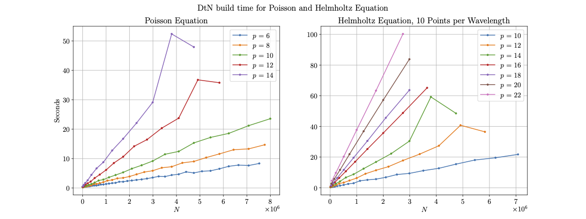
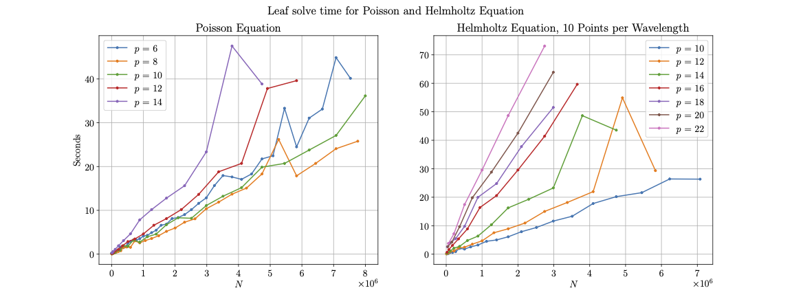
In Figure (12) we see the time to factorize the resulting sparse matrix for the build stage, using MUMPS. The expected asymptotic cost is . However, our results more closely resemble a lower cost of for up to 8 million. Overall the factorization time dominates the build stage of our method given its more costly scaling in and the reliance on CPUs through MUMPS. Lastly in Figure (13) we see the runtime for the leaf interior solves. These follow a linear scaling similar to the batched DtN construction.
4.3 Curved and non-rectangular domains
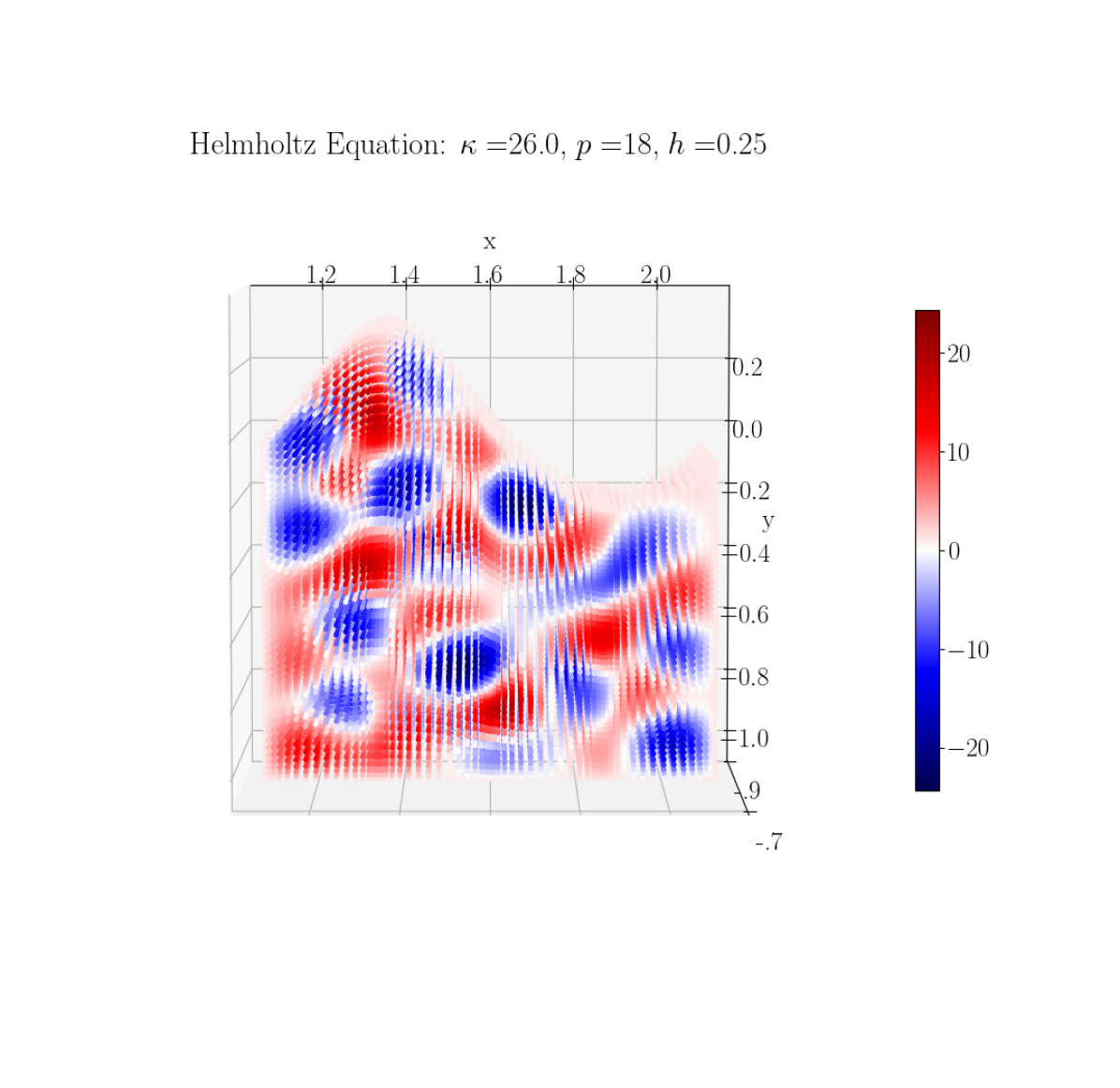
The HPS method has been extended to other problems such as surface PDEs [37], inverse scattering problems [38], and more generally non-rectangular domains. We can apply our HPS solver to non-rectangular domain geometries through the use of an analytic parameterization between the domain we wish to model, such as a sinusoidal curve along the -axis shown in Figure (14(a)), and a rectangular reference domain. These parameter maps extend the versatility of the solver, but feature multiple challenges in the implementation: they require variable coefficients for our differential operators; they may use mixed second order differential terms, i.e. where ; and (depending on the domain) may have areas that are near-singular, such as around the sharp point in Figure (14(a)). We investigate the accuracy of our solver on this sinusoidal domain for the Helmholtz equation as shown in Eq. (20), but now on the domain
| (22) |
We map (20) on to a cubic reference domain using the parameter map
| (23) |
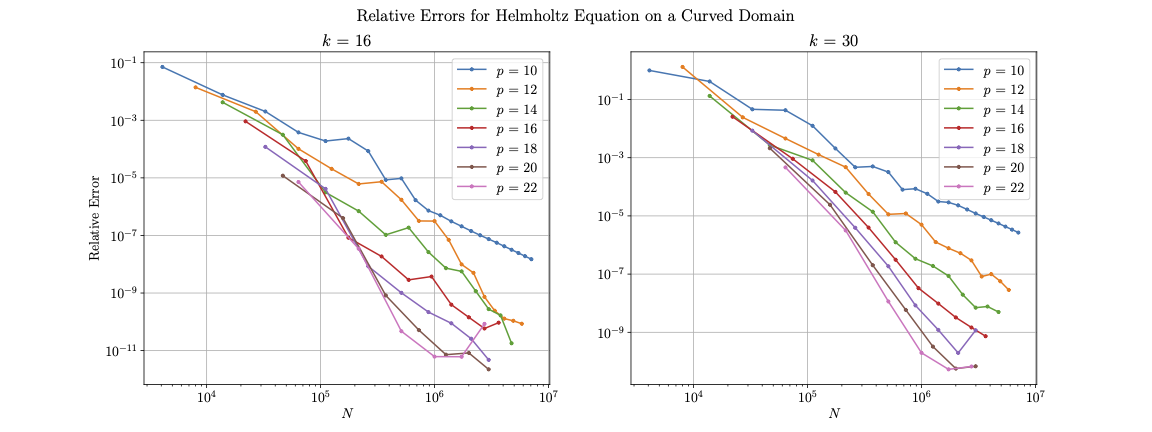
We test this problem with a manufactured solution in the Green’s function of the Helmholtz equation, with corresponding Dirichlet data matching our test in Section 4.1. A plot of this problem and the computed solution for wavenumber is shown in Figure 14(a), while convergence studies for this problem with and are shown in Figure 15. We observe a similar convergence pattern to the Helmholtz test on a cubic domain, although the speed of convergence is somewhat slower.
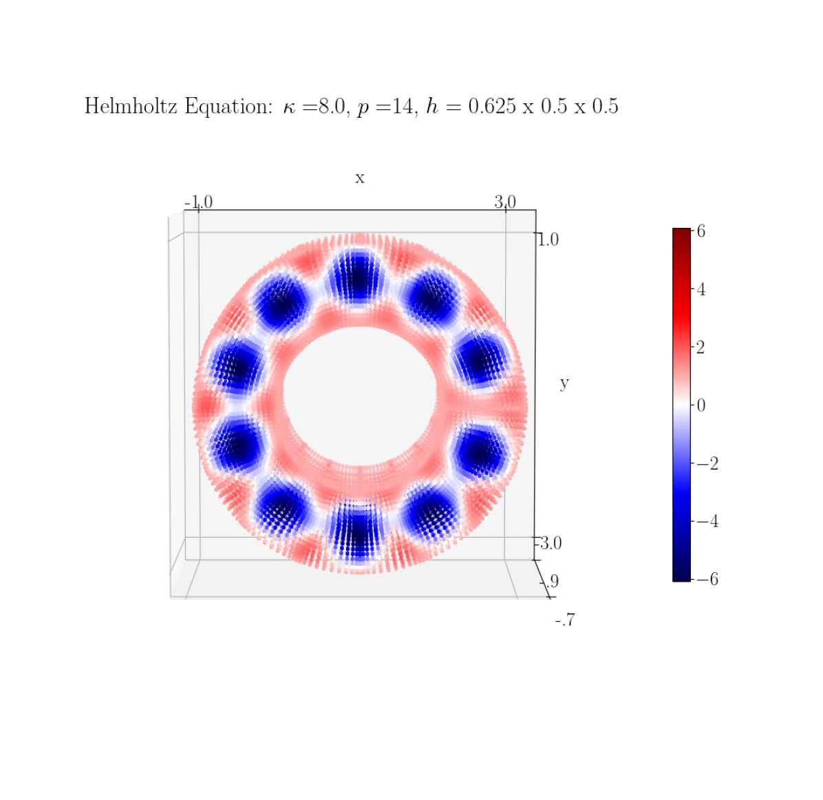
We also investigate our solver’s accuracy on the Helmholtz equation when the domain is a three-dimensional annulus, shown in Figure 14(b). We use an analytic parametrization to map this problem to a rectangular reference domain with higher resolution in the -axis and a periodic boundary condition. Relative errors in and are comparable to those for the problem on a curved domain.
5 Conclusion and Future Work
We have designed and implemented a two-level framework for the Hierarchical Poincaré-Steklov method that effectively decouples the hierarchical and dense portions of the method, using state-of-the-art multifrontal solvers to improve the stability of the first component, and GPUs to improve performance of the second component. Our code works for three-dimensional problems. However, there are still several directions for future work.
Although multifrontal solvers like MUMPS provide excellent stability, their use is also the main performance bottleneck in our implementation. GPU-based sparse solvers such as those in the NVIDIA cuDSS library may offer better performance. Alternatively, the reduced problem given to the sparse solver may itself be compressed into a two-level framework using SlabLU [39]. There are also potential performance gains by exploiting rank structure in the leaf operators, especially in the 3D discretization where these operators can be fairly large.
This implementation of HPS may be extended to other formulations of the method such as those using impedance maps rather than DtN maps, which may further improve conditioning. It may also be extended to adaptive discretizations [40, 41]. In addition to handling corner nodes, interpolation is also useful for implementing merge operators across subdomains with variable . Our method could also work in this adaptive case, although variable would somewhat alter the block-sparse structure of .
References
- [1] I. Babuška, F. Ihlenburg, E. T. Paik, S. A. Sauter, A generalized finite element method for solving the helmholtz equation in two dimensions with minimal pollution, Computer methods in applied mechanics and engineering 128 (3-4) (1995) 325–359.
- [2] I. M. Babuska, S. A. Sauter, Is the pollution effect of the fem avoidable for the helmholtz equation considering high wave numbers?, SIAM Journal on numerical analysis 34 (6) (1997) 2392–2423.
- [3] J. Galkowski, E. A. Spence, Does the helmholtz boundary element method suffer from the pollution effect?, Siam Review 65 (3) (2023) 806–828.
- [4] A. Townsend, S. Olver, The automatic solution of partial differential equations using a global spectral method, Journal of Computational Physics 299 (2015) 106–123.
- [5] J. P. Boyd, Chebyshev and Fourier spectral methods, Courier Corporation, 2001.
- [6] S. Olver, A. Townsend, A fast and well-conditioned spectral method, siam REVIEW 55 (3) (2013) 462–489.
- [7] T. Babb, A. Gillman, S. Hao, P.-G. Martinsson, An accelerated poisson solver based on multidomain spectral discretization, BIT Numerical Mathematics 58 (2018) 851–879.
- [8] A. Gillman, P.-G. Martinsson, A direct solver with o(n) complexity for variable coefficient elliptic pdes discretized via a high-order composite spectral collocation method, SIAM Journal on Scientific Computing 36 (4) (2014) A2023–A2046.
- [9] A. T. Patera, A spectral element method for fluid dynamics: laminar flow in a channel expansion, Journal of computational Physics 54 (3) (1984) 468–488.
- [10] Y. Maday, R. Munoz, Spectral element multigrid. ii. theoretical justification, Journal of scientific computing 3 (1988) 323–353.
- [11] A. Yeiser, A. A. Townsend, A spectral element method for meshes with skinny elements, arXiv preprint arXiv:1803.10353 (2018).
- [12] P. Martinsson, The hierarchical poincaré-steklov (hps) solver for elliptic pdes: A tutorial, arXiv preprint arXiv:1506.01308 (2015).
- [13] P.-G. Martinsson, Fast direct solvers for elliptic PDEs, SIAM, 2019.
- [14] T. Babb, P.-G. Martinsson, D. Appelö, Hps accelerated spectral solvers for time dependent problems: Part i, algorithms, in: Spectral and High Order Methods for Partial Differential Equations ICOSAHOM 2018: Selected Papers from the ICOSAHOM Conference, London, UK, July 9-13, 2018, Springer International Publishing, 2020, pp. 131–141.
- [15] K. Chen, D. Appelö, T. Babb, P.-G. Martinsson, Fast and high-order approximation of parabolic equations using hierarchical direct solvers and implicit runge-kutta methods, Communications on Applied Mathematics and Computation (2024) 1–21.
- [16] S. Hao, P.-G. Martinsson, A direct solver for elliptic pdes in three dimensions based on hierarchical merging of poincaré–steklov operators, Journal of Computational and Applied Mathematics 308 (2016) 419–434.
- [17] A. Yesypenko, P.-G. Martinsson, GPU optimizations for the hierarchical poincaré-steklov scheme, in: International Conference on Domain Decomposition Methods, Springer, 2022, pp. 519–528.
- [18] D. Fortunato, N. Hale, A. Townsend, The ultraspherical spectral element method, Journal of Computational Physics 436 (2021) 110087.
- [19] L. N. Trefethen, Finite difference and spectral methods for ordinary and partial differential equations, Cornell University-Department of Computer Science and Center for Applied …, 1996, Ch. 8.
- [20] A. Gillman, P.-G. Martinsson, An o (n) algorithm for constructing the solution operator to 2d elliptic boundary value problems in the absence of body loads, Advances in Computational Mathematics 40 (2014) 773–796.
- [21] T. A. Davis, Direct methods for sparse linear systems, SIAM, 2006.
- [22] A. George, Nested dissection of a regular finite element mesh, SIAM journal on numerical analysis 10 (2) (1973) 345–363.
- [23] P. R. Amestoy, T. A. Davis, I. S. Duff, An approximate minimum degree ordering algorithm, SIAM Journal on Matrix Analysis and Applications 17 (4) (1996) 886–905.
- [24] N. N. Beams, A. Gillman, R. J. Hewett, A parallel shared-memory implementation of a high-order accurate solution technique for variable coefficient helmholtz problems, Computers & Mathematics with Applications 79 (4) (2020) 996–1011.
- [25] D. Chipman, Ellipticforest: A direct solver library for elliptic partial differential equations on adaptive meshes, Journal of Open Source Software 9 (96) (2024) 6339.
- [26] A. Gillman, A. H. Barnett, P.-G. Martinsson, A spectrally accurate direct solution technique for frequency-domain scattering problems with variable media, BIT Numerical Mathematics 55 (2015) 141–170.
- [27] P. R. Amestoy, I. S. Duff, J.-Y. L’Excellent, J. Koster, Mumps: a general purpose distributed memory sparse solver, in: International Workshop on Applied Parallel Computing, Springer, 2000, pp. 121–130.
- [28] J. Pan, L. Xiao, M. Tian, T. Liu, L. Wang, Heterogeneous multi-core optimization of mumps solver and its application, in: Proceedings of the 2021 ACM International Conference on Intelligent Computing and Its Emerging Applications, 2021, pp. 122–127.
- [29] S. Imambi, K. B. Prakash, G. Kanagachidambaresan, Pytorch, Programming with TensorFlow: solution for edge computing applications (2021) 87–104.
- [30] S. Balay, S. Abhyankar, M. Adams, J. Brown, P. Brune, K. Buschelman, E. Constantinescu, A. Dener, J. Faibussowitsch, W. Gropp, et al., Petsc/tao users manual revision 3.22, Tech. rep., Argonne National Laboratory (ANL), Argonne, IL (United States) (2024).
- [31] I. S. Duff, S. Pralet, Towards stable mixed pivoting strategies for the sequential and parallel solution of sparse symmetric indefinite systems, SIAM Journal on Matrix Analysis and Applications 29 (3) (2007) 1007–1024.
- [32] L. Grigori, J. W. Demmel, H. Xiang, Communication avoiding gaussian elimination, in: SC’08: Proceedings of the 2008 ACM/IEEE Conference on Supercomputing, IEEE, 2008, pp. 1–12.
- [33] P. Amestoy, J.-Y. L’Excellent, T. Mary, C. Puglisi, Mumps: Multifrontal massively parallel solver for the direct solution of sparse linear equations, in: EMS/ECMI Lanczos prize, ECM conference, Sevilla, 2024.
- [34] J. P. Lucero Lorca, N. Beams, D. Beecroft, A. Gillman, An iterative solver for the hps discretization applied to three dimensional helmholtz problems, SIAM Journal on Scientific Computing 46 (1) (2024) A80–A104.
- [35] J. Dongarra, S. Hammarling, N. J. Higham, S. D. Relton, M. Zounon, Optimized batched linear algebra for modern architectures, in: European Conference on Parallel Processing, Springer, 2017, pp. 511–522.
- [36] A. H. Barnett, B. J. Nelson, J. M. Mahoney, High-order boundary integral equation solution of high frequency wave scattering from obstacles in an unbounded linearly stratified medium, Journal of Computational Physics 297 (2015) 407–426.
- [37] D. Fortunato, A high-order fast direct solver for surface pdes, SIAM Journal on Scientific Computing 46 (4) (2024) A2582–A2606.
- [38] C. Borges, A. Gillman, L. Greengard, High resolution inverse scattering in two dimensions using recursive linearization, SIAM Journal on Imaging Sciences 10 (2) (2017) 641–664.
- [39] A. Yesypenko, P.-G. Martinsson, SlabLU: a two-level sparse direct solver for elliptic PDEs, Advances in Computational Mathematics 50 (4) (2024) 90.
- [40] P. Geldermans, A. Gillman, An adaptive high order direct solution technique for elliptic boundary value problems, SIAM Journal on Scientific Computing 41 (1) (2019) A292–A315.
- [41] D. Chipman, D. Calhoun, C. Burstedde, A fast direct solver for elliptic pdes on a hierarchy of adaptively refined quadtrees, arXiv preprint arXiv:2402.14936 (2024).