A Two-stage Approach for Variable Selection in Joint Modeling of Multiple Longitudinal Markers and Competing Risk Outcomes
Abstract
Background In clinical and epidemiological research, the integration of longitudinal measurements and time-to-event outcomes is vital for understanding relationships and improving risk prediction. However, as the number of longitudinal markers increases, joint model estimation becomes more complex, leading to long computation times and convergence issues. This study introduces a novel two-stage Bayesian approach for variable selection in joint models, illustrated through a practical application.
Methods Our approach conceptualizes the analysis in two stages. In the first stage, we estimate one-marker joint models for each longitudinal marker related to the event, allowing for bias reduction from informative dropouts through individual marker trajectory predictions. The second stage employs a proportional hazard model that incorporates expected current values of all markers as time-dependent covariates. We explore continuous and Dirac spike-and-slab priors for variable selection, utilizing Markov chain Monte Carlo (MCMC) techniques.
Results The proposed method addresses the challenges of parameter estimation and risk prediction with numerous longitudinal markers, demonstrating robust performance through simulation studies. We further validate our approach by predicting dementia risk using the Three-City (3C) dataset, a longitudinal cohort study from France.
Conclusions This two-stage Bayesian method offers an efficient process for variable selection in joint modeling, enhancing risk prediction capabilities in longitudinal studies. The accompanying R package VSJM, which is freely available at https://github.com/tbaghfalaki/VSJM, facilitates implementation, making this approach accessible for diverse clinical applications.
1 Introduction
In many clinical studies, longitudinal measurements are repeatedly collected for each subject at different time points until an event such as death or drop-out occurs. It is also common to have multiple longitudinal measurements in a study. For example, in the context of HIV/AIDS studies, two important markers that are often repeatedly measured until death or drop-out are HIV-RNA and CD4 [24]. In most of these types of studies, the number of longitudinal markers under investigation and the number of explanatory variables is large. Estimating the association between longitudinal markers and time-to-event outcomes, as well as determining the effect of explanatory variables on event risks, is crucial in modern medicine [26, 47, 29, 16, 61], in particular, for the development of individual risk prediction models [39, 40].
For this purpose, joint models for longitudinal and time-to-event outcomes
that combine mixed models and time-to-event models,
have received considerable attention over the past decades.
Interesting reviews on joint modeling can be found in [49, 35, 1] and [63].
From a computational point of view, the R software now offers some options: JMBayes [41], JMBayes2 [38], INLAjoint [44], and stan_jm modelling function in the rstanarm package [10]. The Bayesian implementation of joint models with multiple markers is available through INLAjoint [44] and JMBayes2 [38], but dealing with a large number of markers still poses computational difficulties due to the large number of random effects and parameters in these models.
For this purpose, [5] propose a novel two-stage joint modeling approach (TSJM). In the first stage, joint models are estimated for each marker and the time-to-event. In the second stage, the predicted values of linear predictor of each marker are used as time-dependent covariates in a semi-parametric Cox model. This method enhances tractability and reduces bias from informative dropouts.
When multiple longitudinal markers and large number of time-invariant explanatory variables, are considered, the selection of the most predictive variables is challenging. Traditionally this has been performed through model comparison criteria such as Akaike Information Criterion (AIC), Bayesian Information Criterion (BIC), or Deviance Information Criterion (DIC). The use of these criteria for complex models in the presence of a large number of candidate models is not feasible due to the computational complexity associated with evaluating these criteria for complex models with numerous parameters and candidate models. Consequently, traditional criteria may not effectively guide model selection in such complex scenarios. This has led to the exploration of alternative strategies, such as variable selection, to address these challenges and identify the most appropriate model.
It involves choosing appropriate variables from a complete list and removing those that are irrelevant or redundant. The purpose of such selection is to determine a set of variables that will provide the best fit for the model in order to make accurate predictions [15]. In general, variable selection in the frequentist paradigm involves the utilization of a penalized likelihood approach, which considers various forms of penalty functions. These include the least absolute shrinkage and selection operator (LASSO), the smoothly clipped absolute deviation (SCAD), and the adaptive least absolute shrinkage and selection operator (ALASSO) [11].
In the Bayesian framework, the selection of appropriate priors plays a pivotal role, similar to the regularization and shrinking techniques employed in frequentist variable selection methods. Properly chosen priors not only inform the prior beliefs about model parameters but also contribute to the regularization of the model, aiding in the prevention of overfitting and the promotion of model parsimony [21].
In this paper, we delve into the realm of Bayesian variable selection, where the careful selection of priors allows for the automatic identification of relevant predictors while appropriately handling model complexity [22]. Various types of priors have been proposed for variable selection, including spike-and-slab priors [32, 22, 34], horseshoe prior [12], and Laplace (i.e., double-exponential) prior [55].
Our investigation focuses on two prominent types of priors: continuous and Dirac spike priors. These priors strike a balance between flexibility and simplicity, offering practical advantages in the context of variable selection [46]. By exploring the implications and effectiveness of these priors, we aim to provide insights into their utility and contribute to the ongoing discourse surrounding Bayesian variable selection methodologies.
Variable selection methods in joint modeling have been explored across various studies, each offering unique insights into different aspects of the modeling process. [25] employed a penalized likelihood approach with adaptive LASSO penalty functions to select fixed and random effects in joint modeling of one longitudinal marker and time-to-event data. [60] extended this approach to the joint analysis of longitudinal data and interval-censored failure time data, utilizing penalized likelihood-based procedures to simultaneously select variables and estimate covariate effects. [23] adopted gradient boosting for variable selection in joint modeling, providing an alternative method for addressing this task.
[13] utilized L1 penalty functions to select random effects and off-diagonal elements in the covariance matrix in the survival sub-model. Their focus was on joint modeling of multiple longitudinal markers and time-to-event data within the frequentist paradigm. [53] considered simultaneous parameter estimation and variable selection in joint modeling of longitudinal and survival data using various penalized functions. [56] utilized a B-spline decomposition and penalized likelihood with adaptive group LASSO to select the relevant independent variables and distinguish between the time-varying and time-invariant effects for the two sub-models.
On the Bayesian side, [52] proposed a semiparametric joint model for analyzing multivariate longitudinal and survival data. They introduced a Bayesian Lasso method with independent Laplace priors for parameter estimation and variable selection. However, these studies primarily focused on scenarios with a limited number of longitudinal markers and did not address cases where the number of markers is high.
Additionally, dynamic prediction in the context of variable selection in joint modeling remains unexplored in the literature reviewed here.
In this paper, we consider variable selection, including the selection of both the longitudinal markers and the time-invariant covariates, in the joint modeling of multiple longitudinal measurements and competing risks outcomes. This is the first study to specifically address variable selection in this context.
For this purpose, we are faced with two issues. The first challenge is estimating joint models including a large number of longitudinal markers, which may be unfeasible. The second challenge, which involves variable selection, is addressed by using a spike-and-slab prior in a Bayesian paradigm.
As a summary, we propose a new two-stage approach for variable selection of multiple longitudinal markers and competing risks outcomes when the number of longitudinal markers and covariates is large, and the estimation of the full joint model including all the markers and covariates is intractable. Using a Bayesian approach, the first stage involves estimating one-marker joint models for the competing risks and each longitudinal marker as in [5]. This avoids the bias caused by informative dropout. In the second stage, extending TSJM, we estimate a cause-specific hazard model for the competing risks outcome using a Bayesian approach allowing variable selection using a Bayesian approach allowing variable selection. This model includes time-dependent covariates and incorporates spike-and-slab priors. The explanatory variables in the hazard model consist of the estimates of functions derived from the random effects and parameters obtained from the initial stage of jointly modeling each longitudinal marker.
We provide an R-package VSJM that implements the proposed methods which is available at https://github.com/tbaghfalaki/VSJM.
This paper is organized as follows: In Section 2, we describe our variable selection approach, which includes introducing longitudinal and competing risks sub-models, reviewing parameter estimation in MMJM, and finally describing our proposed two-stage approach for Bayesian variable selection. Section 3 focuses on dynamic prediction using the proposed approach. Section 4 presents a simulation study comparing the behavior of the variable selection two-stage approach with the oracle joint model in terms of variable selection and dynamic prediction.
In Section 5, the proposed approach is applied to variable selection and the risk prediction of dementia in the Three-City (3C) cohort study [2]. Finally, the last section of the paper includes a conclusion of the proposed approach.
2 Variable selection for Joint modeling
The observed time is where denotes the censoring time and the time to the event . Also, the event indicator is denoted as , where corresponds to censoring and to competing events. Denote the measure of the th longitudinal marker for the th subject at time by . As a result, consider a sample from the target population.
2.1 Longitudinal sub-model
A multivariate linear mixed-effects model is considered for the multiple longitudinal markers as follows:
| (1) |
where . We assume that
| (2) |
where and are the design vectors at time for the -dimensional fixed effects and -dimensional random effects , respectively. We assume that takes into account the association within and between the multiple longitudinal markers such that , and is a covariance matrix, where . It is assumed that is independent of , .
2.2 Competing risks sub-model
For each of the causes, a cause-specific proportional hazard model is postulated. The risk of an event is assumed to be a function of the subject-specific linear predictors and of time-invariant covariates as follows [40]:
| (3) |
where denotes the baseline hazard function for the th cause, is a vector of covariates with corresponding regression coefficients , and represents the vector of association parameters between the longitudinal markers and cause . There are different approaches for specifying the baseline hazard function in joint modeling [40]. The methodology is not restricted to a specific form of the baseline hazard, and we consider a piecewise constant baseline hazard [27]. Therefore, a finite partition of the time axis is constructed as , such that . Thus, there are intervals such as . We consider a constant baseline hazard for each interval as .
2.3 Parameter estimation of the multi-marker joint model
Let and represent the unknown parameters for the th longitudinal marker and the time to event outcomes, respectively, excluding the covariance matrix . Let . If , , and , the joint likelihood function for models (1) and (3) is as follows:
where represents the cumulative hazard function of Equation (3), and the densities of the univariate normal distribution with mean and variance , and the -variate normal distribution with mean and covariance matrix , are denoted as and , respectively.
In the frequentist paradigm, parameter estimation can be computed by maximizing (2.3), which involves the use of numerical integration [14, 48]. This integration will be more challenging when the number of outcomes increases. In the Bayesian paradigm [57, 42, 4, 30], the following joint posterior distribution can be used for parameter estimation:
where , and are the corresponding prior distributions for the unknown parameters. In this paper, we consider zero-mean normal distributions with a large variance as prior distributions for the regression coefficients and association parameters. A vague inverse gamma distribution is considered as the prior distribution for the variance of errors. An inverse Wishart distribution with degrees of freedom equal to the dimension of the random effects and an identity scale matrix is utilized as the prior for the variance of the random effects. The parameters of the baseline hazard are assumed to follow a gamma distribution with a mean of 1 and a large variance. In the next section, we introduce our proposed two-stage approach for variable selection of longitudinal markers and covariates in a Bayesian paradigm.
2.4 Two-stage joint modeling of multiple longitudinal measurements and competing risks
The proposed method adopts a two-stage approach for variable selection in joint modeling, targeting the selection of markers (or time-varying covariates) and time-invariant covariates. This approach is specifically designed for handling multiple longitudinal markers and time-to-event outcomes, with the primary goal of avoiding bias caused by informative dropouts.
This relies on the idea of TSJM approach of [5] but considering competing risks and replacing the estimation of a Cox model by partial likelihood in the second stage by a fully Bayesian approach allowing variable selection.
The first stage involves estimating one-marker joint models for the competing risks and each marker. In the second stage, we estimate cause-specific proportional hazard models including the time-invariant explanatory variables and the predicted current values of the linear predictor of each longitudinal markers obtained from stage 1. Therefore, the approach consists of two stages, outlined as follows:
- Stage 1
-
For each , , estimate the joint model for the longitudinal marker and competing risks. The one-marker JMs are estimated using the joint posterior distribution given by equation 2.3 for . Then, predict the random effects and the linear predictor , for marker using the empirical mean of the posterior distribution , where represents the estimated parameters for the one-marker joint model for the th longitudinal marker. This first stage allow the estimation of without the bias due to informative dropout but neglecting the correlation between the markers..
- Stage 2
-
In the second stage, the values of are included as time-varying covariates in a proportional hazard model to estimate parameters and , as well as the baseline hazard from (3). The cumulative hazard function of (3) can be approximated using Gaussian quadrature [9, 54]. In the Bayesian paradigm, the following joint posterior distribution is considered:
where , such that, denotes the vector of the piecewise constant baseline hazard for cause . The prior distributions for unknown parameters are the same as those considered for Equation 2.3.
2.5 Bayesian variable selection
As above, we consider the prior distributions , where is a large value, , and . Our purpose is to implement variable selection for the regression coefficients of the cause-specific hazard model (3) and the association parameters of (3). Therefore, we consider two different prior distributions, including continuous spike and Dirac spike, for them.
2.5.1 Continuous spike
The continuous spike [32, 22, CS,] prior for is given by
| (11) |
Also, the CS prior for the association parameter is given by
| (16) |
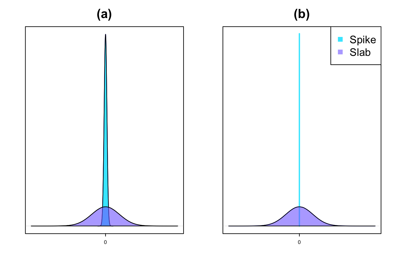
where, in (11) and in (16) are a small fixed value (e.g., or ) and represents a spike prior. The latent variable in (11) (or in (16)) is considered to account for the significance of the parameter. For example, if , then the distribution of will be , and can be considered as significant. This leads us to have a slab prior. A graphical example of CS prior can be found in panel (a) of Figure 1.
2.5.2 Dirac spike
We exploit a Dirac spike-and-slab prior [22, 34, DS,] similar to that proposed by [58]. For this purpose, the DS prior for is given by
| (20) |
where represents a point mass at . It is defined as when and when is non-zero, i.e., . Also, the DS prior for the association parameter is given by
| (24) |
A graphical example of the DS prior can be found in panel (b) of Figure 1. For implementing Bayesian inference, a block Gibbs sampler is used in conjunction with the Metropolis-Hastings algorithm. For this purpose, we require all of the full conditional distributions. The Markov Chain Monte Carlo (MCMC) sampling is performed using “JAGS” [37, 36] and the R2jags [51] package is utilized as an interface between R and JAGS. The package automatically computes the full conditional posterior distributions for all parameters and models. We refer to this approach as Variable Selection for Joint Modeling (VSJM). The methodology has been implemented in the R package VSJM.
2.6 Statistical inference
To select significant variables in the covariates of the cause-specific hazard model and by considering Equation (11) or (20), the following hypothesis tests are conducted:
| (27) |
Also, to select significant longitudinal markers based on the association parameters and by considering Equation (16) or (24), the following hypothesis tests are considered:
| (30) |
In practice, when implementing the hypotheses (27) and (30) for CS, it is possible to consider the following equivalent hypotheses, respectively:
| (33) |
| (36) |
We consider two different Bayesian testing approaches for evaluating these hypotheses: a local Bayesian false discovery rate [18] and a Bayes factor [28].
2.6.1 Continuous spike
Local Bayesian false discovery rate
Let denote the data in the study. The set of unknown parameters of the CS model is denoted as . Let represent the posterior probability of the null hypothesis. This is the probability of making a false discovery for a significant covariate, which is called the local Bayesian false discovery rate for
(denoted by ) by Efron [18]. The small values of indicate strong evidence for the presence of a significant covariate. For computing of Equation (33), we obtain
where is an indicator function and
denotes the , generated sample of
using the Gibbs sampler.
The lBFDR is a procedure for investigating the null hypothesis. It is an empirical Bayes version of the methodology proposed by [7]. This approach focuses on densities instead of tail areas [19, 20, 17]. Efron [17] demonstrated that the false discovery rate control rule proposed by [7] can be expressed in terms of empirical Bayes. They also showed that the desired control level (referred to as ) for Benjamini-Hochberg testing of single tests can be regarded as the desired control level for local Bayes false discovery rate (lBFDR) as well. Based on Remark B of [17], if the value of lBFDR is not greater than 0.05 (the desired control level), the null hypothesis will be rejected. In fact, the interpretation of the lBFDR value is analogous to the frequentist’s p-value. LBFDR values less than a specified level (e.g., 0.05) of significance provide stronger evidence against the null hypothesis [45, 59]. The value of 0.05 in the context of variable selection is also considered a threshold for lBFDR by [31] and [6].
Thus, a local Bayesian false discovery rate of 0.05 is considered in this paper.
Bayes factor
The Bayes factor for testing (33) is defined as
which describes the evidence of against . Note that as are assumed independent. Hence,
Also, since ,
| (37) |
Unlike , a large value of indicates strong evidence in favor of . Also, a widely cited table is provided by [28]. This table is based on and can be used to quantify the support that one model has over another.
All comments mentioned above can also be applied to the hypothesis testing of equations (36).
2.6.2 Dirac spike
The strategy for performing lBFDR and BF for DS is to define indicator variables as , and , such that
By considering these indicator variables, all of those described for the CS can also be used for the DS.
3 Dynamic predictions
3.1 Dynamic predictions from VSJM
The joint modeling of longitudinal measurements and time-to-event outcomes is a popular methodology for calculating dynamic prediction (DP). The DP represents the risk predictions for subject who has survived up to time point , taking into account longitudinal measurements and other information available until time . Consider the notation described in Section 2. Let the proposed joint models be fitted to a random sample, which is referred to as training data. For validation purposes, we are interested in predicting the risk of subjects in a new set of data called the validation set. The longitudinal measurements until time are denoted by and given by . Additionally, the vector of available explanatory variables until time is and given by . Let denote the event of interest, then, for the landmark time and the prediction window , the risk probability is as follows:
| (38) |
where is a vector of all unknown parameters of the model, including which is estimated at stage 1, and which is estimated at stage 2, and represents the true event time for the th subject. The predicted probability (38) can be computed as:
| (39) |
where represents the survival probability to survive to both events given random effects. The first order approximation for estimating this quantity [39, 5] is given as follows:
where are estimated based on the training data.
To predict , we consider the one-marker joint models for each marker and predict the -dimensional random effect given . This is denoted by , where represents the estimated parameters for the one-marker joint model in the first stage of VSJM. Merge the predicted random effects to obtain the -dimensional predicted random effect .
For Monte-Carlo approximation of (39), we follow the same strategy as those discussed in [62]. For this aim,
consider a realization of the generated MCMC sample for estimating the unknown parameters from the one-marker JM for marker in the training data, denoted .
Draw values from the posterior distribution . For
Calculate any desired quantity from the generated chains, such as percentiles, to determine the credible interval.
3.2 Reducing bias in dynamic predictions from VSJM
To reduce estimation biases resulting from variable selection, we propose incorporating an additional stage to calculate dynamic predictions. After variable selection using CS or DS prior, we recommend re-estimating the proportional hazard model by substituting CS or DS with non-informative normal priors for the association parameters of the selected markers and the regression coefficients of the selected covariates. Then calculate the DP as described in Section 3.1.
3.3 Measures of prediction accuracy
We use the Area Under the Receiver Operating Characteristics Curve (AUC) and the Brier Score (BS) to assess the predictive performance of prediction models [50]. AUC represents the probability that the model correctly ranks a randomly chosen individual with the disease higher than a randomly chosen individual without the disease based on their predicted risks Additionally, BS measures the preduction accuracy by quantifying the mean squared error of prediction. For censored and competing time-to-event and time-dependent markers, a non-parametric inverse probability of censoring weighted estimator of AUC and BS was proposed by [8] and utilized in this paper.
4 Simulation study
4.1 Design of simulation study
A simulation study was conducted to assess the effectiveness of the proposed VSJM approach for variable selection and risk prediction. To evaluate the effectiveness of the proposed approaches for variable selection, we examine three distinct criteria: the true positive rate (TPR), which measures the proportion of correctly selected variables among all significant variables; the false positive rate (FPR), which measures the proportion of incorrectly selected variables among all irrelevant variables; and the Matthews correlation coefficient [33] (MCC). The latter is defined as follows:
| (40) |
where TP, TN, FP, and FN represent the number of true positives, true negatives, false positives, and false negatives, respectively. The MCC and TPR are expected to reach 1, while the FPR is expected to be close to zero for optimal performance. BF and lBFDR are used for variable selection, with the results based on a threshold of 1 for BF and a threshold of 0.05 for lBFDR.
The simulation scenarios varied based on the strength of the association between the markers and the events, the residual variances for the markers that quantify measurement error, and the correlation between the markers that is neglected in the first stage of the approach. The performance of the approaches is also evaluated based on their predictive abilities using AUC and BS. The predictive performance of the approach is compared with that of the true model using the true values of the parameters and random effects (referred to as ”Real”) as well as the oracle model (true model, where parameters are estimated by accounting for the multi-marker joint modeling).
Data was generated using multi-marker joint models with longitudinal markers and a competing risks model with two causes. The longitudinal data was generated from the following model:
where , , . Let , the measurement times and .
The time-to-event outcome was simulated using a cause-specific hazard model that depends on the current value of the markers and on 24 time-invariant covariates as follows:
| (42) |
where . Half of the covariates were independently generated from a standard normal distribution, while the others were independently generated from a binary distribution with a success probability of 0.5.
To simulate time-to-event data, we apply the inverse of the cumulative hazard function [3] using the inverse probability integral transform method [43].
The covariance matrix of the random effects a structure is considered as follows:
| (43) |
For each scenario, data sets of subjects were generated and split into a training sample of 500 subjects and a validation of 500 subjects. The investigation focused on estimating parameters on the training sample using various approaches. The performance of these approaches for risk prediction was then evaluated using the validation samples. To achieve this goal, we consider four landmark times at , using as window for prediction.
4.2 Simulation with common effect for the two events
Among the 10 generated longitudinal markers and the 24 generated time-invariant covariates, only 4 markers and 4 covariates (2 Gaussian and 2 binary) were truly associated with the two event risks, sharing identical regression parameters for both events. To evaluate the impact of increasing measurement errors, association parameters, and marker correlation on the performance of the three methods, we considered different values for these parameters, as described below:
-
1.
for ,
-
2.
and , where .
-
3.
.
Based on the insights obtained from both Table 1, which pertains to variable selection, and Table 2, which focuses on risk prediction, regarding the performance of the VSJM, we can conclude:
-
•
For all scenarios, AUC and BS computed on the validation set after Bayesian variable selection on the training set were close to those of the oracle model.
-
•
Increasing the between markers correlation values tends to decrease the performance of the approach in terms of TPR, FPR, and MCC, albeit to an acceptable extent.
-
•
Increasing the residual variance of the longitudinal markers () leads to a decrease in the performance of the approach.
-
•
Enhanced values of association parameters and regression coefficients tend to improve the approach’s performance.
-
•
Although the predictive performance of BF and lBFDR is similar, BF generally outperforms lBFDR in terms of total variable selection, except in the easiest scenario characterized by high association and low measurement error.
| CS | DS | ||||||||||||
| Total | L-Markers | Fixed covariates | Total | L-Markers | Fixed covariates | ||||||||
| Est. | SD. | Est. | SD. | Est. | SD. | Est. | SD. | Est. | SD. | Est. | SD. | ||
| BF | TPR | 0.787 | 0.115 | 0.704 | 0.174 | 0.871 | 0.117 | 0.820 | 0.099 | 0.760 | 0.158 | 0.879 | 0.100 |
| FPR | 0.028 | 0.023 | 0.049 | 0.060 | 0.021 | 0.025 | 0.053 | 0.029 | 0.097 | 0.088 | 0.040 | 0.032 | |
| MCC | 0.797 | 0.104 | 0.697 | 0.179 | 0.862 | 0.093 | 0.771 | 0.095 | 0.683 | 0.188 | 0.822 | 0.091 | |
| lBFDR | TPR | 0.516 | 0.103 | 0.371 | 0.159 | 0.660 | 0.130 | 0.584 | 0.117 | 0.450 | 0.189 | 0.719 | 0.129 |
| FPR | 0.001 | 0.005 | 0.001 | 0.011 | 0.001 | 0.005 | 0.005 | 0.010 | 0.012 | 0.030 | 0.003 | 0.008 | |
| MCC | 0.664 | 0.076 | 0.494 | 0.157 | 0.780 | 0.088 | 0.704 | 0.087 | 0.540 | 0.179 | 0.813 | 0.089 | |
| BF | TPR | 0.941 | 0.054 | 1.000 | 0.000 | 0.881 | 0.109 | 0.947 | 0.054 | 1.000 | 0.000 | 0.894 | 0.108 |
| FPR | 0.024 | 0.021 | 0.024 | 0.044 | 0.024 | 0.024 | 0.037 | 0.030 | 0.040 | 0.056 | 0.036 | 0.034 | |
| MCC | 0.913 | 0.051 | 0.973 | 0.050 | 0.860 | 0.090 | 0.892 | 0.069 | 0.954 | 0.063 | 0.840 | 0.109 | |
| lBFDR | TPR | 0.844 | 0.064 | 1.000 | 0.000 | 0.688 | 0.127 | 0.858 | 0.056 | 1.000 | 0.000 | 0.717 | 0.112 |
| FPR | 0.001 | 0.004 | 0.001 | 0.011 | 0.001 | 0.005 | 0.003 | 0.007 | 0.006 | 0.021 | 0.002 | 0.008 | |
| MCC | 0.895 | 0.042 | 0.998 | 0.013 | 0.800 | 0.083 | 0.900 | 0.042 | 0.994 | 0.024 | 0.814 | 0.078 | |
| BF | TPR | 0.929 | 0.058 | 1.000 | 0.000 | 0.858 | 0.116 | 0.939 | 0.057 | 1.000 | 0.000 | 0.877 | 0.114 |
| FPR | 0.025 | 0.022 | 0.028 | 0.043 | 0.024 | 0.027 | 0.041 | 0.029 | 0.062 | 0.067 | 0.034 | 0.035 | |
| MCC | 0.903 | 0.054 | 0.967 | 0.050 | 0.848 | 0.095 | 0.880 | 0.066 | 0.930 | 0.073 | 0.834 | 0.113 | |
| lBFDR | TPR | 0.828 | 0.051 | 0.995 | 0.025 | 0.660 | 0.104 | 0.853 | 0.053 | 0.998 | 0.018 | 0.708 | 0.112 |
| FPR | 0.003 | 0.009 | 0.005 | 0.020 | 0.003 | 0.011 | 0.002 | 0.006 | 0.005 | 0.020 | 0.001 | 0.005 | |
| MCC | 0.879 | 0.038 | 0.990 | 0.030 | 0.775 | 0.079 | 0.899 | 0.037 | 0.992 | 0.027 | 0.813 | 0.074 | |
| BF | TPR | 0.999 | 0.009 | 1.000 | 0.000 | 0.998 | 0.018 | 0.999 | 0.009 | 1.000 | 0.000 | 0.998 | 0.018 |
| FPR | 0.035 | 0.026 | 0.037 | 0.051 | 0.034 | 0.031 | 0.060 | 0.039 | 0.057 | 0.070 | 0.061 | 0.043 | |
| MCC | 0.933 | 0.048 | 0.958 | 0.058 | 0.914 | 0.075 | 0.890 | 0.064 | 0.936 | 0.077 | 0.856 | 0.088 | |
| lBFDR | TPR | 0.989 | 0.030 | 1.000 | 0.000 | 0.978 | 0.060 | 0.988 | 0.025 | 1.000 | 0.000 | 0.975 | 0.051 |
| FPR | 0.003 | 0.008 | 0.002 | 0.012 | 0.003 | 0.008 | 0.007 | 0.012 | 0.008 | 0.025 | 0.007 | 0.013 | |
| MCC | 0.987 | 0.026 | 0.998 | 0.014 | 0.978 | 0.047 | 0.977 | 0.032 | 0.990 | 0.029 | 0.965 | 0.053 | |
| BF | TPR | 0.996 | 0.016 | 1.000 | 0.000 | 0.992 | 0.032 | 1.000 | 0.000 | 1.000 | 0.000 | 1.000 | 0.000 |
| FPR | 0.038 | 0.026 | 0.053 | 0.056 | 0.034 | 0.027 | 0.062 | 0.025 | 0.081 | 0.056 | 0.057 | 0.029 | |
| MCC | 0.924 | 0.045 | 0.939 | 0.063 | 0.908 | 0.064 | 0.885 | 0.041 | 0.908 | 0.060 | 0.862 | 0.062 | |
| lBFDR | TPR | 0.979 | 0.038 | 1.000 | 0.000 | 0.958 | 0.076 | 0.981 | 0.029 | 1.000 | 0.000 | 0.963 | 0.058 |
| FPR | 0.003 | 0.007 | 0.006 | 0.021 | 0.002 | 0.006 | 0.010 | 0.011 | 0.019 | 0.036 | 0.007 | 0.011 | |
| MCC | 0.981 | 0.028 | 0.994 | 0.025 | 0.970 | 0.051 | 0.968 | 0.027 | 0.977 | 0.042 | 0.958 | 0.046 | |
| Real | Oracle | CS | DS | ||||||||||
| BF | lBFDR | BF | lBFDR | ||||||||||
| s | Est. | SD. | Est. | SD. | Est. | SD. | Est. | SD. | Est. | SD. | Est. | SD. | |
| AUC | 0 | 0.789 | 0.026 | 0.770 | 0.028 | 0.724 | 0.033 | 0.711 | 0.036 | 0.723 | 0.033 | 0.712 | 0.038 |
| 0.25 | 0.737 | 0.051 | 0.719 | 0.048 | 0.685 | 0.052 | 0.665 | 0.051 | 0.685 | 0.051 | 0.674 | 0.051 | |
| 0.5 | 0.713 | 0.071 | 0.702 | 0.069 | 0.672 | 0.068 | 0.651 | 0.087 | 0.668 | 0.072 | 0.651 | 0.081 | |
| 0.75 | 0.702 | 0.126 | 0.681 | 0.123 | 0.653 | 0.123 | 0.635 | 0.137 | 0.645 | 0.122 | 0.632 | 0.138 | |
| BS | 0 | 0.160 | 0.011 | 0.161 | 0.010 | 0.170 | 0.012 | 0.171 | 0.013 | 0.170 | 0.013 | 0.171 | 0.014 |
| 0.25 | 0.132 | 0.015 | 0.134 | 0.015 | 0.138 | 0.015 | 0.140 | 0.015 | 0.138 | 0.015 | 0.139 | 0.016 | |
| 0.5 | 0.114 | 0.027 | 0.114 | 0.027 | 0.117 | 0.027 | 0.119 | 0.027 | 0.117 | 0.027 | 0.119 | 0.027 | |
| 0.75 | 0.096 | 0.027 | 0.097 | 0.027 | 0.099 | 0.027 | 0.100 | 0.027 | 0.100 | 0.028 | 0.100 | 0.027 | |
| AUC | 0 | 0.850 | 0.021 | 0.816 | 0.025 | 0.803 | 0.024 | 0.796 | 0.027 | 0.801 | 0.026 | 0.795 | 0.028 |
| 0.25 | 0.806 | 0.046 | 0.786 | 0.052 | 0.781 | 0.050 | 0.776 | 0.050 | 0.779 | 0.052 | 0.776 | 0.051 | |
| 0.5 | 0.796 | 0.064 | 0.778 | 0.067 | 0.770 | 0.063 | 0.768 | 0.066 | 0.773 | 0.065 | 0.771 | 0.065 | |
| 0.75 | 0.811 | 0.099 | 0.802 | 0.099 | 0.794 | 0.101 | 0.798 | 0.100 | 0.793 | 0.104 | 0.798 | 0.102 | |
| BS | 0 | 0.154 | 0.008 | 0.159 | 0.009 | 0.161 | 0.009 | 0.162 | 0.010 | 0.161 | 0.009 | 0.162 | 0.010 |
| 0.25 | 0.102 | 0.016 | 0.105 | 0.017 | 0.105 | 0.017 | 0.106 | 0.017 | 0.106 | 0.017 | 0.106 | 0.017 | |
| 0.5 | 0.077 | 0.018 | 0.078 | 0.018 | 0.079 | 0.018 | 0.078 | 0.018 | 0.079 | 0.018 | 0.078 | 0.018 | |
| 0.75 | 0.052 | 0.015 | 0.053 | 0.016 | 0.054 | 0.016 | 0.054 | 0.016 | 0.054 | 0.016 | 0.054 | 0.016 | |
| AUC | 0 | 0.854 | 0.025 | 0.806 | 0.030 | 0.791 | 0.032 | 0.784 | 0.031 | 0.789 | 0.033 | 0.786 | 0.031 |
| 0.25 | 0.812 | 0.047 | 0.790 | 0.054 | 0.781 | 0.054 | 0.776 | 0.053 | 0.783 | 0.057 | 0.780 | 0.052 | |
| 0.5 | 0.785 | 0.078 | 0.769 | 0.078 | 0.761 | 0.076 | 0.758 | 0.081 | 0.764 | 0.079 | 0.765 | 0.078 | |
| 0.75 | 0.811 | 0.108 | 0.791 | 0.104 | 0.779 | 0.109 | 0.771 | 0.110 | 0.777 | 0.116 | 0.779 | 0.109 | |
| BS | 0 | 0.151 | 0.009 | 0.160 | 0.008 | 0.161 | 0.009 | 0.163 | 0.009 | 0.162 | 0.009 | 0.162 | 0.009 |
| 0.25 | 0.107 | 0.014 | 0.110 | 0.015 | 0.110 | 0.015 | 0.110 | 0.015 | 0.110 | 0.015 | 0.110 | 0.015 | |
| 0.5 | 0.071 | 0.016 | 0.073 | 0.017 | 0.074 | 0.017 | 0.074 | 0.017 | 0.074 | 0.017 | 0.074 | 0.017 | |
| 0.75 | 0.054 | 0.015 | 0.055 | 0.015 | 0.056 | 0.015 | 0.056 | 0.015 | 0.055 | 0.015 | 0.056 | 0.015 | |
| AUC | 0 | 0.942 | 0.014 | 0.891 | 0.022 | 0.883 | 0.018 | 0.885 | 0.019 | 0.881 | 0.019 | 0.885 | 0.020 |
| 0.25 | 0.880 | 0.045 | 0.846 | 0.049 | 0.844 | 0.050 | 0.847 | 0.048 | 0.843 | 0.045 | 0.847 | 0.046 | |
| 0.5 | 0.890 | 0.050 | 0.860 | 0.066 | 0.861 | 0.077 | 0.863 | 0.073 | 0.863 | 0.068 | 0.866 | 0.063 | |
| 0.75 | 0.875 | 0.074 | 0.869 | 0.073 | 0.867 | 0.067 | 0.868 | 0.076 | 0.866 | 0.076 | 0.869 | 0.076 | |
| BS | 0 | 0.144 | 0.009 | 0.157 | 0.009 | 0.157 | 0.008 | 0.156 | 0.009 | 0.158 | 0.009 | 0.157 | 0.009 |
| 0.25 | 0.064 | 0.011 | 0.067 | 0.013 | 0.068 | 0.012 | 0.068 | 0.012 | 0.068 | 0.011 | 0.068 | 0.012 | |
| 0.5 | 0.040 | 0.013 | 0.042 | 0.013 | 0.042 | 0.013 | 0.041 | 0.013 | 0.041 | 0.013 | 0.041 | 0.013 | |
| 0.75 | 0.028 | 0.012 | 0.028 | 0.012 | 0.028 | 0.011 | 0.028 | 0.011 | 0.028 | 0.011 | 0.028 | 0.011 | |
| AUC | 0 | 0.938 | 0.012 | 0.864 | 0.032 | 0.860 | 0.021 | 0.863 | 0.021 | 0.858 | 0.021 | 0.862 | 0.019 |
| 0.25 | 0.889 | 0.030 | 0.843 | 0.041 | 0.847 | 0.033 | 0.849 | 0.032 | 0.842 | 0.031 | 0.849 | 0.030 | |
| 0.5 | 0.858 | 0.057 | 0.826 | 0.069 | 0.828 | 0.054 | 0.832 | 0.054 | 0.829 | 0.048 | 0.835 | 0.053 | |
| 0.75 | 0.900 | 0.073 | 0.856 | 0.077 | 0.861 | 0.094 | 0.866 | 0.092 | 0.863 | 0.090 | 0.866 | 0.090 | |
| BS | 0 | 0.144 | 0.007 | 0.163 | 0.010 | 0.160 | 0.008 | 0.160 | 0.009 | 0.160 | 0.007 | 0.160 | 0.008 |
| 0.25 | 0.063 | 0.012 | 0.069 | 0.013 | 0.068 | 0.012 | 0.067 | 0.012 | 0.068 | 0.012 | 0.067 | 0.012 | |
| 0.5 | 0.040 | 0.011 | 0.042 | 0.012 | 0.043 | 0.012 | 0.042 | 0.012 | 0.043 | 0.012 | 0.042 | 0.012 | |
| 0.75 | 0.028 | 0.010 | 0.030 | 0.011 | 0.030 | 0.010 | 0.030 | 0.010 | 0.030 | 0.010 | 0.030 | 0.010 | |
4.3 Scenarios with different effects for two events
In this section, we delve into exploring scenarios where the markers and covariates have differential effects on the two causes of event. The simulation design was identical to section 4.1 except for the values of the regression parameters and . Throughout all simulations within this context, we set to 0.5 for ranging from 1 to 10, while and are fixed at 0.5, and is set to . We consider three scenarios as follows:
- Single effects on cause 1
-
-
•
-
•
.
-
•
-
•
.
-
•
- Single effects on both causes
-
-
•
-
•
.
-
•
-
•
.
-
•
- Opposite effects on the two causes
-
-
•
-
•
.
-
•
-
•
.
-
•
By analyzing the findings from Table 3, which focuses on variable selection, and Table 4, which pertains to risk prediction, We observe that the differing association structures between the two events have minimal impact on the performance of the VSJM method.
| CS | DS | ||||||||||||
| Total | L-Markers | Fixed covariates | Total | L-Markers | Fixed covariates | ||||||||
| Est. | SD. | Est. | SD. | Est. | SD. | Est. | SD. | Est. | SD. | Est. | SD. | ||
| Single effects on cause 1 | |||||||||||||
| BF | TPR | 1.000 | 0.000 | 1.000 | 0.000 | 1.000 | 0.000 | 1.000 | 0.000 | 1.000 | 0.000 | 1.000 | 0.000 |
| FPR | 0.018 | 0.018 | 0.022 | 0.049 | 0.017 | 0.020 | 0.039 | 0.024 | 0.056 | 0.060 | 0.035 | 0.023 | |
| MCC | 0.945 | 0.051 | 0.975 | 0.055 | 0.869 | 0.138 | 0.890 | 0.061 | 0.937 | 0.068 | 0.754 | 0.112 | |
| lBFDR | TPR | 1.000 | 0.000 | 1.000 | 0.000 | 1.000 | 0.000 | 1.000 | 0.000 | 1.000 | 0.000 | 1.000 | 0.000 |
| FPR | 0.000 | 0.000 | 0.000 | 0.000 | 0.000 | 0.000 | 0.002 | 0.006 | 0.000 | 0.000 | 0.003 | 0.008 | |
| MCC | 1.000 | 0.000 | 1.000 | 0.000 | 1.000 | 0.000 | 0.993 | 0.019 | 1.000 | 0.000 | 0.974 | 0.068 | |
| Single effects on both causes | |||||||||||||
| BF | TPR | 0.963 | 0.060 | 1.000 | 0.000 | 0.925 | 0.121 | 0.975 | 0.053 | 1.000 | 0.000 | 0.950 | 0.105 |
| FPR | 0.020 | 0.027 | 0.050 | 0.087 | 0.009 | 0.016 | 0.035 | 0.032 | 0.069 | 0.080 | 0.023 | 0.024 | |
| MCC | 0.908 | 0.123 | 0.914 | 0.144 | 0.912 | 0.116 | 0.868 | 0.109 | 0.874 | 0.132 | 0.867 | 0.130 | |
| lBFDR | TPR | 0.863 | 0.092 | 1.000 | 0.000 | 0.725 | 0.184 | 0.887 | 0.071 | 1.000 | 0.000 | 0.775 | 0.142 |
| FPR | 0.000 | 0.000 | 0.000 | 0.000 | 0.000 | 0.000 | 0.003 | 0.011 | 0.013 | 0.040 | 0.000 | 0.000 | |
| MCC | 0.919 | 0.055 | 1.000 | 0.000 | 0.836 | 0.115 | 0.922 | 0.060 | 0.976 | 0.075 | 0.869 | 0.086 | |
| Opposite effects on the two causes | |||||||||||||
| BF | TPR | 0.981 | 0.030 | 1.000 | 0.000 | 0.963 | 0.060 | 0.988 | 0.026 | 1.000 | 0.000 | 0.975 | 0.053 |
| FPR | 0.015 | 0.015 | 0.025 | 0.040 | 0.013 | 0.018 | 0.044 | 0.027 | 0.058 | 0.056 | 0.040 | 0.038 | |
| MCC | 0.956 | 0.044 | 0.971 | 0.047 | 0.943 | 0.066 | 0.908 | 0.049 | 0.933 | 0.063 | 0.887 | 0.093 | |
| lBFDR | TPR | 0.850 | 0.053 | 1.000 | 0.000 | 0.700 | 0.105 | 0.881 | 0.069 | 1.000 | 0.000 | 0.762 | 0.138 |
| FPR | 0.000 | 0.000 | 0.000 | 0.000 | 0.000 | 0.000 | 0.006 | 0.013 | 0.000 | 0.000 | 0.008 | 0.017 | |
| MCC | 0.901 | 0.035 | 1.000 | 0.000 | 0.811 | 0.070 | 0.910 | 0.055 | 1.000 | 0.000 | 0.829 | 0.105 | |
| Real | Oracle | CS | DS | ||||||||||
| BF | lBFDR | BF | lBFDR | ||||||||||
| s | Est. | SD. | Est. | SD. | Est. | SD. | Est. | SD. | Est. | SD. | Est. | SD. | |
| Single effects on cause 1 | |||||||||||||
| AUC | 0 | 0.781 | 0.029 | 0.747 | 0.026 | 0.742 | 0.019 | 0.740 | 0.020 | 0.742 | 0.017 | 0.737 | 0.020 |
| 0.25 | 0.790 | 0.047 | 0.759 | 0.060 | 0.761 | 0.050 | 0.762 | 0.053 | 0.757 | 0.052 | 0.757 | 0.053 | |
| 0.5 | 0.786 | 0.063 | 0.766 | 0.057 | 0.769 | 0.054 | 0.772 | 0.058 | 0.769 | 0.059 | 0.771 | 0.066 | |
| 0.75 | 0.778 | 0.090 | 0.794 | 0.087 | 0.786 | 0.095 | 0.796 | 0.090 | 0.787 | 0.089 | 0.790 | 0.092 | |
| BS | 0 | 0.147 | 0.011 | 0.153 | 0.010 | 0.157 | 0.008 | 0.153 | 0.010 | 0.157 | 0.008 | 0.154 | 0.009 |
| 0.25 | 0.117 | 0.014 | 0.121 | 0.017 | 0.121 | 0.016 | 0.120 | 0.017 | 0.121 | 0.016 | 0.121 | 0.017 | |
| 0.5 | 0.075 | 0.019 | 0.077 | 0.019 | 0.077 | 0.017 | 0.077 | 0.019 | 0.077 | 0.018 | 0.076 | 0.019 | |
| 0.75 | 0.063 | 0.017 | 0.063 | 0.018 | 0.063 | 0.017 | 0.063 | 0.018 | 0.063 | 0.018 | 0.064 | 0.018 | |
| Single effects on both causes | |||||||||||||
| AUC | 0 | 0.733 | 0.027 | 0.729 | 0.026 | 0.723 | 0.021 | 0.708 | 0.026 | 0.723 | 0.020 | 0.709 | 0.025 |
| 0.25 | 0.762 | 0.035 | 0.752 | 0.036 | 0.743 | 0.035 | 0.734 | 0.038 | 0.746 | 0.034 | 0.736 | 0.037 | |
| 0.5 | 0.756 | 0.073 | 0.743 | 0.082 | 0.736 | 0.079 | 0.725 | 0.071 | 0.733 | 0.079 | 0.736 | 0.077 | |
| 0.75 | 0.756 | 0.073 | 0.730 | 0.071 | 0.741 | 0.064 | 0.736 | 0.056 | 0.730 | 0.066 | 0.743 | 0.060 | |
| BS | 0 | 0.149 | 0.011 | 0.151 | 0.011 | 0.156 | 0.011 | 0.156 | 0.010 | 0.156 | 0.011 | 0.156 | 0.010 |
| 0.25 | 0.134 | 0.017 | 0.136 | 0.017 | 0.138 | 0.016 | 0.139 | 0.017 | 0.137 | 0.017 | 0.139 | 0.017 | |
| 0.5 | 0.124 | 0.017 | 0.124 | 0.018 | 0.127 | 0.018 | 0.128 | 0.017 | 0.128 | 0.018 | 0.126 | 0.017 | |
| 0.75 | 0.100 | 0.020 | 0.106 | 0.020 | 0.104 | 0.018 | 0.106 | 0.019 | 0.106 | 0.019 | 0.105 | 0.019 | |
| Opposite effects on the two causes | |||||||||||||
| AUC | 0 | 0.784 | 0.021 | 0.791 | 0.027 | 0.765 | 0.027 | 0.757 | 0.026 | 0.761 | 0.029 | 0.758 | 0.030 |
| 0.25 | 0.762 | 0.042 | 0.762 | 0.039 | 0.753 | 0.048 | 0.745 | 0.048 | 0.745 | 0.039 | 0.745 | 0.040 | |
| 0.5 | 0.758 | 0.078 | 0.735 | 0.073 | 0.716 | 0.070 | 0.710 | 0.065 | 0.720 | 0.056 | 0.697 | 0.060 | |
| 0.75 | 0.732 | 0.112 | 0.691 | 0.105 | 0.710 | 0.115 | 0.693 | 0.137 | 0.706 | 0.114 | 0.706 | 0.132 | |
| BS | 0 | 0.138 | 0.011 | 0.137 | 0.011 | 0.146 | 0.012 | 0.149 | 0.011 | 0.147 | 0.012 | 0.149 | 0.012 |
| 0.25 | 0.136 | 0.017 | 0.137 | 0.019 | 0.140 | 0.021 | 0.143 | 0.022 | 0.143 | 0.020 | 0.143 | 0.022 | |
| 0.5 | 0.145 | 0.029 | 0.153 | 0.028 | 0.156 | 0.026 | 0.160 | 0.025 | 0.159 | 0.023 | 0.164 | 0.025 | |
| 0.75 | 0.145 | 0.034 | 0.150 | 0.038 | 0.148 | 0.034 | 0.154 | 0.032 | 0.158 | 0.039 | 0.157 | 0.033 | |
5 Application: 3C study
5.1 Data description
In this section, we analyzed a subset of the Three-City (3C) Study [2] which is a French cohort study. Participants aged 65 or older were recruited from three cities (Bordeaux, Dijon, and Montpellier) and followed for over 10 years to investigate the association between vascular factors and dementia. The data includes socio-demographic information, general health information, and cognitive test scores. The application here only included the centers of Dijon and Bordeaux, where MRI exams were conducted at years 0 and 4 for both, and additionally at year 10 for Bordeaux. Except for the MRI markers, the other longitudinal markers were measured at baseline and over the follow-up visit, including years 2, 4, 7, 10, 12, and also 14 and 17 in Bordeaux only.
The diagnosis of dementia among participants followed a three-step process. Initially, cognitive assessments were conducted by neuropsychologists or investigators. Suspected cases of dementia then underwent examination by clinicians, with validation by an independent expert committee comprising neurologists and geriatricians. In addition to dementia, the exact time of death was collected and is considered a competing risk.
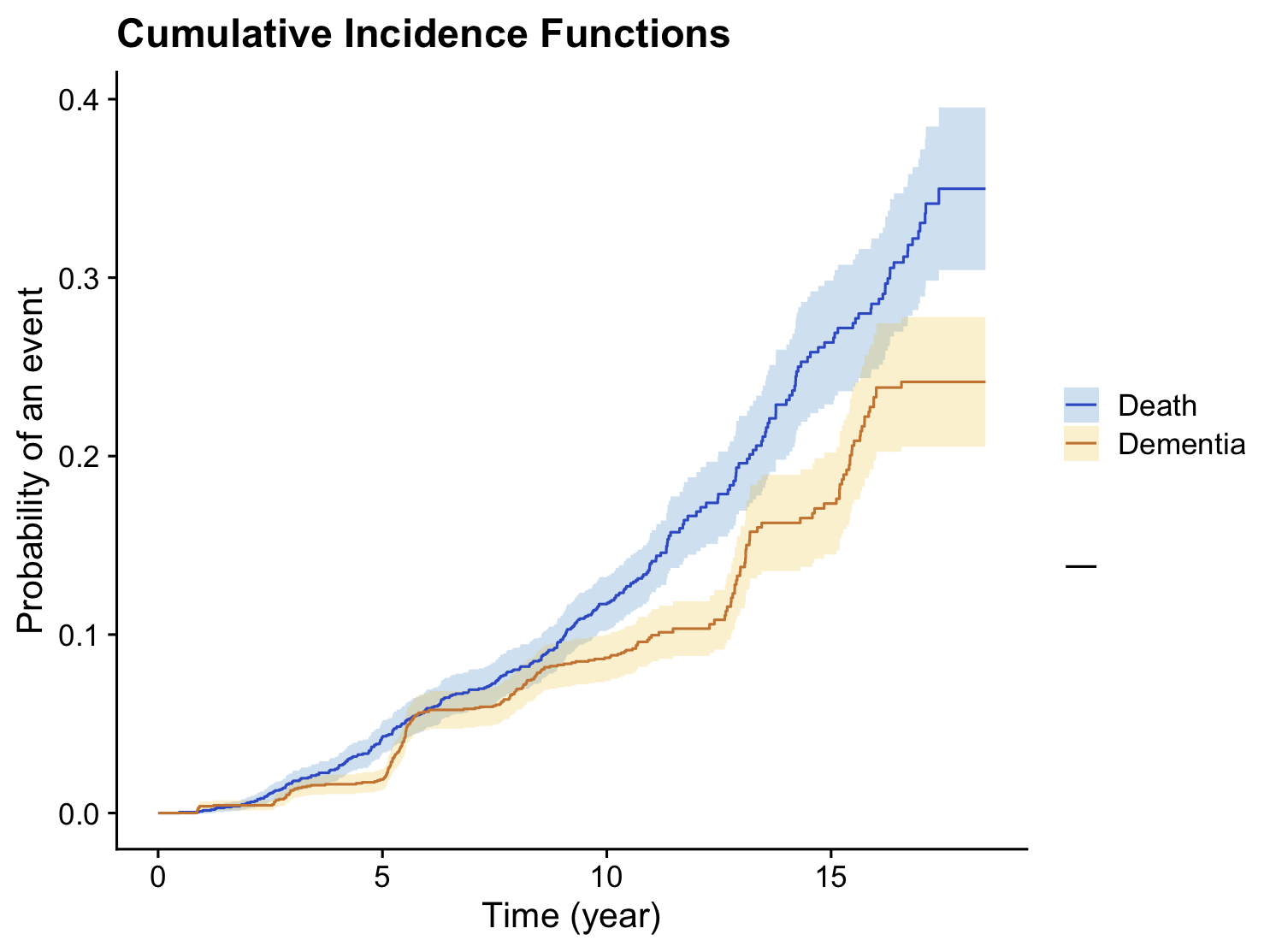
We considered subjects who were dementia-free at the beginning of the study and had at least one measurement for each of the longitudinal markers. Out of these subjects, 227 were diagnosed with incident dementia, and 311 died before
developing dementia. Figure A.1 shows the cumulative incidence function for dementia and death in this sample.
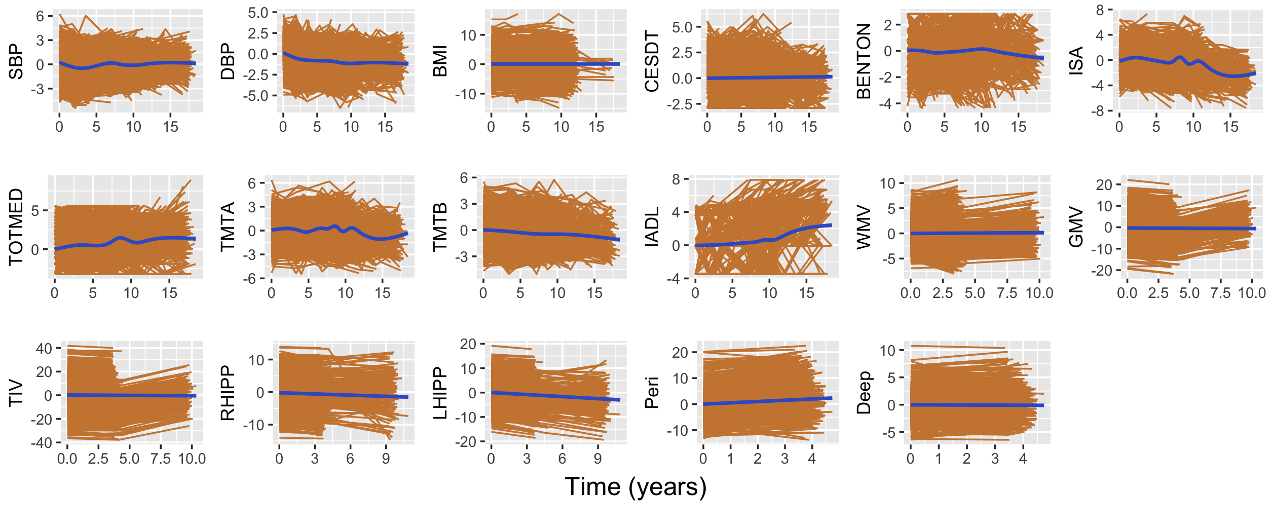
We considered seventeen longitudinal markers: three cardio-metabolic markers (body mass index (BMI), diastolic blood pressure (DBP), and systolic blood pressure (SBP)), the total number of medications (TOTMED), depressive symptomatology measured using the Center for Epidemiologic Studies-Depression scale (CESDT, the lower the better), functional dependency assessed using the Instrumental Activities of Daily Living scale (IADL, the lower the better), four cognitive tests (the visual retention test of Benton (BENTON, number of correct responses out of 15), the Isaacs set test (ISA, total number of words given in 4 semantic categories in 15 seconds), the trail making tests A and B (TMTA and TMTB, number of correct moves per minute), the total intracranial volume (TIV), and some biomarkers of neurodegeneration, including white matter volume (WMV), gray matter volume (GMV), left hippocampal volume (LHIPP), and right hippocampal volume (RHIPP); two markers of vascular brain lesions including the volumes of white matter hyperintensities in the periventricular (Peri), and deep (Deep) white matter.
Figure A.2 shows individual trajectories of the longitudinal markers in the 3C study, illustrating time-dependent variables. The data were pre-transformed using splines to satisfy the normality assumption of linear mixed models
[16].
The minimum, maximum, and median number of repeated measurements for SBP, DBP, CESDT, BENTON, ISA, TOTMED, and IADL are 1, 8, and 5, respectively. For BMI, TMTA, and TMTB, the minimum, maximum, and median number of repeated measurements are 1, 7, and 4, respectively. The minimum, maximum, and median number of repeated measurements for WMV, GMV, TIV, RHIPP, and LHIPP are 1, 3, and 2, respectively. For Peri and Deep (which were not measured at year 10), there are at most two repeated measures, with a median equal to 2.
In addition, the model incorporates five time-invariant explanatory variables including age at enrollment (), sex (0=male, 1=female), education level (Educ, 0=less than 10 years of schooling, 1=at least 10 years of schooling), Diabetes status at baseline (1=yes), and APOE4 allele carrier status (the main genetic susceptibility factor for Alzheimer’s disease, 1=presence of APOE4).
5.2 Data analysis
For analyzing the 3C data using the proposed approach, we partitioned the dataset into two distinct sets: the training set, comprising 70% of the data, and a separate validation set. Parameter estimation was conducted using the training data, while risk prediction was exclusively performed on the validation set.
For this aim, a quadratic time trend is considered for both fixed and random effects, as a non-linear time trend was previously observed for SBP, DBP, BMI, CESDT, BENTON, ISA, TOTMED, TMTA, TMTB, and IADL [16]:
For other longitudinal markers, a linear mixed model is considered:
To model dementia and death, we utilize proportional hazard models that may depend on the five time-invariant explanatory variables and the current value of the markers. Let denote the cause-specific hazard function for subject , where for dementia and for death. The proportional hazard model takes the following form:
Table A.1 in the supplementary material displays the estimated regression coefficients and variance of error from the mixed effects sub-models for each marker in the one-marker joint models. Additionally, Table 5 presents the estimated parameters from the proportional hazard models for dementia and death, considering the VSJM approach given you choose DS, this is an additional reason for not emphasizing on a vague superiority of CS which is debatable in the simulation results, including estimates, standard deviations, credible intervals, lBFDRs, and BFs (left part). Subsequently, the right part presents the estimates obtained after re-estimating the model with non-informative priors including only the significant variables selected variables according to lBFDR and BF.
The analysis identifies several significant factors associated with dementia and death.
Specifically, high TIV and IADL values, coupled with lower scores on the BENTON, ISA, and TMTB tests, are linked to an increased risk of dementia. Additionally, higher educational attainment, when adjusted for current cognitive scores, is also associated with a higher risk of dementia.
For death without dementia, lower DBP and BENTON scores, increasing age, diabetes, and high educational levels (adjusted for current cognitive scores) are associated with a higher risk. Conversely, being female are linked to a lower risk of death. The results for CS remains similar, and are reported in Table A.2.
The predictive abilities of the model for the years prediction of dementia accounting for the competing risk of death were assessed at landmark times and years. To avoid overoptimistic results, AUC and BS were computed on a validation set.
The predictive abilities presented in table 6 are very good. The AUC is always higher than 0.9 except for s=0 with CS and BF and higher for and compared to , highlighting the information brought by the repeated measures of the longitudinal markers. Results were very similar for CS and DS priors and slightly better for LBFDR compared to BF.
| VSJM | Re-estimation (LBFDR) | Re-estimation (BF) | ||||||||||||
|---|---|---|---|---|---|---|---|---|---|---|---|---|---|---|
| Est. | SD | CI | CI | lBFDR | BF | Est. | SD | CI | CI | Est. | SD | CI | CI | |
| Dementia | ||||||||||||||
| WMV | 0.000 | 0.000 | 0.000 | 0.000 | 1.000 | 0.000 | ||||||||
| GMV | 0.000 | 0.000 | 0.000 | 0.000 | 1.000 | 0.000 | ||||||||
| TIV | 0.060 | 0.010 | 0.040 | 0.079 | 0.000 | Inf | 0.059 | 0.010 | 0.040 | 0.079 | 0.059 | 0.010 | 0.040 | 0.078 |
| RHIPP | 0.000 | 0.000 | 0.000 | 0.000 | 1.000 | 0.000 | ||||||||
| LHIPP | -0.079 | 0.018 | -0.115 | -0.043 | 0.000 | Inf | -0.078 | 0.019 | -0.115 | -0.042 | -0.079 | 0.018 | -0.114 | -0.044 |
| Peri | 0.000 | 0.000 | 0.000 | 0.000 | 1.000 | 0.000 | ||||||||
| Deep | 0.000 | 0.000 | 0.000 | 0.000 | 1.000 | 0.000 | ||||||||
| SBP | 0.000 | 0.000 | 0.000 | 0.000 | 1.000 | 0.000 | ||||||||
| DBP | 0.000 | 0.000 | 0.000 | 0.000 | 1.000 | 0.000 | ||||||||
| BMI | -0.018 | 0.034 | -0.103 | 0.000 | 0.765 | 0.308 | ||||||||
| CESDT | 0.013 | 0.043 | 0.000 | 0.171 | 0.900 | 0.111 | ||||||||
| BENTON | -0.500 | 0.119 | -0.744 | -0.272 | 0.000 | Inf | -0.500 | 0.112 | -0.717 | -0.265 | -0.510 | 0.108 | -0.723 | -0.295 |
| ISA | -0.323 | 0.079 | -0.469 | -0.171 | 0.000 | Inf | -0.321 | 0.075 | -0.474 | -0.180 | -0.311 | 0.078 | -0.468 | -0.168 |
| TOTMED | 0.000 | 0.000 | 0.000 | 0.000 | 1.000 | 0.000 | ||||||||
| TMTA | 0.000 | 0.000 | 0.000 | 0.000 | 1.000 | 0.000 | ||||||||
| TMTB | -1.140 | 0.110 | -1.345 | -0.930 | 0.000 | Inf | -1.150 | 0.104 | -1.345 | -0.946 | -1.150 | 0.102 | -1.346 | -0.953 |
| IADL | 0.326 | 0.062 | 0.207 | 0.445 | 0.000 | Inf | 0.333 | 0.058 | 0.222 | 0.450 | 0.329 | 0.057 | 0.220 | 0.444 |
| Sex | 0.002 | 0.028 | 0.000 | 0.000 | 0.986 | 0.014 | ||||||||
| Diabete | 0.000 | 0.025 | 0.000 | 0.000 | 0.996 | 0.004 | ||||||||
| APOE | 0.002 | 0.032 | 0.000 | 0.000 | 0.994 | 0.006 | ||||||||
| Educ | 0.891 | 0.186 | 0.536 | 1.245 | 0.000 | Inf | 0.913 | 0.175 | 0.560 | 1.253 | 0.914 | 0.177 | 0.563 | 1.259 |
| Age | 0.000 | 0.000 | 0.000 | 0.000 | 1.000 | 0.000 | ||||||||
| Death | ||||||||||||||
| WMV | 0.000 | 0.000 | 0.000 | 0.000 | 1.000 | 0.000 | ||||||||
| GMV | 0.000 | 0.000 | 0.000 | 0.000 | 1.000 | 0.000 | ||||||||
| TIV | 0.000 | 0.000 | 0.000 | 0.000 | 1.000 | 0.000 | ||||||||
| RHIPP | 0.000 | 0.000 | 0.000 | 0.000 | 1.000 | 0.000 | ||||||||
| LHIPP | 0.000 | 0.000 | 0.000 | 0.000 | 1.000 | 0.000 | ||||||||
| Peri | 0.000 | 0.000 | 0.000 | 0.000 | 1.000 | 0.000 | ||||||||
| Deep | 0.000 | 0.000 | 0.000 | 0.000 | 1.000 | 0.000 | ||||||||
| SBP | 0.000 | 0.000 | 0.000 | 0.000 | 1.000 | 0.000 | ||||||||
| DBP | -0.155 | 0.048 | -0.248 | -0.060 | 0.000 | Inf | -0.154 | 0.047 | -0.245 | -0.059 | -0.156 | 0.046 | -0.246 | -0.065 |
| BMI | 0.000 | 0.000 | 0.000 | 0.000 | 1.000 | 0.000 | ||||||||
| CESDT | 0.000 | 0.000 | 0.000 | 0.000 | 1.000 | 0.000 | ||||||||
| BENTON | -3.347 | 0.132 | -3.623 | -3.097 | 0.000 | Inf | -3.365 | 0.150 | -3.643 | -3.081 | -3.313 | 0.154 | -3.618 | -3.021 |
| ISA | 0.000 | 0.000 | 0.000 | 0.000 | 1.000 | 0.000 | ||||||||
| TOTMED | 0.000 | 0.000 | 0.000 | 0.000 | 1.000 | 0.000 | ||||||||
| TMTA | 0.000 | 0.000 | 0.000 | 0.000 | 1.000 | 0.000 | ||||||||
| TMTB | 0.000 | 0.000 | 0.000 | 0.000 | 1.000 | 0.000 | ||||||||
| IADL | 0.000 | 0.000 | 0.000 | 0.000 | 1.000 | 0.000 | ||||||||
| Sex | -2.200 | 0.175 | -2.553 | -1.872 | 0.000 | Inf | -2.215 | 0.175 | -2.555 | -1.865 | -2.184 | 0.179 | -2.514 | -1.828 |
| Diabete | 1.046 | 0.183 | 0.677 | 1.398 | 0.000 | Inf | 1.062 | 0.194 | 0.683 | 1.442 | 1.039 | 0.187 | 0.685 | 1.401 |
| APOE | 0.000 | 0.000 | 0.000 | 0.000 | 1.000 | 0.000 | ||||||||
| Educ | 0.870 | 0.159 | 0.548 | 1.178 | 0.000 | Inf | 0.869 | 0.155 | 0.558 | 1.182 | 0.854 | 0.151 | 0.563 | 1.142 |
| Age | 1.230 | 0.191 | 0.844 | 1.588 | 0.000 | Inf | 1.255 | 0.192 | 0.875 | 1.628 | 1.216 | 0.188 | 0.841 | 1.589 |
| lBFDR | BF | ||||||||
|---|---|---|---|---|---|---|---|---|---|
| AUC | BS | AUC | BS | ||||||
| Est. | SD. | Est. | SD. | Est. | SD. | Est. | SD. | ||
| DS | |||||||||
| 0.891 | 0.037 | 0.019 | 0.005 | 0.885 | 0.034 | 0.019 | 0.005 | ||
| 0.891 | 0.018 | 0.130 | 0.014 | 0.846 | 0.027 | 0.152 | 0.016 | ||
| 0.971 | 0.016 | 0.044 | 0.016 | 0.901 | 0.035 | 0.122 | 0.029 | ||
| CS | |||||||||
| 0.731 | 0.070 | 0.058 | 0.006 | 0.827 | 0.075 | 0.020 | 0.004 | ||
| 0.851 | 0.022 | 0.184 | 0.016 | 0.895 | 0.017 | 0.109 | 0.012 | ||
| 0.863 | 0.045 | 0.135 | 0.028 | 0.945 | 0.023 | 0.086 | 0.022 | ||
6 Conclusion
In this paper, we introduce a novel approach for variable selection in joint modeling for multiple longitudinal markers and competing risks outcomes in a Bayesian paradigm.
Our method utilizes a spike and slab prior for the association parameters and regression coefficients in the survival model. The approach involves two key steps: initially, a simple Bayesian joint modeling of each longitudinal marker and competing risks outcome is conducted, followed by variable selection using a time-dependent Bayesian proportional hazard model. This model incorporates Dirac spike or continuous spike priors for regression coefficients, including those for time-dependent markers and fixed covariates. We also propose two criteria, namely Bayes factor and local Bayesian false discovery rate, for making final decisions in variable selection.
In addition to variable selection, our paper explores dynamic prediction based on the estimated joint model. To achieve this, we suggest re-estimating the second step of the approach, taking into account the selected markers and covariates.
We evaluate the performance of our approach through extensive simulation studies, focusing on variable selection and dynamic prediction. Furthermore, we apply our proposed method to analyze and predict the risk of dementia using the 3C dataset. The implementation of our method is available in the freely accessible R package VSJM, which can be found at https://github.com/tbaghfalaki/VSJM.
As a future direction, our approach can be extended to accommodate non Gaussian longitudinal markers by including generalised linear mixed sub-model in the one-marker joint models.
Moreover, while we focus on variable selection in this work, there is potential to extend our approach to group selection, offering further flexibility and applicability.
Declarations
Ethics approval and consent to participate
Not applicable.
Consent for publication
Not applicable.
Availability of data and materials
To facilitate implementation, we introduce an R package called VSJM, which is freely available at https://github.com/tbaghfalaki/VSJM. Vignette and example usage is available at https://github.com/tbaghfalaki/VSJM/blob/main/Exam1.md.
Competing interests
Not applicable.
Funding
Not applicable
Authors’ contributions
HJG and TB conceptualized and designed the study. CT and CH provided the data, while HJG and TB performed the data analysis and interpretation. HJG, TB, and RH developed the simulation studies. TB wrote the R code. All authors contributed to the manuscript preparation, reviewed, and approved the final version.
Acknowledgements
This work was partly funded by the French National Research Agency (grant ANR-21-CE36 for the project “Joint Models for Epidemiology and Clinical research”). This study received financial support from the French government in the framework of the University of Bordeaux’s IdEx ”Investments for the Future” program / RRI PHDS. The 3C Study was supported by Sanofi-Synthélabo, the FRM, the CNAM-TS,DGS,Conseils Régionaux of Aquitaine, 395 Languedoc-Roussillon, and Bourgogne; Foundation of France; Ministry of Research- INSERM “Cohorts and biological data collections” program; MGEN; Longevity Institute; General Council of the Côte d’Or; ANR PNRA 2006 (grant ANR/ DEDD/ PNRA/ PROJ/ 200206–01-01) and Longvie 2007 (grant LVIE-003-01); Alzheimer Plan Foundation (FCS grant 2009-2012); and Roche. The Three City Study data are available upon request at e3c.coordinatingcenter@gmail.com.
References
- [1] Maha Alsefri, Maria Sudell, Marta García-Fiñana, and Ruwanthi Kolamunnage-Dona. Bayesian joint modelling of longitudinal and time to event data: a methodological review. BMC medical research methodology, 20:1–17, 2020.
- [2] Marilyn Antoniak, Maura Pugliatti, Richard Hubbard, John Britton, Stefano Sotgiu, A Dessa Sadovnick, Irene ML Yee, Miguel A Cumsille, Jorge A Bevilacqua, Sarah Burdett, et al. Vascular factors and risk of dementia: design of the three-city study and baseline characteristics of the study population. Neuroepidemiology, 22(6):316–325, 2003.
- [3] Peter C Austin. Generating survival times to simulate cox proportional hazards models with time-varying covariates. Statistics in medicine, 31(29):3946–3958, 2012.
- [4] Taban Baghfalaki, Mojtaba Ganjali, and Damon Berridge. Joint modeling of multivariate longitudinal mixed measurements and time to event data using a bayesian approach. Journal of Applied Statistics, 41(9):1934–1955, 2014.
- [5] Taban Baghfalaki, Reza Hashemi, Catherine Helmer, and Helene Jacqmin-Gadda. A two-stage joint modeling approach for multiple longitudinal markers and time-to-event data. submitted, pages 1–33, 2024.
- [6] Taban Baghfalaki, Pierre-Emmanuel Sugier, Therese Truong, Anthony N Pettitt, Kerrie Mengersen, and Benoit Liquet. Bayesian meta-analysis models for cross cancer genomic investigation of pleiotropic effects using group structure. Statistics in Medicine, 40(6):1498–1518, 2021.
- [7] Yoav Benjamini and Yosef Hochberg. Controlling the false discovery rate: a practical and powerful approach to multiple testing. Journal of the Royal statistical society: series B (Methodological), 57(1):289–300, 1995.
- [8] Paul Blanche, Cécile Proust-Lima, Lucie Loubère, Claudine Berr, Jean-François Dartigues, and Hélène Jacqmin-Gadda. Quantifying and comparing dynamic predictive accuracy of joint models for longitudinal marker and time-to-event in presence of censoring and competing risks. Biometrics, 71(1):102–113, 2015.
- [9] Ignace Bogaert. Iteration-free computation of gauss–legendre quadrature nodes and weights. SIAM Journal on Scientific Computing, 36(3):A1008–A1026, 2014.
- [10] Sam Brilleman. Estimating joint models for longitudinal and time-to-event data with rstanarm. https://cran.uni-muenster.de/web/packages/rstanarm/vignettes/jm.html, 2023.
- [11] Peter Bühlmann and Sara Van De Geer. Statistics for high-dimensional data: methods, theory and applications. Springer Science & Business Media, Germany, 2011.
- [12] Carlos M Carvalho, Nicholas G Polson, and James G Scott. The horseshoe estimator for sparse signals. Biometrika, 97(2):465–480, 2010.
- [13] Yuqi Chen and Yuedong Wang. Variable selection for joint models of multivariate longitudinal measurements and event time data. Statistics in medicine, 36(24):3820–3829, 2017.
- [14] Yueh-Yun Chi and Joseph G Ibrahim. Joint models for multivariate longitudinal and multivariate survival data. Biometrics, 62(2):432–445, 2006.
- [15] Mohammad Ziaul Islam Chowdhury and Tanvir C Turin. Variable selection strategies and its importance in clinical prediction modelling. Family medicine and community health, 8(1), 2020.
- [16] Anthony Devaux, Catherine Helmer, Carole Dufouil, Robin Genuer, and Cécile Proust-Lima. Random survival forests for competing risks with multivariate longitudinal endogenous covariates. arXiv preprint arXiv:2208.05801, 2022.
- [17] Bradley Efron. Large-scale simultaneous hypothesis testing: the choice of a null hypothesis. Journal of the American Statistical Association, 99(465):96–104, 2004.
- [18] Bradley Efron. Large-scale inference: empirical Bayes methods for estimation, testing, and prediction, volume 1. Cambridge University Press, United Kingdom, 2012.
- [19] Bradley Efron, Alan Gous, RE Kass, GS Datta, and P Lahiri. Scales of evidence for model selection: Fisher versus jeffreys. Lecture Notes-Monograph Series, pages 208–256, 2001.
- [20] Bradley Efron and Robert Tibshirani. Empirical bayes methods and false discovery rates for microarrays. Genetic epidemiology, 23(1):70–86, 2002.
- [21] Andrew Gelman, John B Carlin, Hal S Stern, and Donald B Rubin. Bayesian data analysis. Chapman and Hall/CRC, United States, 1995.
- [22] Edward I George and Robert E McCulloch. Variable selection via gibbs sampling. Journal of the American Statistical Association, 88(423):881–889, 1993.
- [23] Colin Griesbach, Andreas Mayr, and Elisabeth Bergherr. Variable selection and allocation in joint models via gradient boosting techniques. Mathematics, 11(2):411, 2023.
- [24] Jeremie Guedj, Rodolphe Thiébaut, and Daniel Commenges. Joint modeling of the clinical progression and of the biomarkers’ dynamics using a mechanistic model. Biometrics, 67(1):59–66, 2011.
- [25] Zangdong He, Wanzhu Tu, Sijian Wang, Haoda Fu, and Zhangsheng Yu. Simultaneous variable selection for joint models of longitudinal and survival outcomes. Biometrics, 71(1):178–187, 2015.
- [26] Md Akhtar Hossain. Multivariate Joint Models and Dynamic Predictions. PhD thesis, University of South Carolina, 2020.
- [27] Joseph G Ibrahim, Ming-Hui Chen, Debajyoti Sinha, JG Ibrahim, and MH Chen. Bayesian survival analysis, volume 2. Springer, Germany, 2001.
- [28] Robert E Kass and Adrian E Raftery. Bayes factors. Journal of the american statistical association, 90(430):773–795, 1995.
- [29] Jeffrey Lin and Sheng Luo. Deep learning for the dynamic prediction of multivariate longitudinal and survival data. Statistics in medicine, 41(15):2894–2907, 2022.
- [30] Jeffrey D Long and James A Mills. Joint modeling of multivariate longitudinal data and survival data in several observational studies of huntington’s disease. BMC medical research methodology, 18(1):1–15, 2018.
- [31] Arunabha Majumdar, Tanushree Haldar, Sourabh Bhattacharya, and John S Witte. An efficient bayesian meta-analysis approach for studying cross-phenotype genetic associations. PLoS genetics, 14(2):e1007139, 2018.
- [32] Gertraud Malsiner-Walli and Helga Wagner. Comparing spike and slab priors for bayesian variable selection. Austrian Journal of Statistics, 40(4):241–264, 2011.
- [33] B.W. Matthews. Comparison of the predicted and observed secondary structure of t4 phage lysozyme. Biochimica et Biophysica Acta (BBA) - Protein Structure, 405(2):442 – 451, 1975.
- [34] Toby J Mitchell and John J Beauchamp. Bayesian variable selection in linear regression. Journal of the american statistical association, 83(404):1023–1032, 1988.
- [35] Grigorios Papageorgiou, Katya Mauff, Anirudh Tomer, and Dimitris Rizopoulos. An overview of joint modeling of time-to-event and longitudinal outcomes. Annual review of statistics and its application, 6:223–240, 2019.
- [36] Martyn Plummer. Jags version 3.3. 0 user manual. International Agency for Research on Cancer, Lyon, France, 2012.
- [37] Martyn Plummer et al. Jags: A program for analysis of bayesian graphical models using gibbs sampling. In Proceedings of the 3rd international workshop on distributed statistical computing, volume 124, pages 1–10. Vienna, Austria, 2003.
- [38] D Rizopoulos, G Papageorgiou, and P Miranda Afonso. Jmbayes2: extended joint models for longitudinal and time-to-event data. R package version 0.2-4, 2022.
- [39] Dimitris Rizopoulos. Dynamic predictions and prospective accuracy in joint models for longitudinal and time-to-event data. Biometrics, 67(3):819–829, 2011.
- [40] Dimitris Rizopoulos. Joint models for longitudinal and time-to-event data: With applications in R. CRC press, New York, 2012.
- [41] Dimitris Rizopoulos. The r package jmbayes for fitting joint models for longitudinal and time-to-event data using mcmc. Journal of Statistical Software, 72:1–46, 2016.
- [42] Dimitris Rizopoulos and Pulak Ghosh. A bayesian semiparametric multivariate joint model for multiple longitudinal outcomes and a time-to-event. Statistics in medicine, 30(12):1366–1380, 2011.
- [43] Sheldon M Ross. Simulation, 5th edision, 2012.
- [44] Denis Rustand, Elias T Krainski, and Haavard Rue. Denisrustand/inlajoint: Joint modeling multivariate longitudinal and time-to-event outcomes with inla. https://repository.kaust.edu.sa/items/82751567-82c6-477e-92af-8a2e9a7b0c3b, 2022.
- [45] Joshua N Sampson, Nilanjan Chatterjee, Raymond J Carroll, and Samuel Müller. Controlling the local false discovery rate in the adaptive lasso. Biostatistics, 14(4):653–666, 2013.
- [46] James G Scott and James O Berger. Bayes and empirical-bayes multiplicity adjustment in the variable-selection problem. The Annals of Statistics, pages 2587–2619, 2010.
- [47] Fan Shen and Liang Li. Backward joint model and dynamic prediction of survival with multivariate longitudinal data. Statistics in medicine, 40(20):4395–4409, 2021.
- [48] Xiao Song, Marie Davidian, and Anastasios A Tsiatis. An estimator for the proportional hazards model with multiple longitudinal covariates measured with error. Biostatistics, 3(4):511–528, 2002.
- [49] Inês Sousa. A review on joint modelling of longitudinal measurements and time-to-even. REVSTAT-Statistical Journal, 9(1):57–81, 2011.
- [50] Ewout W Steyerberg. Applications of prediction models. In Clinical prediction models, pages 11–31. Springer, Germany, 2009.
- [51] Yu-Sung Su and Masanao Yajima. R2jags: Using r to run ‘jags’. R package version 0.5-7, 34, 2015.
- [52] An-Min Tang, Xingqiu Zhao, and Nian-Sheng Tang. Bayesian variable selection and estimation in semiparametric joint models of multivariate longitudinal and survival data. Biometrical Journal, 59(1):57–78, 2017.
- [53] Jiarui Tang, An-Min Tang, and Niansheng Tang. Variable selection for joint models of multivariate skew-normal longitudinal and survival data. Statistical Methods in Medical Research, 32(9):1694–1710, 2023.
- [54] James Tanton. Encyclopedia of mathematics. Facts On File, Inc, United States, 2005.
- [55] Peter M Williams. Bayesian regularization and pruning using a laplace prior. Neural computation, 7(1):117–143, 1995.
- [56] Yujing Xie, Zangdong He, Wanzhu Tu, and Zhangsheng Yu. Variable selection for joint models with time-varying coefficients. Statistical Methods in Medical Research, 29(1):309–322, 2020.
- [57] Jane Xu and Scott L Zeger. The evaluation of multiple surrogate endpoints. Biometrics, 57(1):81–87, 2001.
- [58] Xiaofan Xu, Malay Ghosh, et al. Bayesian variable selection and estimation for group lasso. Bayesian Analysis, 10(4):909–936, 2015.
- [59] Jurel K Yap and Iris Ivy M Gauran. Bayesian variable selection using knockoffs with applications to genomics. Computational Statistics, 38(4):1771–1790, 2023.
- [60] Fengting Yi, Niansheng Tang, and Jianguo Sun. Simultaneous variable selection and estimation for joint models of longitudinal and failure time data with interval censoring. Biometrics, 78(1):151–164, 2022.
- [61] TianHong Zhang, XiaoChen Tang, Yue Zhang, LiHua Xu, YanYan Wei, YeGang Hu, HuiRu Cui, YingYing Tang, HaiChun Liu, Tao Chen, et al. Multivariate joint models for the dynamic prediction of psychosis in individuals with clinical high risk. Asian Journal of Psychiatry, 81:103468, 2023.
- [62] Xiang Zhou and Jerome P Reiter. A note on bayesian inference after multiple imputation. The American Statistician, 64(2):159–163, 2010.
- [63] Kirill Zhudenkov, Sergey Gavrilov, Alina Sofronova, Oleg Stepanov, Nataliya Kudryashova, Gabriel Helmlinger, and Kirill Peskov. A workflow for the joint modeling of longitudinal and event data in the development of therapeutics: Tools, statistical methods, and diagnostics. CPT: Pharmacometrics & Systems Pharmacology, 11(4):425–437, 2022.
Supplementary Material
| Est. | SD | CI | CI | ||
| WMV | Intercept | -0.004 | 0.063 | -0.119 | 0.114 |
| Time | 0.027 | 0.012 | 0.004 | 0.051 | |
| 0.765 | 0.063 | 0.629 | 0.875 | ||
| GMV | Intercept | -0.102 | 0.145 | -0.382 | 0.170 |
| Time | -0.246 | 0.021 | -0.285 | -0.205 | |
| 1.994 | 0.107 | 1.797 | 2.216 | ||
| TIV | Intercept | -0.293 | 0.299 | -0.779 | 0.420 |
| Time | 0.019 | 0.028 | -0.037 | 0.074 | |
| 3.760 | 0.199 | 3.394 | 4.168 | ||
| RHIPP | Intercept | 0.137 | 0.100 | -0.042 | 0.327 |
| Time | -0.316 | 0.013 | -0.340 | -0.291 | |
| 0.905 | 0.054 | 0.801 | 1.018 | ||
| LHIPP | Intercept | 0.087 | 0.112 | -0.128 | 0.297 |
| Time | -0.350 | 0.014 | -0.379 | -0.322 | |
| 1.017 | 0.062 | 0.900 | 1.144 | ||
| Peri | Intercept | -0.074 | 0.116 | -0.310 | 0.132 |
| Time | 0.605 | 0.029 | 0.549 | 0.661 | |
| 1.704 | 0.493 | 0.945 | 2.671 | ||
| Deep | Intercept | -0.009 | 0.058 | -0.120 | 0.108 |
| Time | 0.019 | 0.012 | -0.004 | 0.043 | |
| 0.601 | 0.097 | 0.394 | 0.770 | ||
| SBP | Intercept | 0.053 | 0.085 | -0.071 | 0.198 |
| Time | -0.327 | 0.286 | -0.668 | -0.027 | |
| Time2 | 0.064 | 0.071 | -0.008 | 0.140 | |
| 0.994 | 0.037 | 0.934 | 1.072 | ||
| DBP | Intercept | -0.038 | 0.108 | -0.179 | 0.118 |
| Time | -0.488 | 0.339 | -0.863 | -0.135 | |
| Time2 | 0.075 | 0.084 | -0.010 | 0.162 | |
| 0.967 | 0.040 | 0.907 | 1.062 | ||
| BMI | Intercept | 0.014 | 0.225 | -0.273 | 0.299 |
| Time | 0.015 | 0.047 | -0.057 | 0.079 | |
| Time2 | 0.003 | 0.017 | -0.015 | 0.022 | |
| 0.997 | 0.044 | 0.933 | 1.100 | ||
| CESDT | Intercept | 0.053 | 0.163 | -0.160 | 0.258 |
| Time | -0.060 | 0.196 | -0.305 | 0.150 | |
| Time2 | 0.011 | 0.054 | -0.044 | 0.070 | |
| 1.029 | 0.028 | 0.981 | 1.091 | ||
| BENTON | Intercept | 0.110 | 0.063 | 0.010 | 0.235 |
| Time | -0.239 | 0.223 | -0.517 | 0.000 | |
| Time2 | 0.049 | 0.053 | -0.005 | 0.107 | |
| 0.980 | 0.030 | 0.925 | 1.037 | ||
| ISA | Intercept | 0.069 | 0.113 | -0.079 | 0.251 |
| Time | -0.143 | 0.229 | -0.436 | 0.109 | |
| Time2 | 0.029 | 0.051 | -0.023 | 0.085 | |
| 0.963 | 0.027 | 0.911 | 1.017 | ||
| TOTMED | Intercept | -0.096 | 0.118 | -0.264 | 0.061 |
| Time | -0.038 | 0.327 | -0.426 | 0.304 | |
| Time2 | 0.038 | 0.077 | -0.041 | 0.121 | |
| 1.053 | 0.046 | 0.977 | 1.140 | ||
| TMTA | Intercept | 0.044 | 0.033 | -0.021 | 0.104 |
| Time | -0.193 | 0.245 | -0.500 | 0.067 | |
| Time2 | 0.051 | 0.057 | -0.007 | 0.113 | |
| 0.957 | 0.049 | 0.879 | 1.058 | ||
| TMTB | Intercept | -0.000 | 0.035 | -0.068 | 0.069 |
| Time | -0.250 | 0.205 | -0.492 | -0.031 | |
| Time2 | 0.040 | 0.054 | -0.015 | 0.098 | |
| 0.975 | 0.052 | 0.893 | 1.091 | ||
| IADL | Intercept | 0.015 | 0.123 | -0.144 | 0.180 |
| Time | -0.055 | 0.089 | -0.175 | 0.050 | |
| Time2 | 0.020 | 0.025 | -0.006 | 0.048 | |
| 0.969 | 0.032 | 0.915 | 1.038 |
| VSJM | Re-estimation (LBFDR) | Re-estimation (BF) | ||||||||||||
|---|---|---|---|---|---|---|---|---|---|---|---|---|---|---|
| Est. | SD | CI | CI | lBFDR | BF | Est. | SD | CI | CI | Est. | SD | CI | CI | |
| Dementia | ||||||||||||||
| WMV | -0.030 | 0.022 | -0.076 | 0.008 | 0.991 | 0.009 | ||||||||
| GMV | 0.009 | 0.019 | -0.029 | 0.042 | 1.000 | 0.000 | ||||||||
| TIV | 0.033 | 0.011 | 0.011 | 0.053 | 1.000 | 0.000 | ||||||||
| RHIPP | -0.020 | 0.019 | -0.055 | 0.015 | 1.000 | 0.000 | ||||||||
| LHIPP | -0.042 | 0.021 | -0.085 | -0.001 | 1.000 | 0.000 | ||||||||
| Peri | 0.021 | 0.015 | -0.005 | 0.053 | 1.000 | 0.000 | ||||||||
| Deep | 0.020 | 0.026 | -0.037 | 0.065 | 1.000 | 0.000 | ||||||||
| SBP | -0.006 | 0.040 | -0.078 | 0.062 | 0.988 | 0.012 | ||||||||
| DBP | -0.041 | 0.032 | -0.102 | 0.020 | 1.000 | 0.000 | ||||||||
| BMI | -0.003 | 0.014 | -0.032 | 0.027 | 1.000 | 0.000 | ||||||||
| CESDT | 0.038 | 0.030 | -0.022 | 0.100 | 1.000 | 0.000 | ||||||||
| BENTON | -0.893 | 0.187 | -1.251 | -0.604 | 0.000 | Inf | -1.201 | 0.085 | -1.366 | -1.038 | -0.783 | 0.096 | -0.969 | -0.590 |
| ISA | -0.034 | 0.031 | -0.094 | 0.027 | 1.000 | 0.000 | ||||||||
| TOTMED | -0.040 | 0.033 | -0.107 | 0.019 | 1.000 | 0.000 | ||||||||
| TMTA | 0.004 | 0.042 | -0.077 | 0.074 | 1.000 | 0.000 | ||||||||
| TMTB | -0.851 | 0.489 | -1.344 | -0.079 | 0.297 | 2.364 | -1.235 | 0.094 | -1.412 | -1.045 | ||||
| IADL | 0.440 | 0.089 | 0.296 | 0.623 | 0.000 | Inf | 0.625 | 0.056 | 0.518 | 0.735 | 0.382 | 0.055 | 0.278 | 0.490 |
| Sex | -0.001 | 0.032 | -0.062 | 0.061 | 1.000 | 0.000 | ||||||||
| Diabete | 0.009 | 0.054 | -0.054 | 0.071 | 0.979 | 0.021 | ||||||||
| APOE | 0.688 | 0.183 | 0.311 | 1.020 | 0.000 | Inf | 0.897 | 0.174 | 0.548 | 1.225 | 0.737 | 0.179 | 0.380 | 1.084 |
| Educ | 0.641 | 0.175 | 0.283 | 0.951 | 0.000 | Inf | 0.674 | 0.174 | 0.339 | 1.026 | 0.804 | 0.171 | 0.462 | 1.136 |
| Age | 0.005 | 0.049 | -0.063 | 0.082 | 0.955 | 0.047 | ||||||||
| Death | ||||||||||||||
| WMV | 0.016 | 0.023 | -0.030 | 0.061 | 1.000 | 0.000 | ||||||||
| GMV | -0.010 | 0.019 | -0.046 | 0.026 | 1.000 | 0.000 | ||||||||
| TIV | 0.029 | 0.011 | 0.008 | 0.051 | 1.000 | 0.000 | ||||||||
| RHIPP | -0.007 | 0.017 | -0.038 | 0.024 | 1.000 | 0.000 | ||||||||
| LHIPP | 0.018 | 0.018 | -0.015 | 0.052 | 1.000 | 0.000 | ||||||||
| Peri | 0.001 | 0.011 | -0.020 | 0.023 | 1.000 | 0.000 | ||||||||
| Deep | 0.002 | 0.025 | -0.045 | 0.053 | 1.000 | 0.000 | ||||||||
| SBP | 0.004 | 0.028 | -0.051 | 0.057 | 1.000 | 0.000 | ||||||||
| DBP | 0.296 | 0.047 | 0.203 | 0.393 | 0.000 | Inf | 0.356 | 0.046 | 0.268 | 0.451 | 0.358 | 0.049 | 0.266 | 0.456 |
| BMI | 0.012 | 0.010 | -0.008 | 0.031 | 1.000 | 0.000 | ||||||||
| CESDT | -0.003 | 0.025 | -0.050 | 0.050 | 1.000 | 0.000 | ||||||||
| BENTON | -0.088 | 0.030 | -0.152 | -0.032 | 1.000 | 0.000 | ||||||||
| ISA | -1.761 | 0.084 | -1.936 | -1.620 | 0.000 | Inf | -1.772 | 0.078 | -1.931 | -1.621 | -1.759 | 0.091 | -1.935 | -1.589 |
| TOTMED | 0.075 | 0.027 | 0.022 | 0.129 | 1.000 | 0.000 | ||||||||
| TMTA | 0.014 | 0.028 | -0.041 | 0.064 | 1.000 | 0.000 | ||||||||
| TMTB | 0.014 | 0.027 | -0.041 | 0.068 | 1.000 | 0.000 | ||||||||
| IADL | 0.011 | 0.025 | -0.040 | 0.058 | 1.000 | 0.000 | ||||||||
| Sex | -1.816 | 0.196 | -2.088 | -1.813 | 0.000 | Inf | -1.829 | 0.201 | -2.213 | -1.639 | -1.823 | 0.119 | -2.201 | -1.627 |
| Diabete | 0.125 | 0.221 | -0.050 | 0.662 | 0.763 | 0.311 | ||||||||
| APOE | 0.002 | 0.039 | -0.063 | 0.067 | 0.979 | 0.021 | ||||||||
| Educ | 0.001 | 0.032 | -0.062 | 0.067 | 1.000 | 0.000 | ||||||||
| Age | 1.227 | 0.170 | 0.864 | 1.543 | 0.000 | Inf | 1.086 | 0.178 | 0.743 | 1.446 | 1.068 | 0.185 | 0.707 | 1.434 |