A uni-directional optical pulse propagation equation for materials with both electric and magnetic responses
Abstract
I derive uni-directional wave equations for fields propagating in materials with both electric and magnetic dispersion and nonlinearity. The derivation imposes no conditions on the pulse profile except that the material modulates the propagation only slowly: i.e. that loss, dispersion, and nonlinearity have only a small effect over the scale of a wavelength. It also allows a direct term-to-term comparison of the exact bi-directional theory with its approximate uni-directional counterpart.
I Introduction
In the past few years, composite materials (“metamaterials”) that demonstrate both an electric and magnetic response have been the subject of both experimental and theoretical investigation. Often the motivation for this research is the potential for exotic applications: for example, superresolution Pendry (2000), or the possibility of “trapped rainbow” light storage Tsakmakidis et al. (2007). Despite these interesting possibilities, there is also the more basic need for efficient methods for propagating optical pulses in such metamaterials, in particular in one-dimensional (1D) waveguide geometries. Indeed, methods for doing so have already led to interesting predictions (see, e.g., Scalora et al. (2005); Wen et al. (2007); D’Aguanno et al. (2008)). However, these methods, and earlier ones, (e.g. Agrawal (2007); Brabec and Krausz (1997); Geissler et al. (1999); Kinsler and New (2003)) tend to rely on mechanisms such as the introduction of a co-moving frame, and assumptions that the pulse profile has negligible second-order temporal or spatial derivatives. Assuming second-order derivatives are small may well be reasonable, but it means that the pulse profile must remain well behaved. This approximation therefore might well become poorly controlled Kinsler and New (2003); Kinsler (2002), particularly for ultrashort or otherwise ultrawideband pulses, or exotic or extreme material parameters. Ideally we would prefer to make approximations based solely on the material parameters of our device, so as to avoid making assumptions about the state of an ever-changing propagating pulse.
Here I derive 1D wave equations for a waveguide with both electric and magnetic dispersion, and electric and magnetic nonlinearity. I use the directional fields approach Kinsler et al. (2005); Kinsler (2007a), which allows us to directly write down a first-order wave equation for pulse propagation without complicated derivation or approximation. We simply look at the coupled forward and backward wave equations that are a direct re-expression of Maxwell’s curl equations, and substitute in the appropriate dispersion and nonlinearity. I also show separate examples for second- and third-order nonlinearities in both electric and magnetic responses, although the effects can be combined if desired. Note that these directional fields are applicable to more than just pulse propagation, as they have been used to simplify Poynting-vector-based approaches to electromagnetic continuity equations Kinsler et al. (2009).
The derivation makes only a single, well-defined approximation to reduce the bi-directional forward-backward coupled model down to a single first-order wave equation – that of assuming small changes over the scale of a wavelength. This approximation is remarkably robust for all physically realistic parameter values – see Kinsler (2007b) for an analysis focused on nonlinear effects; more general considerations have been dealt with in terms of factorized wave equations Kinsler (2008). The resulting wave equation retains all the usual intuitive and analytical simplicity of ordinary wave propagation equations, unlike the computationally intensive approach of a direct numerical solution of Maxwell’s equations (see, e.g., Yee-1966tap; Flesch-PM-1996prl; Gilles-MV-1999pre; Brabec and Krausz (1997); Tarasishin-MZ-2001oc; Tyrrell-KN-2005jmo).
This paper is structured as follows: Directional fields and their re-expression of the Maxwell curl equations is outlined in Section II, followed by the reduction of the bi-directional wave equation into a uni-directional form in Section III. Section IV shows wave equations for a doubly-nonlinear third-order nonlinearity material, and Section V does the same for a second-order case. In Section VI propagation under the influence of typical metamaterial responses is discussed, and I conclude in Section VII.
II Directional fields
The directional fields approach Kinsler et al. (2005) allows us to write down wave equations for hybrid electromagnetic fields . Note that here I define with an alternate (and more sensible) sign convention than previously. Further, I also allow for more general types of polarization and magnetization in such a way as to provide a simpler presentation. For propagation along the unit vector u, the propagation (curl) equation for is written in the frequency domain as111See derivation in Appendix A.
| (1) |
with
| (2) |
Here the electric response of the material is encoded in two parts: a spatially invariant linear response component , and the remaining contributions (of any type) in . Similarly, the magnetic response is divided up in the same way between and . Generally we will put the entire non-lossy linear response of the medium (i.e. the dispersion) into the reference parameters and , although it may also be convenient to specify only that the product is real (cf. Kinsler-2009pra). All the nonlinear responses and other complications (“corrections”), such as spatial variations in the material parameters, remain in and . As an example, in Kinsler et al. (2005) this approach was applied to second-harmonic generation in a periodically poled dielectric crystal. The time derivatives of these corrections and correspond to bound electric and magnetic currents respectively Kinsler et al. (2009). These and are functions of both fields E and H, i.e. and . If we choose instead to have frequency-independent and , then the remaining linear response can simply be included in and ; in this case the “weak loss and nonlinearity” condition I use later to decouple forward and backward fields would then need to be broadened to include weak dispersion as well (also see Kinsler et al. (2005) for more discussion). However, neither version imposes any requirements on the pulse profile.
It is useful to give a simple example of the directional fields to provide some insight into their nature. In the pure transverse plane-polarized case, with fields propagating along the direction, and frequency-independent (material parameters) permitivitty and permeability , we can write
| (3) | ||||
| (4) |
where this simple definition matches the original proposal of Fleck Fleck (1970).
It is worth considering how reflections arise in this picture based on spatially invariant reference parameters augmented by corrections terms. Leaving aside for now the distinctions between spatially propagated fields and temporally propagated ones (see the discussion in Kinsler (2008)), transition to a new media can be handled in two ways. First, we could map the existing fields onto new ones based on new reference parameters and . Here a pure field would separate into two pieces, one a forward propagating , and the other a “reflected” backward propagating . Second, we might retain the existing reference parameters, and have modified corrections and . These altered correction terms then couple the forward and backward directed fields, inducing the necessary reflection in ; although as a side-effect of our now no longer optimal and , the forward evolving field is made up of coupled and components Kinsler et al. (2005).
II.1 Material response
We define the electric and magnetic material response in the frequency domain, as it greatly simplifies the description of the linear components. Let us chose a reference behaviour given by , and use them to define reference parameters and . Note that these are allowed to have a frequency dependence Kinsler et al. (2005), and that is just the reciprocal of the (reference) speed of light in the medium (i.e. ). We therefore have that the electric displacement and magnetic fields are
| (5) | |||||
| (6) |
To give a specific example, we can define frequency-dependent loss and dispersive corrections by and , along with (e.g.) independent third-order nonlinearities to both the material responses; although any appropriate expression can be used – even magneto-electric or other types. Thus we can write the frequency domain expressions
| (7) | ||||
| (8) |
where takes the Fourier transform (which is necessary because nonlinear effects are defined in the time domain as powers of the field) and denotes a convolution [i.e., ]. If the nonlinearity is time dependent, then the simple type terms can be replaced with the appropriate convolution. In general, it is best to pick subject to the condition that the sizes of and are minimised.
In a double-negative material (with both ) we would get imaginary , changing the complex phase of away from that given by the original E and H. Since this is in the frequency domain, it converts into a phase shift in the time domain, so although imaginary-valued might seem inconvenient, it does not give unphysical results.
III Wave equations
Starting with the vectorial curl equation (1), I first take the 1D, but bi-directional, limit, and describe the approximation necessary to produce a simpler uni-directional form. After this, I discuss how the common transformations used in optical wave equations can be applied in this context. All equations and field quantities are in the frequency () domain, unless explicitly noted otherwise.
III.1 Bi-directional wave equations
Here we set u along the axis without loss of generality, and consider just an polarized wave (i.e., consisting of ). This means we use the component of eqn. (1) with , so that the wave equations for the full spectrum fields , coupled by corrections and are
| (9) |
Following the detailed discussion in Kinsler (2008)222Section III, we say that this wave equation propagates (“steps”) the fields forward along the direction using oppositely directed fields and . These fields can be written as functions of either time or frequency, and pulses they describe therefore evolve (travel) forward or backward in time.
Consider the example case with parameters and , and in eqns. (7) and (8). Defining , we get
| (10) |
Note that even for a frequency-independent choice of the reference parameters and , the reference wave vector retains a (linear) frequency dependence. Also, the dispersion and/or loss parameters are directly related to and respectively, and not to a refractive index or wavevector . This is why there is a factor of associated with their appearance in eqn. (10) and subsequently.
If written in the time domain, these wave equations are seen to propagate the full temporal history of a field forward in space. There, the reference propagation given by becomes a convolution if retains a nontrivial frequency dependence. However, if we expand around a central frequency in powers of , we can instead convert it (in the time domain) into a Taylor series in time derivatives, which is a popular alternative to the frequency domain form used here. However, if implementing a split-step Fourier method of solving these wave equations, dispersion is applied in the frequency domain, so that in general such an expansion is an unnecessary complication.
III.2 Uni-directional approximation
Now we apply the approximation: that the effect of any correction terms is small over propagation distances of one wavelength – or, if you prefer, over time intervals of one optical period. This translates into a weak loss and nonlinearity assumption; and if the correction terms and include dispersion, a weak dispersion assumption is also made. These are rarely very stringent approximations. If and , then a forward has minimal co-propagating Kinsler et al. (2005). Further, the forward field has a wave vector evolving as , but any generated backward component will evolve as . This gives a very rapid relative oscillation , which will quickly average to zero. Nevertheless, although achievable optical nonlinearity coefficients fall well within this approximation, care may need to be taken with the dispersion, particularly if near a band edge or in the vicinity of a narrow resonance.
A directly comparable approximation is treated exhaustively in Kinsler (2008), where although applied to bi-directional factorizations of the second-order wave equation, the physical considerations are exactly the same: Deviations from the reference behaviour over a propagation distance of one wavelength should be small. Note that the slow evolution approximation applied here is not the same as other “slowly varying” types of approximation [e.g., the slowly varying envelope approximation (SVEA)] – although the physical motivation is similar, the approach used here is far less restrictive.
After we apply this weak correction or “slow evolution” approximation, we set the initial value of , and can be sure that it will stay negligible. Thus eqn. (9) for the full spectrum, forward directed field can be written as
| (11) |
Alternatively, we can scale the field so that it has the same units and scaling as the electric field, using . This gives
| (12) |
Note that and , since . In either version of these uni-directional equations, and – the uni-directional (residual) polarization and (residual) magnetization should not be written as functions of the total fields and .
III.3 Modifications
Either of eqns. (11) or (12) by themselves are sufficient to model the propagation of the electric and magnetic fields. However, there are many traditional simplifications which can be applied, and which in other treatments are even sometimes required in order obtain a simple evolution equation. In particular, the various envelope equations Brabec and Krausz (1997); Kinsler and New (2003); Geissler et al. (1999); Scalora and Crenshaw (1994) all use co-moving and/or envelopes as a preparation for discarding inconvenient derivatives: Here such steps are optional extras.
These are all considered in more detail for a factorised wave equation approach in Kinsler (2008), but here I have adapted them for this context.
-
1.
A co-moving frame can now be added, using . This is a simple linear process that causes no extra complications; the leading right-hand side (RHS) term is replaced by , for frame speed . Setting will cancel the phase velocity of the pulse at , not the group velocity.
-
2.
The field can be split up into pieces localized at certain frequencies, as done in descriptions of optical parametric amplifiers or Raman combs (as in, e.g., Kinsler and New (2003, 2004, 2005)). The wave equation can then be separated into one equation for each piece, coupled by the appropriate frequency-matched polarization terms (see, e.g., Kinsler et al. (2006)).
-
3.
A carrier-envelope description of the field can easily be implemented with the usual prescription of Gabor (1946); Boyd (2003) defining an envelope with respect to carrier frequency and wave vector ; this also provides a built-in a co-moving frame . Multiple envelopes centred at different carrier frequencies and wave vectors (, ) can also be used Kinsler et al. (2006); Boyd (2003).
-
4.
Bandwidth restrictions might be added (see below), either to ensure a smooth envelope or to simplify the wave equations; in addition they might be used to separate out or neglect frequency mixing terms or harmonic generation. As it stands, no bandwidth restrictions were applied when deriving eqns. (11) or (12) – there are only the limitations introduced by the dispersion and/or polarization models to consider. Typically we would expand the model parameters to the first few orders about some convenient reference frequency .
-
5.
Mode averaging is where the transverse extent of a propagating beam is not explicitly modeled, but is subsumed into a description of a transverse mode profile; as such it is typically applied to situations involving optical fibres or other waveguides. Thus we could use mode averaging when calculating the effective dispersion or nonlinear parameters. See, for example, Laegsgaard (2007) for a recent approach, which goes beyond a simple addition of a frequency dependence to the “effective area” of the mode, and generalizes the effective area concept itself.
III.4 Diffraction
One important feature lacking in this approach is the handling of transverse effects such as diffraction, although they can be inserted by hand (at least in the paraxial limit) by adding the term to the RHS Kinsler (2007a). However, no treatment of transverse effects has been achieved in a native directional fields description on the basis of the first-order equations – although transverse terms arise naturally in the second-order equation resulting from taking the curl of eqn. (1). Treating nonlinear diffraction Boardman et al. (2000) suffers the same difficulties, although presumably it might be incorporated in an analogous way as to ordinary diffraction.
IV Third-order nonlinearity
Third-order nonlinearities are common in many materials, for example in the silica used to make optical fibres (see, e.g., Agrawal (2007)). There are many applications of significant scientific interest, for example, white light supercontinnua Alfano and Shapiro (1970a, b); Dudley et al. (2006), optical rogue waves Solli et al. (2007); or filamentation Braun et al. (1995); Berge and Skupin (2009).
Here we study propagation through such a material, with non-reference linear responses (describing e.g. loss and dispersion), and instantaneous magnetic third-order nonlinearity Klein-WFL-2007oe along with the more common electric type . For such a system, and for plane-polarized fields, the propagation equation is
| (13) |
This is a generalized nonlinear Schrödinger (NLS) equation, and it retains both the full field (i.e. uses no envelope description) and the full nonlinearity (i.e. includes third-harmonic generation). The only assumptions made are that of transverse fields and weak dispersive and nonlinear responses; these latter assumptions allow us to decouple the forward and backward wave equations. This decoupling allows us, without any extra approximation, to reduce our description to one of forward-only pulse propagation. The specific example chosen here is for a cubic nonlinearity, but it is easily generalized to the noninstantaneous case or even other scalar nonlinearities.
We can transform eqn. (13) into one closer to the ordinary NLS equation by representing the field in terms of an envelope and carrier
| (14) |
where we choose the carrier wave vector to be . After separating into a pair of complex-conjugate equations (one for and one for ), and ignoring the off-resonant third-harmonic generation term, this gives us the expected NLS equation without diffraction. The chosen carrier effectively moves us into a frame that freezes the carrier oscillations, but this phase velocity () frame differs from one that is co-moving with the pulse envelope (i.e., one moving at the group velocity ). After we transform into a frame co-moving with the group velocity at , where , the wave equation for is
| (15) |
where ; and . All that has been assumed to derive this standard envelope NLS equation is uni-directional propagation and negligible third-harmonic generation. The self-steepening term, often seen in (or added to) NLS equations arises from the frequency dependence of . This self-steepening has both electric and magnetic contributions, which can be adjusted independently, as has been pointed out by Wen et al. Wen et al. (2007) for the case of the SVEA limit. In Section VI, I discuss how the importance of each contribution varies with frequency for both a double-plasmon model (as in Wen et al. (2007)), and a wire-array and split-ring model more typical of practical metamaterials.
It is worth comparing this eqn. (15) to D’Aguanno et al.’s D’Aguanno et al. (2008) eqn. (5) [hereafter eqn. (DMB5)]. Although in many respects they appear to be the same, mine is far more general and can be applied (at least in principle) to an arbitrarily wide pulse bandwidth, whereas theirs is subject to the rather restrictive SVEA. For example, my eqn. (15) results from only one “slow evolution” approximation, as opposed to the numerous steps, substitutions, and approximations in Section 2 of D’Aguanno et al. (2008). I also retain the possibility of arbitrary dispersion , whereas theirs retains only the second-order part (i.e. as , which in the frequency domain would be ). Indeed, with the dispersion and nonlinear factors in my eqn. (13) combined, that full-spectrum wave propagation equation is scarecly more complicated than eqn. (DMB5). Similar remarks also hold when comparing eqn. (15) to Wen et al.’s Wen et al. (2007): but although Wen et al.’s result is also restricted by the SVEA, it does at least allow for diffraction. Both, however, along with Scalora et al.’s form Scalora et al. (2005), cannot model the full non-envelope field, nor revert to an exact and explicitly bi-directional form, as in my eqn. (9) or (10).
V Second-order nonlinearity
Treating a second-order nonlinearity is more complicated than the third-order case, since it typically couples the two possible polarization states of the field together. Such interactions occur in materials used for optical parametric amplification, and have long been used for a wide variety of applications (see, e.g., Boyd (2003); Various (1993); Danielius et al. (1993)). To model the cross-coupling between the orthogonally polarised fields, it is necessary to solve for both field polarizations; and to allow for the birefringence we need two pairs of (non-reference) linear responses, i.e. and .
As an example, I choose a magnetic nonlinearity that couples and in the same way as the electric nonlinearity couples and , although other configurations are possible. This means that the term in eqn. (1), which represents the non-reference part of the electric response, needs to include those for the standard second-order nonlinear terms (here and ). Similarly, the term has ones for the complementary second-order nonlinear magnetic response. Note that second-order nonlinear magnetic effects have been measured in split ring resonators by Klein et al. Klein-EWL-2006s; Klein-WFL-2007oe.
Since it is convenient, I split the vector form of the wave equation up into its transverse and components. By noting that the definition of means that , the 1D wave equations can be written as
| (16) |
| (17) |
These wave equations for the field are strikingly similar to the usual SVEA equations used to propagate narrowband pulses; the main differences are the addition of terms for magnetic dispersion () and nonlinearity (), and the lack of a co-moving frame.
We can transform eqns. (16) and (17) into a form close to the usual equations for a parametric amplifier by representing the and polarized fields in terms of three envelope and carrier pairs:
| (18) | ||||
| (19) |
where . After separating into pairs of complex-conjugate equations (one each for all and ), and ignoring the off-resonant polarization terms, we transform into a frame co-moving with the group velocity, although here we select the group velocity of a preferred frequency component, with . The wave equations for the are then
| (20) | ||||
| (21) | ||||
| (22) |
Here and ; we choose for each equation differently (i.e., with ); also the phase mismatch term is . The combined nonlinear coefficient is .
VI Discussion
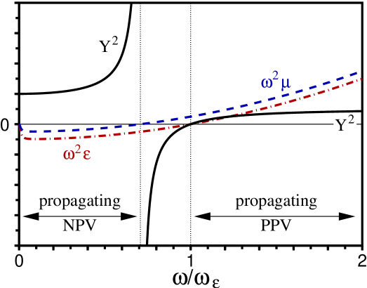
Examining the respective roles of the reference permittivity and permeability in eqns. (13) and (16), (17), we see that as far as dispersion and other linear effects are concerned, the two components simply add. In contrast, their effect on nonlinear terms is more dramatic: with the ratio scaling the nonlinear corrections to the magnetization into the electric field units of . This is because determines how much of a given directional field is electric field and how much magnetic field; large values of correspond to cases where the magnetic field is most prominent. Indeed, is just the reciprocal of the electromagnetic impedance of our chosen reference medium, and only if is real-valued do propagating fields exist, since otherwise the fields become evanescent.
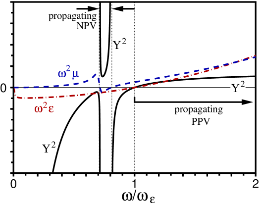
Figures 1 and 2 show how varies with frequency for two different metamaterial types, with the dispersions encoded on and and scaled by to moderate the low-frequency singularity of the Drude response. The extreme limits of large occur when , that is, usually just at an edge of a non-propagating band, where is about to change sign. In such a region, it would be better to revert to the fields, or to rescale the propagation equations into units of magnetic field (e.g., with some ).
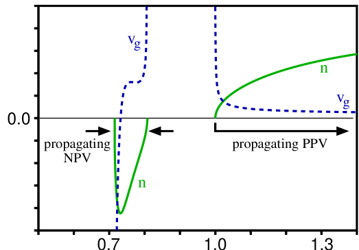
In previous work Scalora et al. (2005); Wen et al. (2007); D’Aguanno et al. (2008), a Drude type response for both and was assumed, where ; and this situation is shown on Fig. 1. However, although the dielectric response in metamaterials (e.g., a wire grid array Pendry-HSY-1996prl; Pendry-HRS-1998jpcm) often has this behaviour, the magnetic response of split ring resonators (SRRs) differs. SRR magnetization is best described by a pseudo-Lorentz model333Also known as the “F-model” Pendry-HRS-1999ieeemtt with , although sometimes a true Lorentz response is used instead, . Note the difference between the numerators in these latter two expressions: a frequency-dependent versus a constant material parameter . The pseudo-Lorentz model has an incorrect high-frequency behaviour, and so it is incompatible with the Kramers-Kronig relations that enforce causality. However, at low and medium frequency it is a better match to the physical response of SRRs, and so I use it for Figs. 2 and 3.
There are frequency ranges over which the linear material responses vary dramatically, and in particular on Fig. 3 (which uses the same model as Fig. 2) this is evident for both the refractive index and group velocity . If we aim to operate in such regions, this leads to two potential complications. First, if we have chosen reference parameters that do not match the linear material responses exactly, then the correction terms will become large, meaning that our wavelength-scale “slow evolution” approximation may come under threat. Second, even if our reference parameters do match the linear material responses exactly, our wavelength-scale will have become frequency dependent, and so again our “slow evolution” approximation may be threatened. In either case the solution is simple – we just need to revert to the bi-directional wave equations [i.e., eqns. (9) or (10)]. However, this does not necessarily mean that any backward evolving fields are generated (as explained in Kinsler et al. (2005), and following a different approach in Kinsler (2008)), so that in principle one could optimize the propagation by reinstating it only over those frequency ranges where it becomes necessary.
VII Conclusions
I have derived a uni-directional optical pulse propagation equation for media with both electric and magnetic responses, based on the directional fields approach Kinsler et al. (2005). This involved a re-expression of Maxwell’s equations, and required only a single approximation to reduce a one dimensional bi-directional model, to a uni-directional first-order wave equation. The simplicity of this approach makes it very convenient in waveguides, optical fibres, or other collinear situations. The important approximation is that the pulse evolves only slowly on the scale of a wavelength; and indeed this is a valid assumption in a wide variety of cases – note in particular that nonlinear effects have to be unrealizably strong to violate it Kinsler (2007b). The result has no intrinsic bandwidth restrictions, makes no demands on the pulse profile, and does not require a co-moving frame – unlike other common types of derivation Agrawal (2007); Brabec and Krausz (1997); Geissler et al. (1999); Kinsler and New (2003).
The resulting equations have the advantage that they are straightforward to write down, despite containing the complications of both electric and magnetic responses, and that a carrier-envelope representation or co-moving frames are easy to apply if desired, requiring no further approximation. In this, they match the clarity and flexibility of factorized second-order wave equations Ferrando et al. (2005); Genty et al. (2007); Kinsler (2008), but they can more easily incorporate the effects of magnetic material responses – albiet at the cost of being restricted to one dimensional propagation.
Acknowledgements.
I acknowledge financial support from the Engineering and Physical Sciences Research Council (EP/E031463/1).References
-
Pendry (2000)
J. B. Pendry,
Phys. Rev. Lett. 85, 3966 (2000),
doi:10.1103/PhysRevLett.85.3966. -
Tsakmakidis et al. (2007)
K. L. Tsakmakidis,
A. D. Boardman,
and O. Hess,
Nature 450, 397 (2007),
doi:10.1038/nature06285. -
Scalora et al. (2005)
M. Scalora,
M. S. Syrchin,
N. Akozbek,
E. Y. Poliakov,
G. D’Aguanno,
N. Mattiucci,
M. J. Bloemer,
and A. M.
Zheltikov,
Phys. Rev. Lett. 95, 013902 (2005),
doi:10.1103/PhysRevLett.95.013902. -
Wen et al. (2007)
S. Wen,
Y. Xiang,
X. Dai,
Z. Tang,
W. Su, and
D. Fan,
Phys. Rev. A 75, 033815 (2007),
doi:10.1103/PhysRevA.75.033815. -
D’Aguanno et al. (2008)
G. D’Aguanno,
N. Mattiucci,
and M. J.
Bloemer,
J. Opt. Soc. Am. B 25, 1236 (2008),
doi:10.1364/JOSAB.25.001236. -
Kinsler and New (2003)
P. Kinsler and
G. H. C. New,
Phys. Rev. A 67, 023813 (2003),
doi:10.1103/PhysRevA.67.023813,
arXiv:physics/0212016. -
Brabec and Krausz (1997)
T. Brabec and
F. Krausz,
Phys. Rev. Lett. 78, 3282 (1997),
doi:10.1103/PhysRevLett.78.3282. -
Geissler et al. (1999)
M. Geissler,
G. Tempea,
A. Scrinzi,
M. Schnürer,
F. Krausz, and
T. Brabec,
Phys. Rev. Lett. 83, 2930 (1999),
doi:10.1103/PhysRevLett.83.2930. -
Agrawal (2007)
G. P. Agrawal,
Nonlinear Fiber Optics
(Academic Press, Boston, 2007), 4th ed., ISBN 978-0-12-369516-1. - Kinsler (2002) P. Kinsler (2002), arXiv:physics/0212014.
-
Kinsler et al. (2005)
P. Kinsler,
S. B. P. Radnor,
and
G. H. C. New,
Phys. Rev. A 72, 063807 (2005),
doi:10.1103/PhysRevA.72.063807, arXiv:physics/0611215. -
Kinsler (2007a)
P. Kinsler
(2007a),
“Pulse propagation methods in nonlinear optics”,
arXiv:0707.0982. -
Kinsler et al. (2009)
P. Kinsler,
A. Favaro, and
M. W. McCall,
Eur. J. Phys. 30, 983 (2009),
doi:10.1088/0143-0807/30/5/007, arXiv:0908.1721. -
Kinsler (2007b)
P. Kinsler,
J. Opt. Soc. Am. B 24, 2363 (2007b),
doi:10.1364/JOSAB.24.002363, arXiv:0707.0986. -
Kinsler (2008)
P. Kinsler,
Phys. Rev. A 81, 013819 (2008),
doi:10.1103/PhysRevA.81.013819, arXiv:0810.5689. -
Fleck (1970)
J. A. Fleck,
Phys. Rev. B 1, 84 (1970),
doi:10.1103/PhysRevB.1.84. -
Scalora and Crenshaw (1994)
M. Scalora and
M. E. Crenshaw,
Opt. Commun. 108, 191 (1994),
doi:10.1016/0030-4018(94)90647-5. -
Kinsler and New (2004)
P. Kinsler and
G. H. C. New,
Phys. Rev. A 69, 013805 (2004),
doi:10.1103/PhysRevA.69.013805,
arXiv:physics/0411120. -
Kinsler and New (2005)
P. Kinsler and
G. H. C. New,
Phys. Rev. A 72, 033804 (2005),
doi:10.1103/PhysRevA.72.033804,
arXiv:physics/0606111. -
Kinsler et al. (2006)
P. Kinsler,
G. H. C. New,
and J. C. A.
Tyrrell
(2006), arXiv:physics/0611213. -
Boyd (2003)
R. W. Boyd,
Nonlinear Optics
(Academic Press, New York, 2003), 2nd ed., 1st ed. 1994. -
Gabor (1946)
D. Gabor,
J. Inst. Electr. Eng. (London) 93, 429 (1946). -
Laegsgaard (2007)
J. Laegsgaard,
Opt. Express 15, 16110 (2007),
doi:10.1364/OE.15.016110. -
Boardman et al. (2000)
A. D. Boardman,
K. Marinov,
D. I. Pushkarov,
and
A. Shivarova,
Optical and Quantum Electronics 32, 49 (2000),
doi:10.1023/A:1007045304098. -
Alfano and
Shapiro (1970a)
R. R. Alfano and
S. L. Shapiro,
Phys. Rev. Lett. 24, 584 (1970a), doi:10.1103/PhysRevLett.24.584. -
Alfano and
Shapiro (1970b)
R. R. Alfano and
S. L. Shapiro,
Phys. Rev. Lett. 24, 592 (1970b), doi:10.1103/PhysRevLett.24.592. -
Dudley et al. (2006)
J. M. Dudley,
G. Genty, and
S. Coen,
Rev. Mod. Phys. 78, 1135 (2006),
doi:10.1103/RevModPhys.78.1135. -
Solli et al. (2007)
D. R. Solli,
C. Ropers,
P. Koonath, and
B. Jalali,
Nature 450, 1054 (2007),
doi:10.1038/nature06402. -
Braun et al. (1995)
A. Braun,
G. Korn,
X. Liu,
D. Du,
J. Squier, and
G. Mourou,
Opt. Lett. 20, 7375 (1995),
doi:10.1364/OL.20.000073. -
Berge and Skupin (2009)
L. Berge and
S. Skupin,
Discrete and Continuous Dynamical Systems (DCDS-A) 23, 1099 (2009),
doi:10.3934/dcds.2009.23.1099. -
Various (1993)
Various, J. Opt. Soc. Am. B
10,
1656–1791 (1993),
”Special Issue on optical parametric oscillation and amplification”,
URL http://www.opticsinfobase.org/josab/issue.cfm?volume=10&issue%=9. -
Danielius et al. (1993)
R. Danielius,
A. Piskarskas,
A. Stabinis,
G. P. Banfi,
P. D. Trapani,
and R. Righini,
J. Opt. Soc. Am. B 10, 2222 (1993),
doi:10.1364/JOSAB.10.002222. -
Genty et al. (2007)
G. Genty,
P. Kinsler,
B. Kibler, and
J. M. Dudley,
Opt. Express 15, 5382 (2007),
doi:10.1364/OE.15.005382. -
Ferrando et al. (2005)
A. Ferrando,
M. Zacares,
P. F. de Cordoba,
D. Binosi, and
A. Montero,
Phys. Rev. E 71, 016601 (2005),
doi:10.1103/PhysRevE.71.016601. -
Kinsler (2006)
P. Kinsler,
(2006), arXiv:physics/0611216.
Appendix A Derivation of eqn. (1)
The derivation in this paper is simpler, more general, and defines using a better sign convention than those in Kinsler et al. (2005); Kinsler (2006). I start with the Maxwell curl equations, and transform into frequency space:
| (23) | ||||
| (24) |
I now rotate the equation by taking the cross product with u,
| (25) |
scale each part by and respectively, while insisting that these parameters do not depend on position. Thus,
| (26) |
and then take the sum and difference –
| (27) |
The vector fields are defined in eqn. (2), but that neglects the longitudinal part of H. Thus, for completeness, we also need to define (as in Kinsler et al. (2005); Kinsler (2006)). Their form means that I need to convert both the second term on the LHS of the sum-and-difference equation above, as well as the RHS. It is most important for the LHS to be simple, because this will define the type of propagation specified by the RHS. In the following I use the vector identity.
| (28) |
along with , so that
| (29) | ||||
| (30) | ||||
| (31) |
Continuing the derivation,
| (32) | ||||
| (33) | ||||
| (34) | ||||
| (35) |
I now rearrange eqn. (35) to give the final form, in which I substitute and to match eqn. (1). Thus
| (36) | ||||
| (37) |
and finally
| (38) | ||||
| (39) |
Note that for , where is some complicated but scalar dielectric response function, we have
| (40) | ||||
| (41) |
and for , where is some complicated but scalar magnetic response function, we have
| (42) | ||||
| (43) | ||||
| (44) | ||||
| (45) |
Finally, when generating eqn. (25), we lost the longitudinal part of (i.e. that parallel to u). This is
| (46) | ||||
| (47) | ||||
| (48) |
| (49) |
since , and
| (50) | ||||
| (51) |
Appendix B Correction terms
In this appendix I work through the details of how the polarization and magnetization terms scale with respect to one another. To simplify matters, I assume all corrections are scalar since when and are not field-polarization or orientation sensitive, the scalings remain the same, even if the specific field terms may vary (e.g. instead of ).
Consider the general unidirectional equation for (i.e. eqn. (10)), and replace the polarization and magnetization terms with dimensionless response parameters and multiplied by the appropriate field or . Then replace and with their representation in terms of , so that
| (52) | ||||
| (53) | ||||
| (54) | ||||
| (55) |
remembering that , and that , and .
Since we consider the electric-field-like field , the polarization corrections are trivial to write down; as for an -th order nonlinear term, . This means we need only concentrate on the magnetization correction. If is that for an -th order nonlinear term, then . Writing down only the term in square brackets from eqn. (55) gives us
| (56) | |||
| (57) |
Note that corrections for linear loss or gain are first-order processes (i.e. with ), where for loss we need , with ; Thus for loss the whole correction term will be proportional to , as would be expected.