A Unified Stability Analysis of Safety-Critical Control using Multiple Control Barrier Functions

Matheus F. Reis, José P. Carvalho and A. Pedro Aguiar The authors are with the Research Center for Systems and Technologies (SYSTEC-ARISE), Faculdade de Engenharia, Universidade do Porto, Rua Dr. Roberto Frias, s/n 4200-465, Porto, Portugal {matheus.reis, jpcarvalho, apra}@fe.up.pt

Abstract

Ensuring liveness and safety of autonomous and cyber-physical systems remains a fundamental challenge, particularly when multiple safety constraints are present. This letter advances the theoretical foundations of safety-filter Quadratic Programs (QP) and Control Lyapunov Function (CLF)-Control Barrier Function (CBF) controllers by establishing a unified analytical framework for studying their stability properties. We derive sufficient feasibility conditions for QPs with multiple CBFs and formally characterize the conditions leading to undesirable equilibrium points at possible intersecting safe set boundaries. Additionally, we introduce a stability criterion for equilibrium points, providing a systematic approach to identifying conditions under which they can be destabilized or eliminated. Our analysis extends prior theoretical results, deepening the understanding of the conditions of feasibility and stability of CBF-based safety filters and the CLF-CBF QP framework.

I INTRODUCTION

Due to recent technological advancements, cyber-physical and autonomous systems, including self-driving vehicles and robotics, are becoming increasingly prevalent in our lives. While these systems exhibit higher autonomy levels, the increase in agency also brings more unpredictable and catastrophic failures [2], making it ever more crucial to design controllers that are both performant and provably safe.

The performance of a controller can be associated with its liveness, defined as asymptotic stability towards a set of goal states. On the other hand, safety can be defined as the requirement of forward invariance of the system trajectories with respect to a specified safe set. Combining and guaranteeing the fulfillment of these two requirements is still an open problem. Common approaches are the safety filter architecture [3] and the CLF-CBF minimum-norm controller [1]. In the former, the liveness and safety requirements are decoupled through a performance (nominal) controller that seeks to ensure liveness, while a safety controller modifies the control law to guarantee safety at all times [11], making use of Control Barrier Functions (CBFs) [6] to model the safety requirements. In the latter, safety and liveness are directly combined within an unified control framework [1], using Control Lyapunov Functions (CLFs) and CBFs.

However, it is shown in [8] that due to the conflicting objectives of safety and liveness, the CLF-CBF QP framework can introduce undesirable stable equilibrium points on the safe set boundary. This means that while the framework can guarantee safety, it does not guarantee liveness as the system’s trajectories can get stuck at undesirable equilibrium points, resulting in deadlocks. Research has aimed to mitigate or avoid these deadlocks in both the CLF-CBF framework and CBF-based safety filters.

In [7], a method is proposed to solve the deadlock problem for the safety-filter considering multiple non-convex unsafe regions modeled by CBFs. Undesirable stable equilibria are avoided by using a nonlinear transformation that maps the system state into a new domain called the “ball world”, where all non-convex CBF boundaries are converted into moving $n$ -spheres and dynamically avoid the state trajectory. In [8], the authors propose a solution based on a rotating CLF, so that equilibrium points are removed in the case of a single convex unsafe set. The idea of modifying the CLF to avoid deadlocks is latter extended in [9], where the theory of linear matrix polynomials was used to compute a CLF that does not cause deadlocks, considering the class of linear systems and quadratic CLFs and CBFs. Finally, in [5], the authors address the deadlock problem by proposing a learning-based framework that adapts the CBF class $\mathcal{K}$ function online. Using a probabilistic ensemble neural network (PENN), the framework predicts safety and performance metrics, including deadlock time, which is then minimized to mitigate deadlocks.

This paper builds upon the work [9] and presents a generalized theoretical understanding for the conditions for the formation of undesirable boundary equilibrium points with the CBF-based safety filters and CLF-CBF frameworks for safety-critical control. Particularly:

•

Addresses the stability theory for the closed-loop system of affine nonlinear systems with both the safety-filter QP and CLF-CBF mininum-norm QP using a single, generalized QP framework for both safety-critical controllers.
•

Derives sufficient conditions for the feasibility of the safety-filter QP and CLF-CBF QP with multiple CBFs.
•

Introduces conditions for existence of undesirable equilibrium points that are valid both for the safety-filter QP and for the CLF-CBF QP, considering multiple, possibly overlapping CBF unsafe sets.
•

Derives a novel condition for the stability of boundary equilibrium points of this type with a clear geometric intuition.

II PRELIMINARIES

Notation: Given a matrix $A\in\mathbb{R}^{n\times m}$ or vector $v\in\mathbb{R}^{n}$ $[A]_{k}\in\mathbb{R}^{n}$ denotes its $k$ -th column and $[v]_{k}\in\mathbb{R}$ denotes its $k$ -th element, while $\text{diag}\{\alpha_{1},\,\cdots,\,\alpha_{r}\}$ is block matrix with the diagonal stacking of $r$ scalars or matrices $\alpha_{1},\,\cdots,\,\alpha_{r}$ . Matrix $I_{n}\in\mathbb{R}^{n\times n}$ is the $n\times n$ identity matrix. $L_{g}f$ is the Lie derivative of a function $f$ along a function $g:\mathbb{R}^{n}\rightarrow\mathbb{R}^{n\times m}$ , that is, $L_{g}f=\nabla f^{\mathsf{T}}g\in\mathbb{R}^{m}$ . The inner product between two vectors $u,v\in\mathbb{R}^{n}$ induced by a positive semidefinite matrix $X=X^{\mathsf{T}}\geq 0$ is given by $\langle u,v\rangle_{X}=u^{\mathsf{T}}X\,v$ . This inner product induces a norm $\lVert v\rVert_{X}^{2}=\langle v,v\rangle_{X}=v^{\mathsf{T}}X\,v$ over $\mathbb{R}^{n}$ . The standard inner product is then $\langle u,v\rangle=\langle u,v\rangle_{I_{n}}$ , with standard Euclidean norm $\lVert v\rVert^{2}=\lVert v\rVert_{I_{n}}^{2}$ . The orthogonal complement of a subspace $\mathcal{W}$ is denoted by $\mathcal{W}^{\perp}$ , with orthogonality dependent on an inner product $\langle\cdot,\cdot\rangle_{X}$ .

II-A Control Lyapunov (CLFs) and Barrier Functions (CBFs)

Consider the nonlinear control affine system

\displaystyle\dot{x}=f(x)+g(x)u

(1)

where $x\in\mathbb{R}^{n}$ , $u\in\mathbb{R}^{m}$ are the system state and control input, respectively, and $f:\mathbb{R}^{n}\rightarrow\mathbb{R}^{n}$ , $g:\mathbb{R}^{n}\rightarrow\mathbb{R}^{n\times m}$ are locally Lipschitz.

Definition II.1 (CLFs).

A positive definite function $V$ is a control Lyapunov function (CLF) for system (1) if it satisfies:

\displaystyle\inf_{u\in\mathbb{R}^{m}}\left[L_{f}V(x)+L_{g}Vu\right]\leq-\gamma(V(x))

where $\gamma:\mathbb{R}_{\geq 0}\rightarrow\mathbb{R}_{\geq 0}$ is a class $\mathcal{K}$ function [4].

Definition II.1 implies that there exists a set of stabilizing controls that makes the CLF strictly decreasing everywhere outside its global minimum $x_{0}\in\mathbb{R}^{n}$ , given by $\mathbb{K}_{V}(x)=\{u\!\in\!\mathbb{R}^{m}:L_{f}V+L_{g}Vu\leq-\gamma(V)\}$ .

Definition II.2 (Safety).

The trajectories of a given system are safe with respect to a set $\mathcal{C}$ if $\mathcal{C}$ is forward invariant, meaning that for every $x(0)\in\mathcal{C}$ , $x(t)\in\mathcal{C}$ for all $t>0$ .

Consider $N$ subsets $\mathcal{C}_{1},\dots,\mathcal{C}_{N}\subset\mathbb{R}^{n}$ defined by the superlevel set of $N$ continuously differentiable functions $h_{i}:\mathbb{R}^{n}\rightarrow\mathbb{R}$ , $i=1,2,\ldots,N$ The corresponding $i$ -th boundary is given by $\partial\mathcal{C}_{i}=\{x\in\mathbb{R}^{n}:h_{i}(x)=0\}$ .

Definition II.3 (CBFs).

Let $\mathcal{C}_{i}=\{x\in\mathbb{R}^{n}:h_{i}(x)\geq 0\}$ . Then $h_{i}(x)$ is a (zeroing) Control Barrier Function (CBF) for (1) if there exists a locally Lipschitz extended class $\mathcal{K}_{\infty}$ function [4] $\alpha_{i}:\mathbb{R}\rightarrow\mathbb{R}$ such that

\displaystyle\sup_{u\in\mathbb{R}^{m}}\left[L_{f}h_{i}(x)+\langle L_{g}h_{i}(x),u\rangle\right]\geq-\alpha_{i}(h_{i}(x))

This definition means that there exists a set of safe controls allowing the $i$ -th CBF to decrease on in the interior of its safe set $\text{int}(\mathcal{C}_{i})$ , but not on its boundary $\partial\mathcal{C}_{i}$ , given by $\mathbb{K}_{h_{i}}(x)\!=\!\{u\in\mathbb{R}^{m}\!:\!L_{f}h_{i}\!+\!L_{g}h_{i}u\!+\!\alpha_{i}(h_{i})\geq 0\}$ . The composite safe set associated to all the $N$ CBFs is simply $\mathcal{C}=\bigcap^{N}_{i=1}\mathcal{C}_{i}$ and the set of controls rendering $\mathcal{C}$ forward invariant is the intersection $\mathbb{K}_{h}(x)=\bigcap^{N}_{i=1}\mathbb{K}_{h_{i}}(x)$ .

II-B QP-Based Safety-Critical Controllers

Consider the closed-loop system for (1)

\displaystyle\dot{x}=f_{cl}(x):=f(x)+g(x)u^{\star}(x)

(2)

with a state-feedback control law $u^{\star}(x)$ . A common approach for safety-critical control is the safety-filter algorithm, which minimally modifies a given stabilizing state-feedback control law $u_{nom}(x)$ to achieve safety. The safety-filter effectively generates the “closest” safe control $u^{\star}(x)\in\mathbb{K}_{h}(x)$ to the stabilizing control $u_{nom}(x)$ .

An alternative approach that also makes use of QPs is the minimum-norm CLF-CBF QP by [1]:

$\displaystyle u^{\star}(x),\delta^{\star}(x)$	$\displaystyle=\operatorname*{argmin}_{(u,\delta)}\frac{1}{2}(\Delta u)^{\mathsf{T}}H(x)(\Delta u)+\frac{1}{2}p\delta^{2}$	(3)
$\displaystyle s.t.\,$	$\displaystyle L_{f}V+\langle L_{g}V(x),u\rangle\leq-\gamma(V)+\delta$	(CLF)
	$\displaystyle L_{f}h_{i}+\langle L_{g}h_{i}(x),u\rangle\geq-\alpha_{i}(h_{i})$	(CBFs)

$i\in\{1,\cdots,N\}$ , $H:\mathbb{R}^{n}\rightarrow\mathbb{R}^{n\times n}$ being a symmetric positive definite matrix function of the state, $p>0$ and (for now) $\Delta u=u$ . The relaxation variable $\delta$ in the CLF constraint softens the stabilization objective, aiming to maintain the feasibility of the QP. If feasible, the feedback controller (3) with $\Delta u=u$ generates a minimum-norm stabilizing and safe control, guaranteeing local stability of the origin and safety of the closed-loop system trajectories with respect to the composite safe set $\mathcal{C}$ .

As pointed out by the works [8, 9, 10], neither the safety-filter nor the CLF-CBF QP (3) (with $\Delta u=u$ ) can guarantee global stabilization of trajectories towards the origin for the closed-loop system (2), meaning that trajectories could converge towards undesirable equilibrium points. Here, our objective is to study the solutions, existence conditions and stability of equilibrium points of the closed-loop system formed by a generalized QP controller given by (3) with $\Delta u=u-u_{nom}(x)$ , where $u_{nom}$ is the stabilizing control law from the safety-filter QP. The structure of controller (3) with $\Delta u=u-u_{nom}(x)$ allows for the generalization of the safety-filter and the CLF-CBF QPs into a single framework:

1.

with $H(x)=I_{m}$ and $V=0$ (without CLF), we recover the usual safety-filter QP. In this case, the optimal solution for the slack variable is always $\delta^{\star}=0$ .
2.

with $u_{nom}(x)=0$ , we recover the usual CLF-CBF QP.

If feasible, the solution of the generalized QP (3) is guaranteed $u^{\star}(x)\in\mathbb{K}_{h}(x)$ , and possibly close to the stabilizing set $\mathbb{K}_{V}(x)$ . However, due to the slack variable, it is not possible to strictly guarantee that $u^{\star}(x)\in\mathbb{K}_{V}(x)\cap\mathbb{K}_{h}(x)\,\,\forall x\in\mathbb{R}^{n}$ . That means that safety with respect to $\mathcal{C}$ is achieved, but stabilization is (possibly) hampered.

Assumption II.1.

The initial state $x(0)\in\mathbb{R}^{n}$ and the origin $0\in\mathbb{R}^{n}$ are contained in the safe set $\mathcal{C}$ , that is, $h_{i}(x(0))\geq 0$ and $h_{i}(0)\geq 0$ for all $i\in\{1,\cdots,N\}$ .

Theorem 1.

Under Assump. II.1, consider the following assumptions:
(i) There is only one CBF ( $N=1$ ).
(ii) System (1) is driftless: $f(x)=0\,\,\,\forall x\in\mathbb{R}^{n}$ .
(iii) Considering any number of CBFs ( $N>1$ ),

	$\displaystyle b_{2}(x)$	$\displaystyle\in\operatorname{Im}{U^{\mathsf{T}}\mathcal{P}_{V}GU}$		(4)
	$\displaystyle b_{2}(x)$	$\displaystyle=U^{\mathsf{T}}\left(c^{-1}\gamma(V)G\nabla V-\mathcal{P}_{V}f_{nom}\right)-\bar{\alpha}$

where $c\!=\!p^{-1}\!+\!\lVert\nabla V\rVert_{G}^{2}>0$ , $G(x)\!=\!g(x)H(x)^{-1}g(x)^{\mathsf{T}}$ , $f_{nom}(x)\!=\!f(x)\!+\!g(x)u_{nom}(x)$ , $\mathcal{P}_{V}=I-c^{-1}G\nabla V\nabla V^{\mathsf{T}}$ , $\bar{\alpha}\!=\!\begin{bmatrix}\,\alpha_{1}(h_{1})\!\!\!&\!\!\!\cdots\!\!\!&\!\!\!\alpha_{N}(h_{N})\,\end{bmatrix}^{\mathsf{T}}$ and $U(x)\!=\!\begin{bmatrix}\,\nabla h_{1}\!\!\!&\!\!\!\cdots\!\!\!&\!\!\!\nabla h_{N}\,\end{bmatrix}$ .
Then, QP (3) is feasible under Assumptions (i) or (ii) or (iii).

Proof.

The proofs of (i) and (ii) can be found in [1] and [9], respectively. To establish the proof of (iii), we begin by formulating the Lagrangian associated with the QP (3)

$\displaystyle\mathcal{L}(u,\delta,\bar{\lambda})\!$	$\displaystyle=\!\frac{1}{2}\left(\lVert\Delta u\rVert_{H}^{2}\!+\!p\delta^{2}\right)$	(5)
	$\displaystyle\!+\lambda_{0}(L_{f}V\!+\!\langle L_{g}V,u\rangle\!+\!\gamma(V)\!-\!\delta)$
	$\displaystyle\!-\sum^{N}_{i=1}\lambda_{i}(L_{f}h_{i}\!+\!\langle L_{g}h_{i},u\rangle\!+\!\alpha_{i}(h_{i}))$

where $\lambda_{i}\geq 0$ and $\lambda\!=\!\begin{bmatrix}\,\lambda_{1}\!\!\!&\!\!\!\cdots\!\!\!&\!\!\!\lambda_{N}\,\end{bmatrix}^{\mathsf{T}}\in\mathbb{R}^{N}_{\geq 0}$ , $\bar{\lambda}\!=\!\begin{bmatrix}\,\lambda_{0}\!\!&\!\!\lambda^{\mathsf{T}}\,\end{bmatrix}^{\mathsf{T}}\in\mathbb{R}^{N+1}_{\geq 0}$ are vectors of KKT multipliers associated to the optimization problem. Using matrix $U$ , the stationarity KKT conditions give the following solutions for the QP:

	$\displaystyle u^{\star}(x)$	$\displaystyle=u_{nom}+H^{-1}g^{\mathsf{T}}\left(-\lambda_{0}\nabla V+U\lambda\right)$		(6)
	$\displaystyle\delta^{\star}(x)$	$\displaystyle=p^{-1}\lambda_{0}$		(7)

The dual function $g(\bar{\lambda})=\min_{(u,\delta)}\mathcal{L}(u,\delta,\bar{\lambda})$ associated to the QP can be obtained by substituting (6) into (5), yielding the following dual QP:

	$\displaystyle\max_{\bar{\lambda}\in\mathbb{R}^{N}_{\geq 0}}$	$\displaystyle-\frac{1}{2}\bar{\lambda}^{\mathsf{T}}A(x)\bar{\lambda}+\bar{\lambda}^{\mathsf{T}}b(x)$		(8)
	$\displaystyle A(x)$	$\displaystyle=\begin{bmatrix}c\!\!&\!\!-\nabla V^{\mathsf{T}}GU\\ -U^{\mathsf{T}}G\nabla V\!\!&\!\!U^{\mathsf{T}}GU\end{bmatrix}\,,\,\,b(x)=\begin{bmatrix}F_{V}\\ -F_{h}\end{bmatrix}$

with $F_{V}=L_{f_{nom}}V+\gamma(V)$ , $F_{h}=U^{\mathsf{T}}f_{nom}+\bar{\alpha}$ . Notice that the dual cost in (8) is bounded from above if and only if $b(x)\in\operatorname{Im}{A(x)}$ . In that case, the primal QP (3) is feasible. Applying Gauss elimination to the augmented matrix $\begin{bmatrix}\,A(x)\!\!&\!\!\!\!|\!\!\!\!&\!\!b(x)\,\end{bmatrix}$ yields

\displaystyle\begin{bmatrix}1\!\!&\!\!-c^{-1}\nabla V^{\mathsf{T}}GU\!\!\!&|&\!\!\!c^{-1}F_{V}\\ 0\!\!&\!\!U^{\mathsf{T}}\mathcal{P}_{V}GU\!\!\!&|&\!\!\!b_{2}(x)\end{bmatrix}

(9)

Then, from (9), the condition $b_{2}(x)\in\operatorname{Im}{U^{\mathsf{T}}\mathcal{P}_{V}GU}$ as stated in (4) is equivalent to $b(x)\in\operatorname{Im}{A(x)}$ , meaning that the primal QP is feasible under this condition. ∎

Theorem 1(iii) provides a sufficient condition for the feasibility of QP (3): when (4) holds, the corresponding dual QP cost is bounded, which means (3) is feasible. Feasibility condition (4) is of particular importance when assumptions (i) and (ii) fail, giving a sufficient condition for the feasibility of QP (3) in the case when multiple safety objectives are simultaneously required.

III Closed-loop System Analysis

III-A Existence of Equilibrium Points

In this section, we extend a result from [8], regarding the existence of equilibrium points in the safety-filter QP or in the CLF-CBF QP when multiple CBF constraints are present. The results are conditioned to the feasibility of the QP (3): that is, it is assumed that at least one of the conditions of Theorem 1 holds.

Definition III.1 (Equilibrium Manifold).

Let the set $\mathcal{A}=\{a_{1},\cdots,a_{r}\}\subset 2^{\{1,\cdots,N\}}$ be a collection of $1\leq r\leq N$ CBF indexes corresponding to $r$ CBFs $\{h_{a_{1}},\cdots,h_{a_{r}}\}$ . Define the vector field $f_{\mathcal{A}}:\mathbb{R}^{n}\times\mathbb{R}^{r}_{\geq 0}\rightarrow\mathbb{R}^{n}$ :

	$\displaystyle f_{\mathcal{A}}(x,\lambda)$	$\displaystyle=f_{nom}-p\gamma(V)G\nabla V+GU_{\!\mathcal{A}}\lambda$		(10)
	$\displaystyle U_{\!\mathcal{A}}$	$\displaystyle=\begin{bmatrix}\,\nabla h_{a_{1}}\!\!&\!\!\cdots\!\!&\!\!\nabla h_{a_{r}}\,\end{bmatrix}\in\mathbb{R}^{n\times r}$		(11)

As will be demonstrated in the next sections, (10) and its Jacobian with respect to $x$ will be of central importance to characterize the existence and stability conditions for the equilibrium points of the closed-loop system.

Theorem 2 (Existence of Equilibrium Points).

Let (2) be the closed-loop system formed by the nonlinear system (1) with controller (3). Let the set $\mathcal{A}$ as defined in Definition III.1 representing the indexes of $r$ overlapping CBF boundaries $\partial\mathcal{C}_{\mathcal{A}}=\bigcap^{r}_{i=1}\partial\mathcal{C}_{a_{i}}\neq\emptyset$ . The equilibrium points of (2) come in two distinct types:

	$\displaystyle\mathcal{E}_{\partial\mathcal{C}_{\mathcal{A}}}\!$	$\displaystyle=\!\partial\mathcal{C}_{\mathcal{A}}\!\cap\!\{x\in\mathbb{R}^{n}\,\|\,\exists\lambda\!\in\!\mathbb{R}^{r}_{\geq 0}\text{ s.t. }f_{\mathcal{A}}(x,\lambda)\!=\!0\}$		(12)
	$\displaystyle\mathcal{E}_{int(\mathcal{C})}\!$	$\displaystyle=\!int(\mathcal{C})\!\cap\!\{x\in\mathbb{R}^{n}\,\|\,f_{nom}\!=\!p\gamma(V)G\nabla V\}$		(13)

where $\mathcal{E}_{\partial\mathcal{C}_{\mathcal{A}}}$ is the set of boundary equilibrium points occurring in $\partial\mathcal{C}_{\mathcal{A}}$ and $\mathcal{E}_{int(\mathcal{C})}$ is the set of interior equilibrium points. Furthermore, defining the region of the state space where only the $a_{1},\cdots,a_{r}$ CBF constraints are simultaneously active as $\mathcal{S}_{\mathcal{A}}\subset\mathbb{R}^{n}$ , we have $\mathcal{E}_{\partial\mathcal{C}_{\mathcal{A}}}\subset\mathcal{S}_{\mathcal{A}}$ .

Proof.

Substituting (6) in (2) and using the definition of $G(x)$ yields the following closed-loop dynamics:

\displaystyle f_{cl}(x)=f_{nom}(x)+G(x)\left(-\lambda_{0}\nabla V+U\lambda\right)

(14)

At an equilibrium point $x_{e}\in\mathcal{E}$ , $f_{cl}(x_{e})=0$ . Applying this condition to (2) yields

\displaystyle f_{nom}(x_{e})=G(x_{e})\left(\lambda_{0}\nabla V(x_{e})-U(x_{e})\lambda\right)

(15)

Case 1. Consider the region of the state space where the CLF constraint is inactive: $L_{f_{cl}}V+\gamma(V)-\delta^{\star}<0$ . Following the exact same steps of Case 1 of Theorem 2 on [9], we conclude that no equilibrium points can occur at this region. Case 2. Consider the region where CLF constraint is active: $L_{f_{cl}}V+\gamma(V)=\delta^{\star}$ . In the case of the safety-filter, since $V=0$ , the CLF constraint becomes simply $0\leq\delta$ and since the optimal solution for the relaxation variable is always $\delta^{\star}=0$ , the CLF constraint is always active. At an equilibrium point $x_{e}\in\mathcal{E}$ , $L_{f_{cl}}V(x_{e})=0$ . Therefore, using (7), $\gamma(V(x_{e}))=\delta^{\star}(x_{e})=p^{-1}\lambda_{0}$ . Then, at any equilibrium point $x_{e}\in\mathcal{E}$ , the multiplier associated to the CLF constraint is $\lambda_{0}(x_{e})=p\gamma(V(x_{e}))\geq 0$ . Therefore, equation (15) yields

\displaystyle f_{nom}(x_{e})\!=\!G(x_{e})\left(p\gamma(V(x_{e}))\nabla V(x_{e})-U(x_{e})\lambda\right)

(16)

For the safety-filter, $V=0$ and $\nabla V=0$ are valid in (16). For the next cases, the CLF constraint is assumed to be active.
Case 3. Consider the region where exactly $r\leq N$ CBF constraints are simultaneously active. Their corresponding indexes are denoted by the set $\mathcal{A}=\{a_{1},\cdots,a_{r}\}$ as defined previously. Therefore, $L_{f_{cl}}h_{i}+\alpha_{i}(h_{i})=0$ , for $i\in\mathcal{A}$ . At an equilibrium point $x_{e}$ occurring in this region, $L_{f_{cl}}h_{i}(x_{e})=0$ , implying that $h_{a_{1}}(x_{e})=\cdots=h_{a_{r}}(x_{e})=0$ . Therefore, $x_{e}$ must lie at the boundary intersection associated to the $r$ active CBFs, that is, $x_{e}\in\partial\mathcal{C}_{\mathcal{A}}$ . The conclusion is that boundary equilibrium points at $\partial\mathcal{C}_{\mathcal{A}}$ can only occur at $\mathcal{S}_{\mathcal{A}}$ , that is, the region where only the CBF constraints corresponding to $h_{a_{1}},\cdots,h_{a_{r}}$ are simultaneously active. Since in this case the remaining CBF constraints are all inactive, $\lambda_{i}=0\,\,\forall i\notin\mathcal{A}$ , and (16) reduces to

\displaystyle f_{nom}(x_{e})=G(x_{e})\left(p\gamma(V)\nabla V(x_{e})-U_{\mathcal{A}}(x_{e})\lambda_{a}\right)

(17)

where $U_{\mathcal{A}}$ is given by (11) and $\lambda_{a}\in\mathbb{R}^{r}_{\geq 0}$ is a vector of appropriate size with the non-negative corresponding KKT multipliers associated to the active CBF constraints. Notice that (17) is equivalent to $f_{\mathcal{A}}(x,\lambda_{a})=0$ as defined in (10). Thus, in this case, the equilibrium point is at the boundary intersection $\partial\mathcal{C}_{\mathcal{A}}$ and satisfies $f_{\mathcal{A}}(x_{e},\lambda_{a})=0$ for some $\lambda_{a}\in\mathbb{R}^{r}_{\geq 0}$ , demonstrating (12).
Case 4. Consider the region where all CBF constraints are inactive: $L_{f_{cl}}h_{i}+\alpha_{i}(h_{i})>0$ , $i=1,\cdots,N$ . Following the same steps of Case 4 of Theorem 2 on [9], we conclude that equilibrium points occurring in this region must lie in the interior of the safe set, that is, $x_{e}\in int(\mathcal{C})$ . Additionally, (16) must be satisfied with $\lambda=0$ , which means that $f(x_{e})=p\gamma(V(x_{e}))G(x_{e})\nabla V(x_{e})$ . This demonstrates (13). ∎

The work [10] has proposed a system transformation that removes certain types of interior equilibrium points from the closed-loop system with the CLF-CBF QP controller. We conjecture that a similar transformation could be performed in the case of the safety-filter. Thereby, in the remaining of the paper, we focus on the stability properties for boundary equilibrium points.

III-B Stability of Boundary Equilibrium Points

Lemma 1 (Closed-Loop Jacobian).

Let (2) be the closed-loop system formed by the nonlinear system (1) with controller (3), and let $\mathcal{A}$ from Definition III.1 represent the indexes of $1\leq r\leq n$ active CBF constraints. For a boundary equilibrium point $x_{e}\in\mathcal{E}_{\partial\mathcal{C}_{\mathcal{A}}}$ with full rank and $U_{\mathcal{A}}^{\mathsf{T}}(x_{e})g(x_{e})\neq 0$ , the Jacobian matrix $J_{cl}(x_{e})\in\mathbb{R}^{n\times n}$ of the closed-loop system (2) computed at $x_{e}$ is given by

	$\displaystyle J_{f_{cl}}(x_{e})\!$	$\displaystyle=\!\mathcal{P}_{U_{\mathcal{A}}}\!\left(\mathcal{P}_{V}J_{\mathcal{A}}(x_{e},\bar{\lambda}_{e})\!-\!c^{-1}\gamma^{\prime}(V)G\nabla V\nabla V^{\mathsf{T}}\right)$
		$\displaystyle\qquad\qquad\qquad-\mathcal{P}_{V}GU_{\mathcal{A}}S_{A}^{-1}\Lambda^{\prime}U_{\mathcal{A}}^{\mathsf{T}}$		(18)

where $\bar{\lambda}_{e}=\begin{bmatrix}\,p\gamma(V(x_{e}))&\lambda_{e}^{\mathsf{T}}\,\end{bmatrix}^{\mathsf{T}}$ , and $\lambda_{e}\in\mathbb{R}^{r}_{\geq 0}$ is the vector with the $r$ corresponding KKT multipliers at $x_{e}$ for the $r$ active CBF constraints, $\mathcal{P}_{U_{\mathcal{A}}}\!=\!I_{n}\!-\!\mathcal{P}_{V}GU_{\mathcal{A}}\,S_{A}^{-1}U^{\mathsf{T}}_{\mathcal{A}}$ with $S_{A}\!\!=\!U^{\mathsf{T}}_{\mathcal{A}}\mathcal{P}_{V}GU_{\mathcal{A}}$ , $\Lambda^{\prime}\!\!=\!\text{diag}\{\alpha^{\prime}_{a_{1}}\!(h_{a_{1}}),\!\cdots\!,\alpha^{\prime}_{a_{r}}\!(h_{a_{r}})\}\!>\!0$ and

\displaystyle J_{\mathcal{A}}(x,\bar{\lambda}_{a})\!

\displaystyle=\!\frac{\partial f_{nom}}{\partial x}\!-\!\lambda_{0}\frac{\partial(G\nabla V)}{\partial x}\!+\!\sum_{i\in\mathcal{A}}\frac{\partial(G\nabla h_{i})}{\partial x}\lambda_{i}

(19)

with $\bar{\lambda}_{a}=\begin{bmatrix}\,\lambda_{0}&\lambda_{a}^{\mathsf{T}}\,\end{bmatrix}^{\mathsf{T}}$ .

Remark III.1.

The Jacobian $J_{\mathcal{A}}$ as defined in (19) is not the same as $J_{f_{\mathcal{A}}}$ , the Jacobian of $f_{\mathcal{A}}$ in (10): they differ precisely by a factor of $p\gamma^{\prime}(V)\nabla V\nabla V^{\mathsf{T}}$ .

Proof.

This demonstration is a direct continuation of Case 3 from the proof of Theorem 2. Using the complementary slackness conditions, $\dot{V}+\langle L_{g}V,u^{\star}\rangle=\delta^{\star}$ , $\dot{h}_{i}+\langle L_{g}h_{i},u^{\star}\rangle=0\,\,\forall i\in\mathcal{A}$ . Substituting (6)-(7) these expressions and using the fact that $\lambda_{i}=0$ for all $i\notin\mathcal{A}$ yields the following system:

\displaystyle\underbrace{\begin{bmatrix}c\!&\!-\nabla V^{\mathsf{T}}GU_{\mathcal{A}}\\ -U_{\mathcal{A}}^{\mathsf{T}}G\nabla V\!&\!U_{\mathcal{A}}^{\mathsf{T}}GU_{\mathcal{A}}\end{bmatrix}}_{A_{a}(x)}\underbrace{\begin{bmatrix}\lambda_{0}\\ \lambda_{a}\end{bmatrix}}_{\bar{\lambda}_{a}}\!=\!\underbrace{\begin{bmatrix}F_{V}\\ -F_{h_{a}}\end{bmatrix}}_{b_{a}(x)}

(20)

where $\lambda_{a}\in\mathbb{R}^{r}_{\geq 0}$ , $F_{h_{a}}\!=U_{\mathcal{A}}^{\mathsf{T}}\,f_{nom}+\bar{\alpha}_{a}\in\mathbb{R}^{r}$ and $\bar{\alpha}_{a}\!=\!\begin{bmatrix}\,\alpha_{a_{1}}(h_{a_{1}})\!\!&\!\!\cdots\!\!&\!\!\alpha_{a_{r}}(h_{a_{r}})\,\end{bmatrix}^{\mathsf{T}}$ . Here, $A_{a}(x)\in\mathbb{R}^{(r+1)\times(r+1)}$ and $b_{a}(x)\in\mathbb{R}^{r+1}$ are essentially reduced versions of matrices $A(x)$ and $b(x)$ from (8), with fewer rows and columns (since not all constraints are active). In particular, the set $\mathcal{S}_{\mathcal{A}}$ where the CLF and only the CBF constraints from $\mathcal{A}$ are active is given by

\displaystyle\mathcal{S}_{\mathcal{A}}=\{x\in\mathbb{R}^{n}\,|\,

\displaystyle f_{cl}(x)\!=\!f_{nom}\!-\!\lambda_{0}G\nabla V\!+\!GU_{\mathcal{A}}\lambda_{a}\}

(21)

where $\lambda_{0},\lambda_{a}$ are the positive solutions of (20). Using the known formula for inversion of block matrices, since $c>0$ , $A_{a}(x)$ is invertible if its Schur complement $S_{A}=U^{\mathsf{T}}_{\mathcal{A}}\mathcal{P}_{V}GU_{\mathcal{A}}\in\mathbb{R}^{r\times r}$ is invertible. Since $\mathcal{P}_{V}(x)>0\,\forall x$ , $S_{A}^{-1}$ exists if $U_{\mathcal{A}}$ has full column rank and if $U^{\mathsf{T}}_{\mathcal{A}}(x)g(x)\neq 0$ . Under these assumptions, a formula for $A_{a}^{-1}(x)$ is

\displaystyle A_{a}^{-1}(x)\!=\!\!\begin{bmatrix}c^{-1}\!\!&\!\!0\\ 0\!\!&\!\!0\end{bmatrix}\!+\!\frac{1}{c^{2}}\!\!\begin{bmatrix}\nabla V^{\mathsf{T}}GU_{\mathcal{A}}\\ c\,I_{r}\end{bmatrix}\!S_{A}^{-1}\!\!\begin{bmatrix}\nabla V^{\mathsf{T}}GU_{\mathcal{A}}\\ c\,I_{r}\end{bmatrix}^{\mathsf{T}}\!\!\!

(22)

where the dimensions of vectors and matrices are conformable for matrix addition and multiplication. Then, the KKT multipliers $\lambda_{0}$ , $\lambda_{a}$ can be found by solving (20).

Taking the derivative of (20) with respect to the $k$ -th state component $x_{k}$ and solving for $\partial_{k}\bar{\lambda}_{a}$ yields

\displaystyle\partial_{k}\bar{\lambda}_{a}(x)

\displaystyle=A_{a}^{-1}\left(\partial_{k}b_{a}-\partial_{k}A_{a}\bar{\lambda}_{a}\right)

(23)

Defining $\bar{U}=\begin{bmatrix}\,-\nabla V\!\!&\!\!U_{\mathcal{A}}\,\end{bmatrix}\in\mathbb{R}^{n\times(r+1)}$ , the partial derivatives of $A_{a}(x)$ and $b_{a}(x)$ are:

	$\displaystyle\partial_{k}A_{a}(x)\!$	$\displaystyle=\!\partial_{k}(\bar{U}^{\mathsf{T}}G\bar{U})$		(24)
	$\displaystyle\partial_{k}b_{a}(x)\!$	$\displaystyle=\!-\partial_{k}(\bar{U}^{\mathsf{T}}f_{nom})\!-\!\bar{\Lambda}^{\prime}[\bar{U}^{\mathsf{T}}]_{k}$		(25)

where $\bar{\Lambda}^{\prime}=\text{diag}\{\gamma^{\prime}(V),\alpha^{\prime}_{a_{1}}(h_{a_{1}}),\,\cdots,\,\alpha^{\prime}_{a_{r}}(h_{a_{r}})\}$ . From (19), notice that $[J_{\mathcal{A}}]_{k}=\partial_{k}f_{nom}+\partial_{k}(G\bar{U})\bar{\lambda}_{a}$ . Using this fact, combining equations (24)-(25) to compute the term $\partial_{k}b_{a}-\partial_{k}A_{a}\bar{\lambda}_{a}$ in (23), left multiplying it by $A_{a}^{-1}$ and using the fact that $f_{cl}(x)=f_{nom}+G\bar{U}\bar{\lambda}_{a}$ yields

\displaystyle\partial_{k}\bar{\lambda}_{a}(x)\!

\displaystyle=\!-A_{a}^{-1}\!\left(\bar{U}^{\mathsf{T}}[J_{\mathcal{A}}]_{k}\!+\!\bar{\Lambda}^{\prime}[\bar{U}^{\mathsf{T}}]_{k}\!+\!(\partial_{k}\bar{U})^{\mathsf{T}}f_{cl}\right)

(26)

where the fact that $[J_{\mathcal{A}}]_{k}=\partial_{k}(f_{nom}+G\bar{U}\bar{\lambda}_{a})$ was used. Then, taking the derivative of the closed-loop system dynamics (2) with $\lambda_{i}=0\,\,\forall i\notin\mathcal{A}$ yields

\displaystyle\partial_{k}f_{cl}(x)=[J_{\mathcal{A}}]_{k}+G\bar{U}\partial_{k}\bar{\lambda}_{a}

(27)

which by using the expression for $\partial_{k}\bar{\lambda}_{a}$ in (26) yields an expression for the $k$ -th column of the closed-loop Jacobian matrix $J_{f_{cl}}(x)$ at $\mathcal{S}_{\mathcal{A}}$ . Consider an equilibrium point $x_{e}\in\mathcal{E}_{\partial\mathcal{C}_{\mathcal{A}}}$ . Since $f_{cl}(x_{e})=0$ by definition, the last term on the right-hand side of (23) vanishes. Then, substituting $\partial_{k}\bar{\lambda}_{a}(x_{e})$ in (27) and using the fact that $\lambda_{0}(x_{e})=p\gamma(V(x_{e}))$ yields

	$\displaystyle\partial_{k}f_{cl}(x_{e})$	$\displaystyle=(I\!-\!G\bar{U}A_{a}^{-1}\bar{U}^{\mathsf{T}})[J_{\mathcal{A}}(x_{e},\bar{\lambda}_{e})]_{k}$		(28)
		$\displaystyle\qquad\qquad\qquad-G\bar{U}A_{a}^{-1}\bar{\Lambda}^{\prime}[\bar{U}^{\mathsf{T}}]_{k}$

On the assumptions of the theorem, namely a full rank $U_{\mathcal{A}}(x_{e})$ and $U^{\mathsf{T}}_{\mathcal{A}}(x_{e})g(x_{e})\neq 0$ , equation (22) can be used to simplify the following expressions at (28):

$\displaystyle(I-G\bar{U}A_{a}^{-1}\bar{U}^{\mathsf{T}})$	$\displaystyle=\mathcal{P}_{U_{\mathcal{A}}}\mathcal{P}_{V}$	(29)
$\displaystyle G\bar{U}A_{a}^{-1}\bar{\Lambda}^{\prime}[\bar{U}^{\mathsf{T}}]_{k}$	$\displaystyle=c^{-1}\gamma^{\prime}(V)\mathcal{P}_{U_{\mathcal{A}}}G\nabla V[\nabla V]_{k}$
	$\displaystyle+\mathcal{P}_{V}GU_{\mathcal{A}}S_{A}^{-1}\Lambda^{\prime}[U_{\mathcal{A}}^{\mathsf{T}}]_{k}$	(30)

Substituting (29)-(30) in (28) yields

	$\displaystyle\partial_{k}f_{cl}(x_{e})\!$	$\displaystyle=\!\mathcal{P}_{U_{\mathcal{A}}}\!\left(\mathcal{P}_{V}J_{\mathcal{A}}(x_{e},\bar{\lambda}_{e})\!-\!c^{-1}\gamma^{\prime}(V)G\nabla V[\nabla V]_{k}\right)$
		$\displaystyle\qquad\qquad\qquad-\mathcal{P}_{V}GU_{\mathcal{A}}S_{A}^{-1}\Lambda^{\prime}[U_{\mathcal{A}}]_{k}$		(31)

which is simply the $k$ -th column of the closed-loop Jacobian matrix $J_{f_{cl}}(x_{e})$ computed at $x_{e}$ . ∎

Remark III.2.

Notice that $U_{\mathcal{A}}^{\mathsf{T}}\mathcal{P}_{U_{\mathcal{A}}}=U_{\mathcal{A}}^{\mathsf{T}}-S_{A}S_{A}^{-1}U_{\mathcal{A}}^{\mathsf{T}}=0$ , therefore showing that $\mathcal{P}_{U_{\mathcal{A}}}$ is a generalized projection matrix for the orthogonal complement of the column space of $U_{\mathcal{A}}$ . From (18), that means that $U_{\mathcal{A}}^{\mathsf{T}}(x_{e})J_{f_{cl}}(x_{e})=-\Lambda^{\prime}U_{\mathcal{A}}^{\mathsf{T}}(x_{e})$ . Therefore, the gradients $\nabla h_{a_{1}}(x_{e}),\cdots,\nabla h_{a_{r}}(x_{e})$ are left eigenvectors of $J_{f_{cl}}(x_{e})$ with corresponding negative eigenvalues $-\alpha_{a_{1}}^{\prime}(h_{a_{1}}),\cdots,-\alpha_{a_{r}}^{\prime}(h_{a_{r}})<0$ . In particular, this implies that if an equilibrium point $x_{e}$ on the conditions of Theorem 2 occurs at the intersection of exactly $r=n$ barrier boundaries, $x_{e}$ must be stable.

Lemma 2.

Let $X\in\mathbb{R}^{n\times n}$ be a symmetric positive definite matrix defining an inner product $\langle\cdot,\cdot\rangle_{X}$ over $\mathbb{R}^{n}$ , and $\mathcal{Z}=\{z_{1},\cdots,z_{r}\}$ be a set of $r$ linearly independent vectors. Additionally, let $\mathcal{V}=\{v_{1},\cdots,v_{n-r}\}$ be a basis for the orthogonal complement of $\mathcal{Z}$ with respect to $\langle\cdot,\cdot\rangle_{X}$ . Then, $\mathcal{Z}\cup\mathcal{V}$ is a basis for $\mathbb{R}^{n}$ .

Proof.

Recall that since the span of $\mathcal{V}$ is the orthogonal complement of $\mathcal{Z}$ with respect to $\langle\cdot,\cdot\rangle_{X}$ , $\langle v_{i},z_{j}\rangle_{X}=0\,\,\forall i,j$ . Let $\sum^{r}_{i=1}a_{i}z_{i}\!+\!\sum^{n-r}_{i=1}b_{i}v_{i}\!=\!0$ be the equation for deciding linear independence. Taking the inner product $\langle\cdot,\cdot\rangle_{X}$ with $z_{j}\in\mathcal{Z}$ yields $\sum^{r}_{i=1}a_{i}\langle z_{j},z_{i}\rangle_{X}\!=\!0$ . Since the vectors from $\mathcal{Z}$ are linearly independent, the only solution is $a_{i}=0,\,i=1,\cdots,r$ . Similarly, taking the inner product $\langle\cdot,\cdot\rangle_{X}$ with $v_{j}\in\mathcal{V}$ yields $\sum^{n-r}_{i=1}b_{i}\langle v_{j},v_{i}\rangle_{X}=0$ . Since the vectors from $\mathcal{V}$ are also linearly independent ( $\mathcal{V}$ is a basis), the only solution is $b_{i}=0,\,i=1,\cdots,n-r$ . Therefore, the set $\mathcal{Z}\cup\mathcal{V}$ must be composed of $n$ linearly independent vectors, constituting a basis for $\mathbb{R}^{n}$ . ∎

Proposition 1.

Let $\mathcal{W}=\{w_{1},\cdots,w_{n-1}\}$ be a basis for $\{G\nabla V\}^{\perp}$ . Then, with $B_{V}=\begin{bmatrix}\,\nabla V\!\!&\!\!w_{1}\!\!&\!\!\cdots\!\!&\!\!w_{n-1}\,\end{bmatrix}\in\mathbb{R}^{n\times n}$ , the following formula holds:

\displaystyle\mathcal{P}_{V}J_{\mathcal{A}}\!-\!c^{-1}\gamma^{\prime}(V)G\nabla V\nabla V^{\mathsf{T}}

\displaystyle=(B_{V}^{\mathsf{T}})^{-1}DB_{V}^{\mathsf{T}}J_{f_{\mathcal{A}}}

(32)

where $D=\text{diag}\{p^{-1}c^{-1},I_{n-1}\}>0$ .

Proof.

By Lemma 2, the set $\mathcal{B}_{V}=\{\nabla V,w_{1},\cdots,w_{n-1}\}$ is a basis for $\mathbb{R}^{n}$ . Therefore, the square matrix $B_{V}=\begin{bmatrix}\,\nabla V\!\!&\!\!w_{1}\!\!&\!\!\cdots\!\!&\!\!w_{n-1}\,\end{bmatrix}$ is full rank. Left-multiplying matrix $\mathcal{P}_{V}J_{\mathcal{A}}\!-\!c^{-1}\gamma^{\prime}(V)G\nabla V\nabla V^{\mathsf{T}}$ by $\nabla V^{\mathsf{T}}$ and $w_{i}^{\mathsf{T}}$ and carrying out the algebraic simplifications due to $1-c^{-1}\lVert\nabla V\rVert_{G}^{2}=(pc)^{-1}$ and $w_{i}^{\mathsf{T}}G\nabla V=0$ yields $p^{-1}c^{-1}\nabla V^{\mathsf{T}}J_{f_{\mathcal{A}}}$ and $w_{i}^{\mathsf{T}}J_{f_{\mathcal{A}}}$ , respectively, $i=1,\cdots,n-1$ . Combining these $n$ equations in matrix form yields (32) with both sides left-multiplied by $B_{V}^{\mathsf{T}}$ . ∎

Next, we demonstrate the main result of this work, a theorem for the stability of boundary equilibrium points at $\mathcal{E}_{\partial\mathcal{C}_{\mathcal{A}}}$ , occurring at the intersection of exactly $r<n$ barrier boundaries.

Theorem 3 (Stability of Equilibrium Points).

Consider the same assumptions of Lemma 1, let $x_{e}\in\mathcal{E}_{\partial\mathcal{C}_{\mathcal{A}}}$ be a boundary equilibrium point of the closed-loop system, and $r=|\mathcal{A}|<n$ . If there exists $v\in\{\nabla h_{a_{1}}(x_{e}),\cdots,\nabla h_{a_{r}}(x_{e})\}^{\perp}$ (with the standard inner product $\langle\cdot,\cdot\rangle$ ) such that

\displaystyle v^{\mathsf{T}}J_{f_{\mathcal{A}}}(x_{e},\lambda_{e})v>0

(33)

then $x_{e}$ is unstable. Otherwise, it is stable. In (33), $J_{f_{\mathcal{A}}}$ is the Jacobian of the vector field (10) with respect to $x$ .

Proof.

Consider a boundary equilibrium point $x_{e}\in\mathcal{E}_{\partial\mathcal{C}_{\mathcal{A}}}$ with $U_{\mathcal{A}}(x_{e})\neq 0$ . The first order Taylor series approximation of the closed-loop system on a neighborhood of $x_{e}$ is $\dot{x}\approx J_{cl}(x_{e})\Delta x$ with $\Delta x=(x-x_{e})$ being a disturbance vector around the equilibrium point. Since the CBF gradients are linearly independent at $x_{e}$ by assumption, $\Delta x$ can be written using a basis $\{\nabla h_{a_{1}}(x_{e}),\cdots,\nabla h_{a_{r}}(x_{e}),v_{1},\cdots,v_{n-1}(x_{e})\}$ , where $v_{1},\cdots,v_{n-r}$ are fixed basis vectors for $\{\nabla h_{a_{1}}(x_{e}),\cdots,\nabla h_{a_{r}}(x_{e})\}^{\perp}$ . Therefore, $v_{j}^{\mathsf{T}}U_{\mathcal{A}}(x_{e})=0\,\,\forall j$ by construction. One can write $x=x_{e}+U_{\mathcal{A}}(x_{e})\,a+v$ , where $v$ is a linear combination of the $v_{i}$ , $i=1,\cdots,n-r$ and $a\in\mathbb{R}^{r}$ is a vector of coordinates. The time derivative of $x$ in this new basis is $\dot{x}=U_{\mathcal{A}}(x_{e})\,\dot{a}+\dot{v}$ . Left-multiplying this equation and $J_{f_{cl}}(x_{e})\Delta x$ by $U_{\mathcal{A}}^{\mathsf{T}}(x_{e})$ , and using the expression (18) for the closed-loop Jacobian at $x_{e}$ and the fact that $U_{\mathcal{A}}^{\mathsf{T}}v=0$ yields

	$\displaystyle U_{\mathcal{A}}^{\mathsf{T}}\dot{x}$	$\displaystyle=U_{\mathcal{A}}^{\mathsf{T}}(U_{\mathcal{A}}\,\dot{a}+\dot{v})=U_{\mathcal{A}}^{\mathsf{T}}U_{\mathcal{A}}\,\dot{a}$		(34)
	$\displaystyle U_{\mathcal{A}}^{\mathsf{T}}J_{f_{cl}}(x_{e})\Delta x$	$\displaystyle=-\Lambda^{\prime}U_{\mathcal{A}}^{\mathsf{T}}(U_{\mathcal{A}}a+v)=-\Lambda^{\prime}U_{\mathcal{A}}^{\mathsf{T}}U_{\mathcal{A}}a$		(35)

Comparing (34)-(35) yields $\dot{a}=-(U_{\mathcal{A}}^{\mathsf{T}}U_{\mathcal{A}})^{-1}\Lambda^{\prime}U_{\mathcal{A}}^{\mathsf{T}}U_{\mathcal{A}}\,a\in\mathbb{R}^{r}$ . Since $\Lambda^{\prime}>0$ , this subsystem is asymptotically stable, which means that the column space of $U_{\mathcal{A}}$ is contained in the stable subspace associated to $x_{e}$ . Using these equations to solve for the dynamics of $v$ and letting $a\rightarrow 0$ , one can conclude that the stability of $x_{e}$ is fully determined by the subsystem $\dot{v}=J_{f_{cl}}(x_{e})v$ .

The corresponding Lyapunov equation for $J_{cl}(x_{e})$ is

\displaystyle Y

\displaystyle=J_{cl}(x_{e})^{\mathsf{T}}X+XJ_{cl}(x_{e})

(36)

with $X=U_{\mathcal{A}}\Lambda_{a}U_{\mathcal{A}}^{\mathsf{T}}+W\Lambda_{w}W^{\mathsf{T}}$ , where $\Lambda_{a},\Lambda_{w}>0$ are diagonal matrices and the column space of $W$ is the orthogonal complement of $\{\nabla h_{a_{1}}(x_{e}),\cdots,\nabla h_{a_{r}}(x_{e})\}$ with an inner product induced by $\mathcal{P}_{V}G>0$ , that is, $U_{\mathcal{A}}^{\mathsf{T}}\mathcal{P}_{V}GW=0$ . This means that $X>0$ . Using (18) and Proposition 1, notice that $XJ_{f_{cl}}(x_{e})v=W\Lambda_{w}W^{\mathsf{T}}(B_{V}^{\mathsf{T}})^{-1}DB_{V}^{\mathsf{T}}J_{f_{\mathcal{A}}}v$ , where again $v$ is an arbitrary vector in $\{\nabla h_{a_{1}}(x_{e}),\cdots,\nabla h_{a_{r}}(x_{e})\}^{\perp}$ . Define the Lyapunov candidate $V(v)=v^{\mathsf{T}}Xv>0$ . Taking its time derivative and using the dynamics of $v$ yields

	$\displaystyle\dot{V}$	$\displaystyle=v^{\mathsf{T}}\left(J_{f_{cl}}^{\mathsf{T}}X+XJ_{f_{cl}}\right)v$
		$\displaystyle=2v^{\mathsf{T}}W\Lambda_{w}W^{\mathsf{T}}(B_{V}^{\mathsf{T}})^{-1}DB_{V}^{\mathsf{T}}J_{f_{\mathcal{A}}}v$		(37)

Since $(B_{V}^{\mathsf{T}})^{-1}DB_{V}^{\mathsf{T}}$ is similar to $D>0$ , its eigenvalues are $p^{-1}c^{-1}>0$ and ones. Since $\{\nabla h_{a_{1}}(x_{e}),\cdots,\nabla h_{a_{r}}(x_{e})\}^{\perp}$ is contained in the column space of $W\Lambda_{w}W^{\mathsf{T}}$ , given any $v\in\{\nabla h_{a_{1}}(x_{e}),\cdots,\nabla h_{a_{r}}(x_{e})\}^{\perp}$ , it is always possible to choose $W\Lambda_{w}W^{\mathsf{T}}\geq 0$ such that $v$ is one of its eigenvectors with an associated positive eigenvalue $\sigma>0$ . Therefore, with this choice for $\Lambda_{w}>0$ and $W$ , (37) becomes $\dot{V}=2\sigma v^{\mathsf{T}}J_{f_{\mathcal{A}}}v$ . Hence, by Chetaev’s instability theorem, if there exists $v\in\{\nabla h_{a_{1}}(x_{e}),\cdots,\nabla h_{a_{r}}(x_{e})\}^{\perp}$ such that $v^{\mathsf{T}}J_{f_{\mathcal{A}}}v>0$ holds, $\dot{V}>0$ and $x_{e}$ is an unstable equilibrium point. Otherwise, $\dot{V}\leq 0$ and $x_{e}$ is stable. ∎

Theorems 2 and 3 show that the existence conditions and stability properties of boundary equilibrium points are completely determined by the vector field $f_{\mathcal{A}}$ and its state derivatives as defined in (10). For both frameworks for safety-critical control considered in this work, the stability of boundary equilibrium points depends on the state derivatives of the system dynamics $f$ and $g$ and on the Hessians of the active CBFs, $H_{h_{a_{1}}},\cdots,H_{h_{a_{r}}}$ . Particularly, for the safety filter QP, it also depends on the Jacobian of the nominal controller $J_{u_{nom}}(x)$ , and for the CLF-CBF QP, it also depends on the Hessian matrix of the CLF, $H_{V}$ .

Refer to caption — Figure 1: Example of a asymptotically stable equilibrium point occurring at the intersection of two quadratic CBF boundaries.

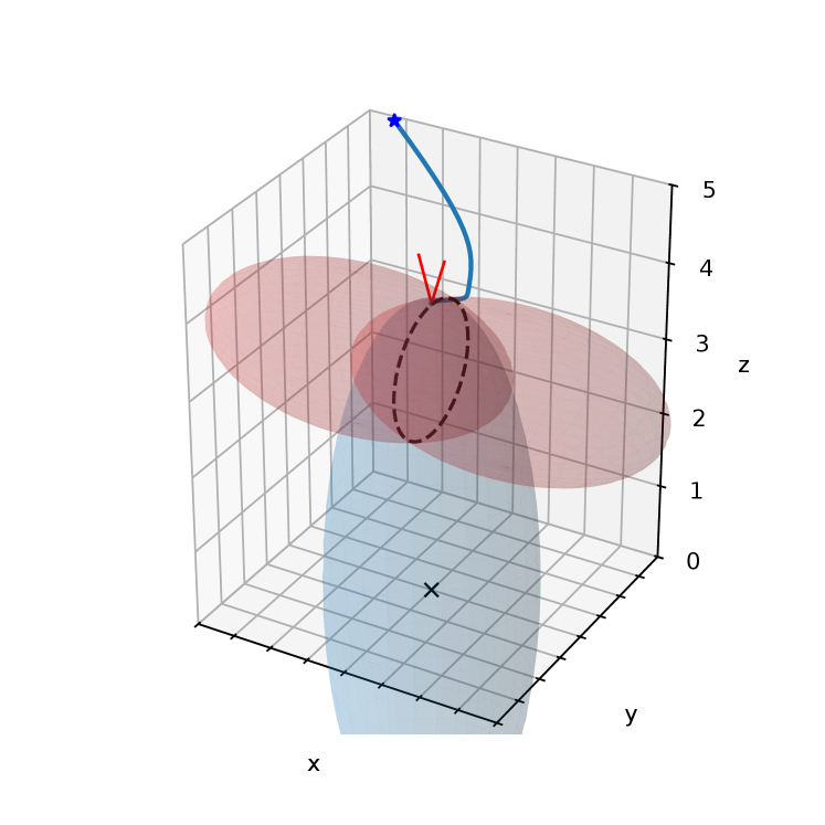
In Fig. 1, we show the simulation result of a safety-critical control task with the CLF-CBF QP-based controller. ¹¹1 The code repository used for producing these results is publicly available at https://github.com/CaipirUltron/CompatibleCLFCBF/tree/mydevel.. Here, $u_{nom}=0$ and $H(x)=I_{3}$ in (3), and the proposed system in $\mathbb{R}^{3}$ is $\dot{x}_{1}=u_{1}-2u_{3}$ , $\dot{x}_{2}=u_{2}$ , $\dot{x}_{3}=-2u_{1}+u_{3}$ . The CBFs are two quadratic functions $h_{1}$ and $h_{2}$ centered at the points $(-1,0,3)$ and $(1,0,3)$ , respectively. Their boundaries are the red ellipsoids in Fig. 1, with the union of their interiors constituting the unsafe set which the system trajectories should avoid. The CLF $V$ is also a quadratic centered on the origin, and its level set is shown in blue, at an asymptotically stable equilibrium point $x_{e}$ at the top of the boundary intersection $\partial\mathcal{C}_{\mathcal{A}}=\partial\mathcal{C}_{1}\cap\partial\mathcal{C}_{2}$ , shown in Fig. 1 by the dashed black circle. A trajectory converging to $x_{e}$ is shown, and the normalized gradients $\nabla h_{1}(x_{e})$ , $\nabla h_{2}(x_{e})$ are shown as the two red vectors pointing up at the equilibrium point. At $x_{e}$ , since $f_{\mathcal{A}}(x_{e},\lambda_{e})=0$ for some $\lambda_{e}=\begin{bmatrix}\,\lambda_{e_{1}}\!&\!\lambda_{e_{2}}\,\end{bmatrix}^{\mathsf{T}}\in\mathbb{R}^{2}_{\geq 0}$ , $f(x_{e})=p\gamma(V(x_{e}))\nabla V(x_{e})-G(x_{e})(\lambda_{e_{1}}\nabla h_{1}(x_{e})+\lambda_{e_{2}}\nabla h_{2}(x_{e}))$ . Since the system is driftless, $f(x)=0\,\,\forall x$ . Furthermore, $G(x_{e})$ is a positive definite matrix. Then, the following holds: $p\gamma(V(x_{e}))\nabla V(x_{e})=\lambda_{e_{1}}\nabla h_{1}+\lambda_{e_{2}}\nabla h_{2}$ , meaning that the gradient of the CLF is a conical combination of the gradients of the active CBFs at $x_{e}$ . That is precisely the case at Fig. 1. Furthermore, due to the fact that the system is driftless with a full rank $G(x_{e})$ , carrying out the needed simplifications at $v^{\mathsf{T}}J_{f_{\mathcal{A}}}(x_{e},\lambda_{e})v$ from (33), one can conclude that the stability of $x_{e}$ is determined by $\lambda_{e_{1}}H_{h_{1}}\!+\!\lambda_{e_{2}}H_{h_{2}}\!-\!p\gamma(V(x_{e}))H_{V}$ , that is, essentially by a difference of curvatures between the CBFs and the CLF at $x_{e}$ , extending the result in [8].

References

[1] Aaron D Ames, Jessy W Grizzle, and Paulo Tabuada. Control barrier function based quadratic programs with application to adaptive cruise control. In 53rd IEEE Conference on Decision and Control, pages 6271–6278. IEEE, 2014.
[2] David ”davidad” Dalrymple et al. Towards guaranteed safe ai: A framework for ensuring robust and reliable ai systems, 2024.
[3] Kai-Chieh Hsu, Haimin Hu, and Jaime F. Fisac. The safety filter: A unified view of safety-critical control in autonomous systems. Annual Review of Control, Robotics, and Autonomous Systems, 7(Volume 7, 2024):47–72, 2024.
[4] Hassan K Khalil. Nonlinear systems; 3rd ed. Prentice-Hall, Upper Saddle River, NJ, 2002.
[5] Taekyung Kim, Robin Inho Kee, and Dimitra Panagou. Learning to refine input constrained control barrier functions via uncertainty-aware online parameter adaptation, 2025.
[6] G. Notomista, S. F. Ruf, and M. Egerstedt. Persistification of robotic tasks using control barrier functions. IEEE Robotics and Automation Letters, 3(2):758–763, April 2018.
[7] Gennaro Notomista and Matteo Saveriano. Safety of dynamical systems with multiple non-convex unsafe sets using control barrier functions. IEEE Control Systems Letters, 6:1136–1141, 2022.
[8] M. F. Reis, A. P. Aguiar, and P. Tabuada. Control barrier function-based quadratic programs introduce undesirable asymptotically stable equilibria. IEEE Control Systems Letters, 5(2):731–736, 2021.
[9] Matheus F. Reis and A. Pedro Aguiar. On the stability of undesirable equilibria in the quadratic program framework for safety-critical control, 2024.
[10] Xiao Tan and Dimos V Dimarogonas. On the undesired equilibria induced by control barrier function based quadratic programs. Automatica, 159:111359, 2024.
[11] Kim P. Wabersich, Andrew J. Taylor, Jason J. Choi, Koushil Sreenath, Claire J. Tomlin, Aaron D. Ames, and Melanie N. Zeilinger. Data-driven safety filters: Hamilton-jacobi reachability, control barrier functions, and predictive methods for uncertain systems. IEEE Control Systems Magazine, 43(5):137–177, 2023.