A Unified Statistical Model for Atmospheric Turbulence-Induced Fading in Orbital Angular Momentum Multiplexed FSO Systems
Abstract
This paper proposes a unified statistical channel model to characterize the atmospheric turbulence induced distortions faced by orbital angular momentum (OAM) in free space optical (FSO) communication systems. In this channel model, the self-channel irradiance of OAM modes as well as crosstalk irradiances between different OAM modes are characterized by a Generalized Gamma distribution (GGD). The latter distribution is shown to provide an excellent match with simulated data for all regimes of atmospheric turbulence. Therefore, it can be used to overcome the computationally complex numerical simulations to model the propagation of OAM modes through atmospheric turbulent FSO channels. The GGD allows obtaining very simple tractable closed-form expressions for a variety of performance metrics. Indeed, the average capacity, the bit-error rate, and the outage probability are derived for FSO systems using single OAM mode transmission with direct detection. Furthermore, we extend our study to FSO systems using OAM mode diversity to improve the performance. By using a maximum ratio combining (MRC) at the receiver, the GGD is also shown to fit the simulated combined received optical powers. Finally, space-time (ST) coding is proposed to provide diversity and multiplexing gains, and the error probability is theoretically derived under the newly proposed generic model.
Index Terms:
Free-space optical communication, orbital angular momentum, atmospheric turbulence, channel modeling, performance analysis, spatial diversity.I Introduction
Space division multiplexing (SDM) technique allows to increase the capacity of a communication system by transmitting several independent data streams in parallel. In optical communications, SDM can be realized by sending different spatial modes in a multi-mode fiber or using many cores in a multi-core fiber [1].
In analogy to optical fiber transmission systems, orbital angular momentum (OAM) is proposed to transmit multiple signals over free space channels [2, 3]. This simultaneous transmission of information on OAM modes is possible thanks to the orthogonality property of OAM beams that allows propagation without interference between signals. A simple scheme of OAM FSO transmission consists in using only the intensity of OAM beams to carry the information. At the receiver, photo-detectors are used to detect light intensity, and the system is operating in intensity-modulation direct-detection (IM/DD). This configuration has a low cost and is more feasible for practical deployment. On the other hand, coherent detection mostly used with optical fibers can also be used for OAM FSO systems. In coherent systems, the spectral efficiency can be further increased by using the two polarizations of light and higher order modulation formats. However, these benefits come at the cost of the high receiver expense and complexity that increases with the number of modes.
By using OAM multiplexing as an additional degree of freedom to polarization and wavelength, coherent laboratory experiment has achieved more than 1 Pbit/s capacity using 26 modes [4].
In real life communication scenarios, transmitted OAM beams are subject to atmospheric turbulence induced distortions that if not properly addressed and compensated may deteriorate the entire FSO link [5, 6, 7]. Several experimental and simulation works have studied the effect of atmospheric turbulence and different techniques to emulate turbulence have been proposed. Atmospheric turbulence can be emulated by using a rotatable phase plate that has a pseudo-random distribution that obeys Kolmogorov statistics. This technique allows to control the turbulence strength and was used in [8], at the transmitter for a 2-OAM transmission in a 100-m round trip FSO link. The same process was used in [9] to emulate turbulence in a 4-OAM modes transmission. An alternative to rotatable phase plate is spatial light modulator (SLM). In fact, the distorted phase hologram of a specific OAM mode after propagation can be generated by computer and printed on a SLM. The latter is used at the receiver as a demodulating SLM that contains the effect of atmospheric turbulence [10]. Besides, propagation of OAM modes through the turbulent atmosphere has also been subject to numerical simulation studies. This can be realized using the split-step Fourier propagation method where turbulence is induced along the propagation path [7, 11, 12, 13, 14]. This technique is very accurate and can simulate the propagation of any OAM mode for different turbulence regimes. Nonetheless, it is computationally complex as it involves many multiplication operations of matrices having large dimensions. Therefore it is important to have a statistical model to describe the propagation of OAM beams in turbulent free space.
In classical FSO systems employing only the Gaussian beam for transmission, several statistical models were proposed for irradiance fluctuations. For example, a Log-Normal distribution can be used to model weak turbulence variations [15]. For moderate, to strong turbulence, a Double-Weibull stochastic model was proposed in [16]. Moreover, the Gamma-Gamma distribution is a widely accepted model used for all levels of turbulence [17]. For all the previous models, closed-form expressions for performance metrics such as the average capacity, the outage probability, and the bit-error rate (BER) were derived.
In OAM FSO systems, to the best of our knowledge, the only proposed statistical channel models for turbulence-induced fading were given in [18, 19]. In this models, the self-channel irradiance of OAM modes was shown to obey a Johnson distribution whereas the crosstalk between OAM modes follows an Exponential distribution. Knowing that the statistical properties of the Johnson distribution are analytically intractable, it is not possible to extract closed-form expressions for performance metrics. Moreover, the lack of a unified turbulence model makes it difficult to assess the effect of the interference on the performance of OAM modes. In [20], the interference fading between OAM modes was assumed to be part of the added Gaussian noise. This consideration has allowed deriving a theoretical BER expression but was unfortunately not corresponding to the numerically simulated BER.
In this work, we show that the Generalized Gamma distribution (GGD) can efficiently model the turbulence induced self-channel fading as well as the crosstalk between OAM modes. The GGD gives a perfect fit for the weak, moderate, and strong turbulence regimes. Closed-form expressions for the outage probability, the average capacity, and the BER are derived for single-input single-output (SISO) transmission using only one OAM mode. Afterward, we consider a multiple-input multiple-output (MIMO) system using several OAM modes to provide diversity gain and hence improve the performance. Furthermore, space-time (ST) coding is proposed to achieve diversity and multiplexing gains, and the corresponding performance is analyzed.
The remainder of this paper is organized as follows. In Section II, we describe the OAM modes generation and propagation in turbulence, and then we present the GGD and its main statistical parameters. In Section III, we compare our proposed GGD model to numerical simulations of atmospheric turbulence fading and also to the Johnson and Exponential models. In Section IV, we derive closed-form expressions for performance metrics using the GGD model and compare the fitting goodness with numerical simulations. Afterward, spatial diversity using several OAM modes is studied and shown to give better performance than SISO links in section V. In section VI, ST coding is proposed to achieve full diversity and multiplexing gains and the theoretical error probability is derived. Finally, the conclusion is given in Section VII.
II Channel Model
II-A Orbital Angular Momentum Multiplexing
By definition, an electromagnetic wave carrying an OAM of per photon is a wave possessing an azimuthally varying phase term , where is an unbounded integer known as the topological charge, is the azimuth and is the reduced Planck constant [21]. To realize OAM multiplexing, single and superposition of orthogonal beams that have a well-defined vorticity can be used including Hermite-Gaussian (HG) beams [22], Ince-Gaussian beams [23], Bessel-Gaussian beams and Laguerre-Gauss (LG) beams [24]. In this work, we are interested in OAM derived from LG modes. The spatial distribution of the LG beams is given by [24]:
| (1) |
where refers to the radial distance. In [24], is the beam radius at the distance , where is the beam waist of the Gaussian beam, is the Rayleigh range, and the optical carrier. In [24], is the propagation constant, is the generalized Laguerre polynomial, where and represent the radial and angular mode numbers. OAM modes correspond to the subset of LG modes having and .
OAM modes generation can be realized in practice by different techniques such as spiral phase plates (SPP) [25], and spatial light modulators (SLM) [26]. An SPP is an optical device that has a spiral staircases form. This geometric shape allows to transform a Gaussian incident beam into a beam with a helical phase front. SPP is an efficient and stable manner to generate OAM beams. However a single SPP allows the generation of only one OAM beam. On the other hand, SLM allows to dynamically generate OAM beams. This is done thanks to computer generated holograms that are printed on the SLM.
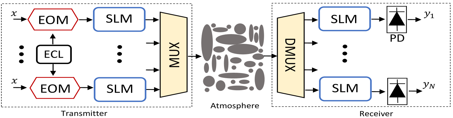
A transmission scheme of OAM FSO system is represented in Fig. 1. The electro-optical modulator (EOM) modulates the signal of the external laser source (ECL). The output optical signal of the EOM is still a Gaussian beam. Thanks to printed holograms, SLMs create the desired OAM modes, then signals are multiplexed and sent into the FSO channel. At the receiver signals are demultiplexed and then inverse operations on the SLMs are performed to convert back signals to Gaussian beams that are detected using the photodiodes. The vorticity of OAM beams propagating in free space without atmospheric turbulence is preserved. Consequently, OAM beams maintain orthogonality as they propagate which can be described by [5, 27]:
| (2) |
where refers to the normalized field distribution of OAM mode of order at the distance and refers to the radial position vector.
II-B OAM Propagation in Turbulence
The propagation of OAM modes can be affected by atmospheric turbulence induced distortions [5, 9, 27, 28]. Atmospheric turbulence is caused by pressure and temperature fluctuations in the atmosphere which result in a random behavior of the atmospheric refractive index [29]. These effects make the atmospheric refractive index to be spatially dependent which distorts the propagating light beams and causes the break of their orthogonality. The spatial fluctuations of the atmospheric refractive index obey a modified Kolmogorov spectrum given by [30]:
| (3) |
where . is the refractive index structure parameter. , with is the outer scale of the turbulence. , with is the inner scale of the turbulence. To emulate atmospheric turbulence, random phase screens are placed along the FSO channel. The strength of the turbulence in a FSO channel is given by the Rytov variance defined as . Weak atmospheric turbulence is usually associated with , whereas strong turbulence refers to [7, 27]. Saturation fluctuations of atmospheric turbulence occurs when [16, 31]. In our work, we define three regimes of atmospheric turbulence depending on the Rytov variance as follows [31]:
| (4) |
Due to atmospheric turbulence, the signal initially launched on an OAM mode will spread to other OAM modes. The leakage of power is more important for adjacent modes to the mode and tends to zero for further OAM modes from mode as shown in [18, 27].
Given that a set of OAM modes can be launched at the transmitter and OAM modes can be detected at the receiver. The transmission of OAM modes in turbulent FSO channel can be described by a multiple-input multiple-output system where the received signal on the OAM mode is given by:
| (5) |
where is the transmitted information bit. is the optical-to-electrical conversion coefficient. is an additive white Gaussian noise with zero mean and variance equal to . represents the fraction of power received on the analyzing field of OAM mode of topological charge when the transmitted power is carried by OAM mode with topological charge . is given by the square of the scalar product between the fields of the two modes as [7, 32]:
| (6) |
was shown to have an Exponential distribution for in [18], and a Johnson distribution for [19]. In the next section we introduce the GGD and present some of its useful statistical properties that we will use latter for performance metrics derivation.
II-C Generalized Gamma Distribution
The GGD was proposed by Stacy in [33]. Its probability density function (PDF) is given by:
| (7) |
where and are the shape parameters, is the scale parameter of the GGD, and denotes the Gamma function. The GGD is a very flexible distribution that includes several well-known distributions. For , Eq. (7) reduces to the Gamma distribution. For , Eq. (7) becomes a Weibull distribution. When , Eq. (7) corresponds to the Exponential distribution. Furthermore, as , Eq. (7) leads to a Log-Normal distribution [34]. By using [35, Eq. (2.9.4)] followed by [35, Eq. (2.1.4)] and [35, Eq. (2.9.1)], we can rewrite the GGD in terms of the Meijer’s G function as:
| (8) |
The cumulative distribution function (CDF) of can be obtained using the definition of the Meijer’s G function in [35, Eq. (2.9.1)]:
| (9) |
The moment of the GGD defined as is given by [34, Eq. (2)]:
| (10) |
where is the expectation operator. The moment generating function (MGF) of the GGD can be derived in terms of the Fox’s H function as [36, Eq. (27)]:
| (11) |
To evaluate the Fox’s H function, an efficient MATHEMATICA implementation can be found in [37, Appendix A]. A simpler expression for the MGF is given in the form of an infinite sum as [33, Eq. (20)]:
| (12) |
III GGD Fitting Comparison with simulations
In this section, we evaluate the suitability of the proposed GGD to fit the simulation data.
As we are working in an IM/DD setup, our Monte Carlo simulations of OAM propagation through the turbulent atmosphere are performed at wavelength nm. The beam waist at the transmitter is cm. On the other hand, the optical receiver is assumed to be large enough to collect all the power on the OAM modes. This condition is satisfied when the receiver diameter is , where is the radius of the Gaussian beam and is the highest OAM topological charge used in the system.
To create the desired OAM modes, SLMs having pixels are used. The propagation distance is set to km, the inner and outer scales of turbulence are set to mm and m, respectively. Atmospheric turbulence is emulated by placing random phase screens each m along the propagation path. Each phase screen is evaluated as the Fourier transform of a complex random distribution with zero mean and variance equal to , where is the array length and mm is the grid spacing assumed to be equal in both dimensions and . Propagation through the turbulent atmosphere is simulated using the commonly used split-step Fourier method [11].
Let be the set of irradiance realizations for a particular and . is the number of samples, where
for each we have simulated realizations. We use a maximum-likelihood (ML) estimation in order to estimate the parameters , , and of . The ML estimator computes the loglikelihood function given by [38]:
| (13) |
The estimated parameters , , and represent the values for which the previous function is maximized and are giving by [38, 39]:
| (14) |
| (15) |
| (16) |
where denotes the digamma function. In our simulations, we have used the ML implementation given in the wafo toolbox [40] .
To validate the goodness of the proposed GGD fit, we used the mean square error (MSE) test. The latter can give a measure on the accuracy of the GGD fitting to the simulated data. The MSE estimator is defined as:
| (17) |
where is the empirical distribution function of and
is the cumulative distribution function of computed using the estimated GGD parameters of .
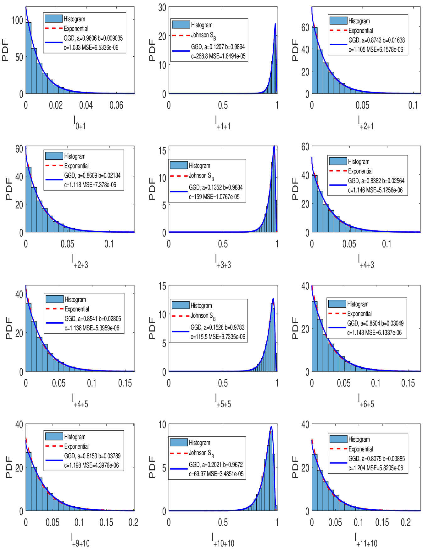
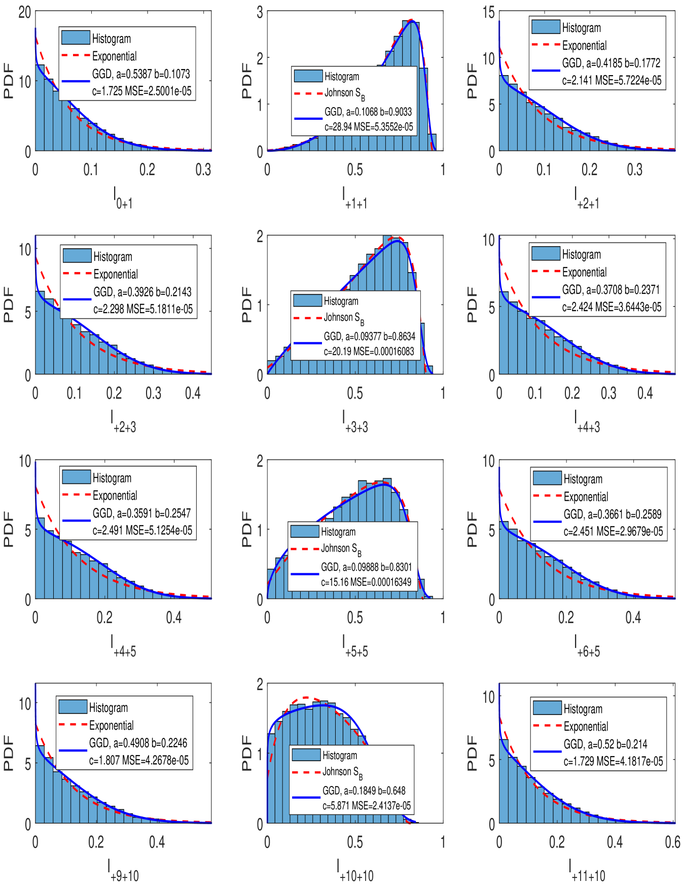
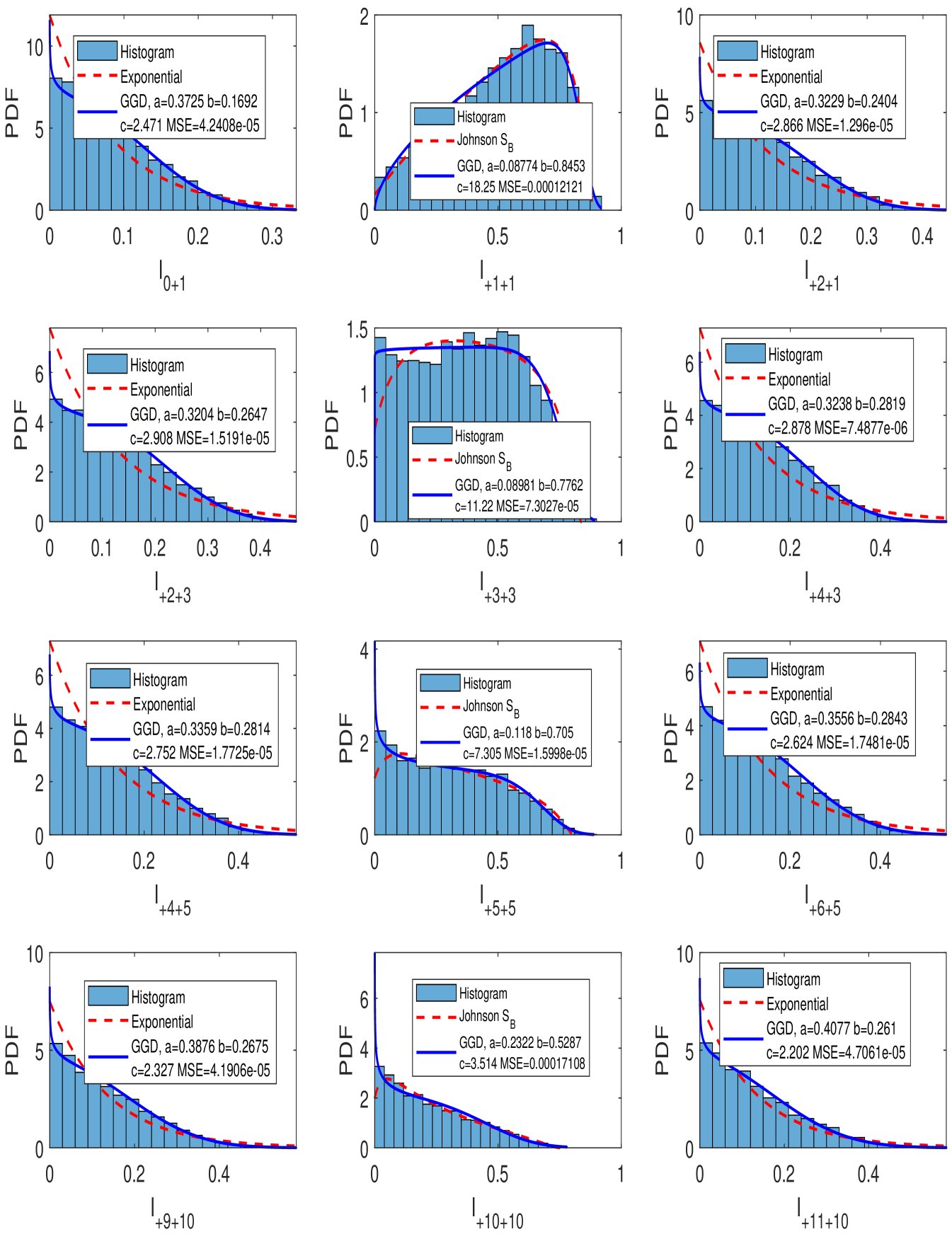
In Figs. 2, 3, and 4, we plot the distributions of for and for different atmospheric turbulence regimes. Also for each distribution, a GGD fitting along with a Johnson or Exponential distribution fitting are plotted.
In Fig. 2, a weak turbulence regime given by and is considered. The center column of the figure shows the obtained results for the self-channel irradiance (i.e., the distribution of the power transmitted on OAM mode and detected on the same OAM mode ). The obtained distributions have a perfect correspondence with the distributions obtained in [18]. The histograms are left skewed and very close to the value of . This is explained by the fact that almost all power transmitted on a specific OAM mode remains in this mode when atmospheric turbulence is weak. Furthermore, we notice that the GGD gives a perfect fit with the obtained histograms and very low values of the MSE were achieved. In addition, the left and right columns of Fig. 2 shows the distribution of the crosstalk of the adjacent OAM modes to the transmitted OAM mode . We notice the Exponential shape of the crosstalk histograms which are perfectly fitted by the GGD, and achieving an MSE always less than .
In Fig. 3, a moderate to strong atmospheric turbulence regime with and is considered. From the center column of Fig. 3, we notice that the effect of turbulence is remarkable on the distributions of which are no longer tight and close to 1. In this regime of turbulence, the GGD is also capable of fitting the simulated data histograms with an MSE less than . For OAM mode , the GGD provides a better fit than the Johnson . In addition, the crosstalk histograms are perfectly fitted by the GGD and its fitting is also much better than the Exponential fit. Lastly, for the saturation regime, we have considered and . As for the previous two cases, the GGD gives an excellent fit for all the obtained distributions and achieves a very low MSE. Moreover, for the crosstalk distributions, we notice from Fig. 4 that the GGD gives a better fit than the Exponential fit. Consequently, all the previous results indicate that the GGD is a very suitable candidate to model the irradiance distributions of OAM FSO transmission systems in the presence of atmospheric turbulence. Furthermore, we also notice from Figs. 2, 3, and 4 that the parameters , , and of the GGD depend on the OAM mode as well as the atmospheric turbulence strength. This situation is more complex than the classical FSO systems where the parameters of the irradiance of the Gaussian beam modeled as a Gamma-Gamma distribution could be directly derived from the inner and outer scale of the atmospheric turbulence [17]. Consequently, the computation of the parameters of the GGD in OAM FSO systems as a function of the OAM mode order and the turbulence strength is subject of future works.
IV Performance Analysis of SISO OAM Links
In this section, we consider that only one OAM mode is transmitted and detected in a system operating in intensity modulation and direct detection. For notational convenience, we omit the subscript and refer to by . The instantaneous electrical signal-to-noise ratio (SNR) is defined as . The average electrical SNR is defined as . After a simple power transformation of the variable in Eq. (8), the PDF of the instantaneous SNR can be written as:
| (18) |
The CDF of the SNR defined as: can be obtained using the Meijer’s G function definition in [35, Eq. (2.9.1)]:
| (19) |
Now that we have defined the PDF and CDF of the SNR, we can proceed to the performance metrics derivation.
IV-A Ergodic Capacity
IV-B Outage Probability
The outage probability is the probability that the instantaneous SNR falls bellow an SNR threshold that ensures a reliable communication. It is given by the CDF of evaluated at the value as:
| (22) |
IV-C Average BER
IV-D Numerical Simulations Evaluation
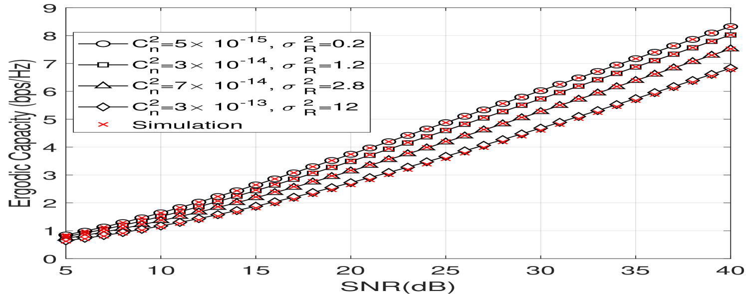
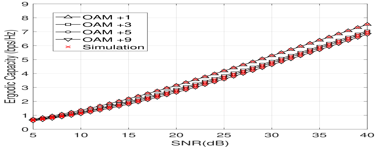
In this section, numerical simulations of the previous defined performance metrics are presented and compared to Monte Carlo simulations. In Fig. 5(a), we plot the ergodic capacity as a function of the average SNR for the SISO link using OAM mode for different levels of atmospheric turbulence. From the figure, we notice that the capacity decreases with increasing turbulence. Furthermore, we clearly observe that the analytical capacity curves have a perfect match with the simulated capacities which confirms the accuracy of our derivations. In Fig. 5(b), we compare the ergodic capacities using different OAM modes for the moderate to strong turbulence regime given by and . The highest capacity is obtained for OAM mode followed by other OAM modes having slightly the same capacity. This can be explained by the fact that OAM mode is the less affected by atmospheric turbulence and as shown from Fig. 2 the power distribution of OAM mode remains mostly in the same mode.
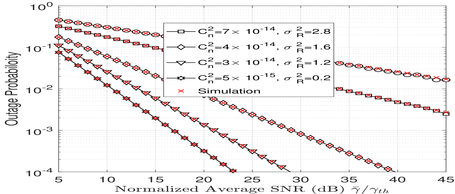
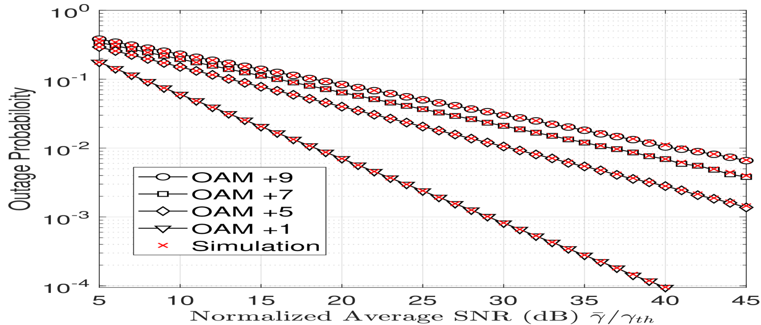
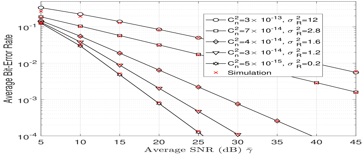
The outage probability of OAM mode is presented in Fig. 6(a) as a function of the normalized average SNR for different levels of atmospheric turbulence. From the figure, we notice that the outage probability increases with increasing atmospheric turbulence which degrades the performance. For example, at a normalized average SNR of 20 dB, when the Rytov variance is , and for , . In Fig. 6(b), we compare the outage probabilities obtained by different OAM modes for a moderate to strong atmospheric turbulence regime with and . From the figure, we notice that the lowest outage performance is reached by OAM mode and as the OAM mode order increases the outage performance degrades.
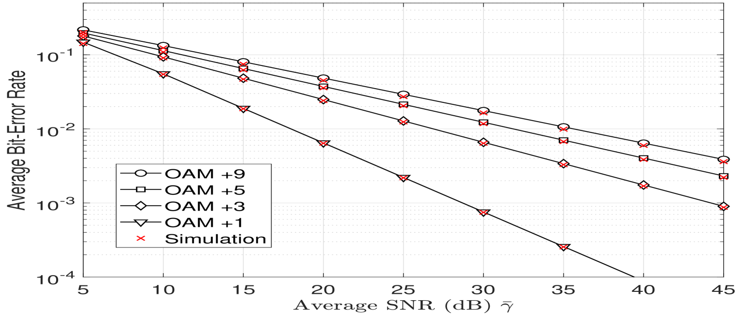
In Fig. 7(a) and 7(b), the average BER is plotted as a function of the average SNR for different OAM modes and at several levels of atmospheric turbulence. From the figures, we can notice an excellent match between theoretical results and simulations, and as for the outage probability, OAM mode achieves the lowest BER performance. Consequently, from all the previously obtained results, the proposed analytical performance metrics derived from the GGD are very accurate and perfectly match numerical simulations.
V MIMO OAM Links with Spatial Diversity
In this section, we propose to enhance the error performance of OAM FSO systems by using multiple OAM beams to transmit the same data. Typically, FSO systems have used multiple transmitters and receivers having apertures that are separated enough to bring diversity gain [44, 45]. However, this strategy comes at the cost of more hardware complexity and apertures spacing limitations which cannot always be satisfied. Spatial diversity can be used at the receiver in the form of a single-input multiple-output (SIMO) system as in [27]. At the receiver, combining techniques such as equal gain combining (EGC), selective combining (SC) or maximum ratio combining (MRC) can be used. Spatial diversity can also be set at the transmitter in the form of a multiple-input single-output (MISO) system [46]. In this case, beamforming can be used thanks to channel state information to improve the performance [47]. Moreover OAM mode selection can also be used to achieve better rates and lower BER [14, 27]. In the absence of channel state information, space-time coding can also be used as an alternative solution to increase the performance [14]. Spatial diversity can be used at both the transmitter and the receiver in the form of a MIMO system [46]. We consider a square MIMO system where OAM modes are transmitted and received. By using a MRC at the receiver, the electrical SNR is given by [46, Eq. (14)]:
| (25) |
where the factor in the previous equation allows to compare the SISO and MIMO systems at the same transmitted optical power.
The derivation of the exact PDF of is complex as it involves sums of GGDs that are non identically distributed. To overcome this issue and compare the performance of SISO and MIMO configurations, we approximate by a GGD and estimate its parameters. Therefore, the PDF and CDF of can be directly given from Eq. (18) and Eq. (19), and the outage probability and average BER can be theoretically computed using Eq. (22) and Eq. (24).
Before performance evaluation of the MIMO system, it is important to choose the appropriate OAM modes in order to fully exploit the benefit of the spatial diversity. When an OAM mode of order is used for transmission, it is normal to detect the power conserved in that mode first. In fact, the power is much higher than the power spread into other modes given by as shown from Figs. 2, 3, and 4.
When using spatial diversity, the detected signal on OAM mode contains the power transmitted from OAM mode and also crosstalk powers from other transmitted OAM modes as given by Eq. (5).
Furthermore, the performance achieved by the spatial diversity is limited by the correlation between spatial paths [44]. Therefore, to achieve the maximum spatial diversity gain, the correlation between the self-channel irradiance and the crosstalk has to be minimal. To have an insight on the correlation between OAM modes, we propose to compute the correlation coefficient between and given by:
| (26) |
where is the covariance and is the standard deviation.
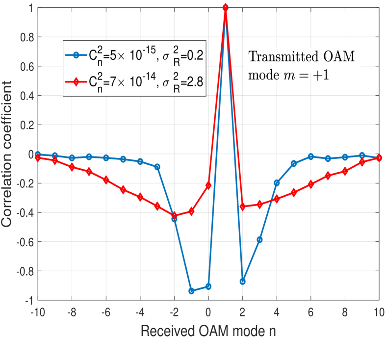
Consider that OAM mode is transmitted, we compute the correlation coefficients between and for . In Fig. 8, we plot the correlation coefficients for the weak (resp. strong) turbulence regimes given by and (resp. and ). From Fig. 8, we notice that adjacent modes to the transmitted mode have inverse correlation coefficient. The latter increases as the mode order gets further from . Therefore, closer OAM mode orders are preferred to achieve a maximum diversity [27]. In addition to the correlation, the power spread from the transmitted mode due to atmospheric turbulence is more important for adjacent OAM modes than further modes. Therefore, higher SNR gain will be provided by using modes with closer OAM order.
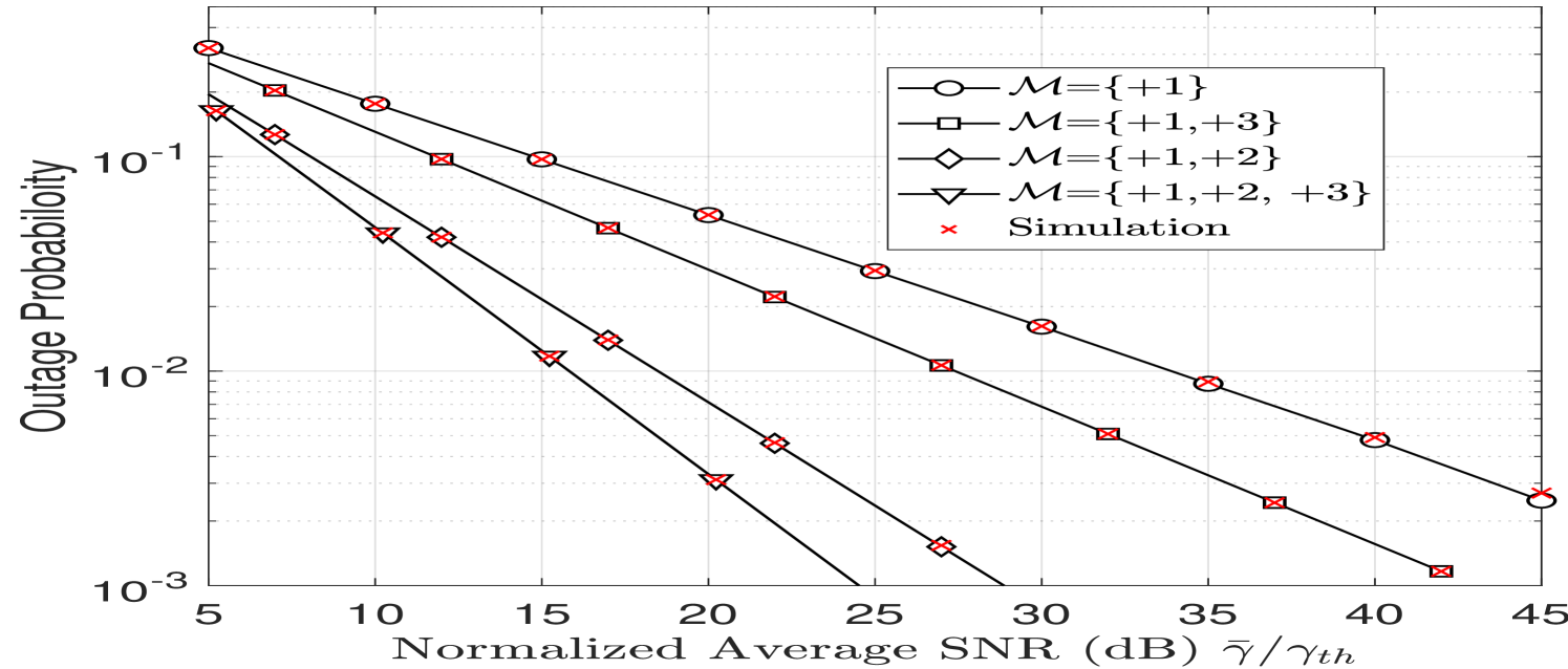
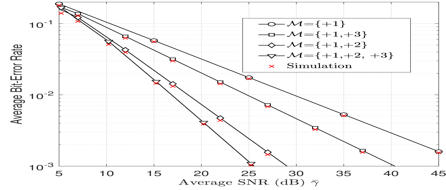
In Fig. 9, the performance of OAM FSO system using spatial diversity is presented for the moderate to strong turbulence regime given by and . For both the outage probability and the average BER, we notice that the set achieves better performance than the set as expected. Furthermore, increasing the number of OAM modes enhances the performance as shown from the curve with the set . In addition, we have also approximated with a GGD and estimated its parameters which allowed to compute the theoretical outage probability and average BER. The plotted curves based on the GGD approximation give an excellent match with the simulated data.
VI Space-Time Coding for OAM FSO Systems
In the previous section, we have shown that spatial diversity can improve the error performance by sending multiple replicas of the same signal on different OAM modes. Nonetheless, the achieved diversity performance was obtained at the cost of a reduced multiplexing gain. To achieve full diversity and multiplexing gains, we consider space-time coding. ST coding was originally designed for wireless radio-frequency (RF) systems [48], and recently investigated for few-mode fibers [49, 50]. The Golden code [51] was designed for wireless MIMO systems and achieves a full diversity with the best coding gain for Rayleigh fading channels. The Alamouti code [52], is a half-rate orthogonal ST code that also achieves a full diversity and has the benefit of a very low decoding complexity that reduces to a simple channel inversion. ST coding was also demonstrated with heterodyne multiple apertures FSO systems [53]. However, due to the high cost of heterodyne implementation and complex signal processing required for ST decoding, it is not easily deployed in practice.
In addition, ST coding was also investigated for multiple apertures IM/DD FSO systems. In [54], a theoretical error probability was derived, and ST coding was shown to achieve full diversity. Furthermore, modified versions of known ST codes from RF were constructed and adapted to IM/DD systems. In [55, 56] modified versions of the Alamouti code were proposed. The new constructed Alamouti code preserves all the useful properties of the original code. The codeword matrix of the Alamouti code is given by [55]:
| (27) |
where the symbol refers to the bit-wise not of the transmitted bit . The main drawback of the Alamouti code is its half-rate code that only allows sending two bits during two time slots and using two OAM modes.
Furthermore, Mroueh has proposed the Golden-Light (GL) code [57] which is an extended version of the Golden code that was adapted to IM/DD systems. The proposed code was shown to conserve an optimal and non-vanishing determinant. The GL codeword is given by [57]:
| (28) |
where and are specific algebraic numbers related to the code construction. In addition to a full diversity, The GL code has a full-rate, which means that during two time slots and using two OAM modes, the GL code allows transmitting four bits .
To evaluate the performance of ST coding in OAM FSO systems affected by atmospheric turbulence, we consider that OAM modes are transmitted and detected. The resulting MIMO transmission system is given by:
| (29) |
where and are the transmitted and received codewords. represents an additive white Gaussian noise with zero mean and a variance per complex dimension. represents the channel matrix with entries . In the next section, we derive a theoretical expression of the error probability of ST coded OAM FSO systems.
VI-A Derivation of the Error Probability
Let be the transmitted codeword and the estimated codeword. Considering a maximum-likelihood decoder, the error probability is defined as:
| (30) |
For equiprobable codewords and using the union bound of the error probability [58], we obtain:
| (31) |
where is the set of all possible codewords and is the average pairwise error probability (PEP) of transmitting and decoding . Let denotes the difference of two codewords, the evaluation of the error probability simplifies to the averaging of the conditional PEP given by [54]:
| (32) |
| (33) | ||||
| (34) |
where . is a hermitian matrix, thus there exists a unitary matrix and a real diagonal matrix such that , hence:
| (35) |
with . By injecting the previous equation in Eq. (32) and using the definition of the function, the pairwise error probability becomes:
| (36) |
where we have denoted .
A further derivation of the previous equation requires the knowledge about the distribution of which is not accessible due to the terms .
However, in the case of orthogonal ST codes we have [59], where , and are the elements of the matrix and is the two dimensional identity matrix. Therefore in the case of orthogonal ST codes, Eq. (36) becomes:
| (37) |
As detailed in the previous section, the fading coefficients are not independent. Hence, it is not possible to apply the approach used in [48] that consists in taking the average of the conditional pairwise error probability and writing the moment of the product as the product of moments. To overcome this, we approximate the random variable with a GGD. Therefore, the SNR of orthogonal ST codes can be written as . Hence, the average pairwise error probability of orthogonal ST codes becomes:
| (38) |
VI-B Numerical Results
We consider a MIMO system using the set of OAM modes , and we compare the performance obtained by using ST coding to the spatial diversity. To make a fair comparison between the different schemes, we compare the BER performances at the same transmitted bits per channel use (bpcu). For this purpose, we use an L-aray pulse amplitude modulation (PAM). In the case of the GL code, it is possible to send 4 modulated symbols during 2 time slots. We use a 2-PAM modulation to obtain a rate of 2 bpcu. To satisfy the same rate, we use a 4-PAM modulation in the case of the Alamouti code and the spatial diversity scheme.
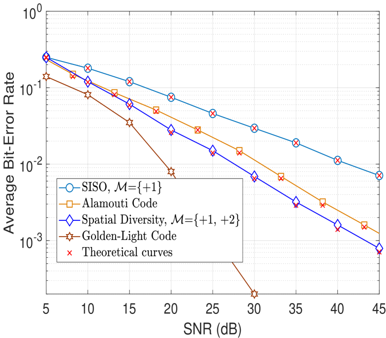
In Fig. 10, we plot the obtained BER performance. The SISO link using OAM mode is also plotted as a reference. From the figure, we notice that the GL code outperforms all other schemes. This is due to the coding gain of the GL code and also the use of the 2-PAM modulation instead of the 4-PAM for other schemes. Moreover, we notice that the spatial diversity scheme outperforms the Alamouti code which is consistent with the previous results obtained in [55, 60]. In addition, the theoretical performance of the Alamouti code based on the GGD approximation has a good match with the simulated performance.
VII Conclusion
In this paper, we have proposed a new statistical model for atmospheric turbulence fading in OAM FSO transmission systems. The proposed GGD can model the self-channel irradiance of OAM modes as well as the crosstalk between OAM modes for all atmospheric turbulence regimes. Hence, the proposed model can be used to overcome the computationally complex Monte Carlo simulations to simulate the propagation of OAM beams. Afterward, we have derived analytical expressions for the ergodic capacity, the outage probability, and the average BER. The obtained results show perfect match with simulations. Moreover, we have proposed to enhance the performance of OAM FSO systems by considering spatial diversity where several OAM modes are used to transmit the same data. From the obtained outage probability and average BER, significant performance improvements were achieved. Finally, ST coding was proposed to achieve full diversity and multiplexing gains. A theoretical derivation of the error probability was conducted, and numerical simulations of different ST codes were presented.
References
- [1] D. J. Richardson, J. M. Fini, and L. E. Nelson, “Space-division multiplexing in optical fibres,” Nature Photonics, vol. 7, no. 5, pp. 354, 2013.
- [2] A. E. Willner, J. Wang, and H. Huang, “A different angle on light communications,” Science, vol. 337, no. 6095, pp. 655–656, 2012.
- [3] A. Trichili, K.-H. Park, M. Zghal, B. S. Ooi, and M.-S. Alouini, “Communicating using spatial mode multiplexing: Potentials, challenges and perspectives,” accepted for publication in IEEE Communications Surveys & Tutorials, 2019.
- [4] J. Wang, S. Li, M. Luo, J. Liu, L. Zhu, C. Li, D. Xie, Q. Yang, S. Yu, and J. Sun, “N-dimentional multiplexing link with 1.036-pbit/s transmission capacity and 112.6-bit/s/Hz spectral efficiency using OFDM-8QAM signals over 368 WDM pol-muxed 26 OAM modes,” in European Conference on Optical Communication (ECOC), 2014, pp. 1–3.
- [5] Y. Ren, G. Xie, H. Huang, N. Ahmed, Y. Yan, L. Li, C. Bao, M. PJ. Lavery, M. Tur, and M. A. Neifeld, “Adaptive-optics-based simultaneous pre-and post-turbulence compensation of multiple orbital-angular-momentum beams in a bidirectional free-space optical link,” Optica, vol. 1, no. 6, pp. 376–382, 2014.
- [6] M. Li, M. Cvijetic, Y. Takashima, and Z. Yu, “Evaluation of channel capacities of OAM-based FSO link with real-time wavefront correction by adaptive optics,” Optics Express, vol. 22, no. 25, pp. 31337–31346, 2014.
- [7] J. A Anguita, M. A Neifeld, and B. V Vasic, “Turbulence-induced channel crosstalk in an orbital angular momentum-multiplexed free-space optical link,” Applied Optics, vol. 47, no. 13, pp. 2414–2429, 2008.
- [8] L. Li, R. Zhang, P. Liao, Y. Cao, H. Song, Y. Zhao, J. Du, Z. Zhao, C. Liu, K. Pang, H. Song, D. Starodubov, B. Lynn, R. Bock, M. Tur, A. F. Molisch, and A. E. Willner, “MIMO equalization to mitigate turbulence in a 2-channel 40-Gbit/s QPSK free-space optical 100-m round-trip orbital-angular-momentum-multiplexed link between a ground station and a retro-reflecting UAV,” in 2018 European Conference on Optical Communication (ECOC), 2018, pp. 1–3.
- [9] H. Huang, Y. Cao, G. Xie, Y. Ren, Y. Yan, C. Bao, N. Ahmed, M. A Neifeld, S. J. Dolinar, and A. E. Willner, “Crosstalk mitigation in a free-space orbital angular momentum multiplexed communication link using 44 MIMO equalization,” Optics Letters, vol. 39, no. 15, pp. 4360–4363, 2014.
- [10] T. Sun, M. Liu, Y. Li, and M. Wang, “Crosstalk mitigation using pilot assisted least square algorithm in OFDM-carrying orbital angular momentum multiplexed free-space-optical communication links,” Optics Express, vol. 25, no. 21, pp. 25707–25718, 2017.
- [11] A. Belmonte, “Feasibility study for the simulation of beam propagation: Consideration of coherent Lidar performance,” Applied Optics, vol. 39, no. 30, pp. 5426–5445, 2000.
- [12] S. Zhao, J. Leach, L.Y. Gong, J. Ding, and B.Y. Zheng, “Aberration corrections for free-space optical communications in atmosphere turbulence using orbital angular momentum states,” Optics Express, vol. 20, no. 1, pp. 452–461, 2012.
- [13] X. Liu and J. Pu, “Investigation on the scintillation reduction of elliptical vortex beams propagating in atmospheric turbulence,” Optics Express, vol. 19, no. 27, pp. 26444–26450, 2011.
- [14] E.-M. Amhoud, A. Trichili, B. S. Ooi, and M.-S. Alouini, “OAM mode selection and space-time coding for turbulence mitigation in FSO communications,” IEEE Access, vol. 7, pp. 88049–88057, 2019.
- [15] A.M. Obukhov, “Effect of weak inhomogeneities in the atmosphere on sound and light propagation,” Izv. Akad. Nauk. Seriya Geofiz, vol. 2, pp. 155–165, 1953.
- [16] N. D. Chatzidiamantis, H. G. Sandalidis, G. K. Karagiannidis, S. A Kotsopoulos, and M. Matthaiou, “New results on turbulence modeling for free-space optical systems,” in IEEE 17th International Conference on Telecommunications, 2010, pp. 487–492.
- [17] A. Al-Habash, L. C. Andrews, and R. L. Phillips, “Mathematical model for the irradiance probability density function of a laser beam propagating through turbulent media,” Optical Engineering, vol. 40, no. 8, pp. 1554–1563, 2001.
- [18] J. A. Anguita, M. A. Neifeld, and B. V. Vasic, “Modeling channel interference in an orbital angular momentum-multiplexed laser link,” in Free-Space Laser Communications IX. Intern. Soc. for Optics and Photonics, 2009, vol. 7464, p. 74640U.
- [19] G. Funes, M. Vial, and J. A. Anguita, “Orbital-angular-momentum crosstalk and temporal fading in a terrestrial laser link using single-mode fiber coupling,” Optics Express, vol. 23, no. 18, pp. 23133–23142, 2015.
- [20] M. Alfowzan, J. A. Anguita, and B. Vasic, “Joint detection of multiple orbital angular momentum optical modes,” in Global Communications Conference (GLOBECOM), 2013, pp. 2388–2393.
- [21] L. Allen, M. W Beijersbergen, R. Spreeuw, and J. P. Woerdman, “Orbital angular momentum of light and the transformation of Laguerre-Gaussian laser modes,” Physical Review A, vol. 45, no. 11, pp. 8185, 1992.
- [22] W. C. Soares, D. P. Caetano, and J. M. Hickmann, “Hermite-Bessel beams and the geometrical representation of nondiffracting beams with orbital angular momentum,” Optics Express, vol. 14, no. 11, pp. 4577–4582, 2006.
- [23] M. A. Bandres and J. C. Gutiérrez-Vega, “Ince–Gaussian beams,” Optics Letters, vol. 29, no. 2, pp. 144–146, 2004.
- [24] T. Doster and A. T. Watnik, “Laguerre–Gauss and Bessel–Gauss beams propagation through turbulence: Analysis of channel efficiency,” Applied Optics, vol. 55, no. 36, pp. 10239–10246, 2016.
- [25] M. Massari, G. Ruffato, M. Gintoli, F. Ricci, and F. Romanato, “Fabrication and characterization of high-quality spiral phase plates for optical applications,” Applied Optics, vol. 54, no. 13, pp. 4077–4083, 2015.
- [26] Y. Ohtake, T. Ando, N. Fukuchi, N. Matsumoto, H. Ito, and T. Hara, “Universal generation of higher-order multiringed Laguerre-Gaussian beams by using a spatial light modulator,” Optics Letters, vol. 32, no. 11, pp. 1411–1413, 2007.
- [27] S. Huang, G. R. Mehrpoor, and M. Safari, “Spatial-mode diversity and multiplexing for FSO communication with direct detection,” IEEE Transactions on Communications, vol. 66, no. 5, pp. 2079–2092, 2018.
- [28] Y. Ren, Z. Wang, G. Xie, L. Li, A. J. Willner, Y. Cao, Z. Zhao, Y. Yan, N. Ahmed, and N. Ashrafi, “Atmospheric turbulence mitigation in an OAM-based MIMO free-space optical link using spatial diversity combined with MIMO equalization,” Optics Letters, vol. 41, no. 11, pp. 2406–2409, 2016.
- [29] B. Rodenburg, M. P.J. Lavery, M. Malik, M. N. O’Sullivan, M. Mirhosseini, D. J. Robertson, M. Padgett, and R. W. Boyd, “Influence of atmospheric turbulence on states of light carrying orbital angular momentum,” Optics Letters, vol. 37, no. 17, pp. 3735–3737, 2012.
- [30] L C. Andrews, “An analytical model for the refractive index power spectrum and its application to optical scintillations in the atmosphere,” Journal of Modern Optics, vol. 39, no. 9, pp. 1849–1853, 1992.
- [31] T. D. Katsilieris, G. P. Latsas, H. E. Nistazakis, and G. S. Tombras, “An accurate computational tool for performance estimation of FSO communication links over weak to strong atmospheric turbulent channels,” Computation, vol. 5, no. 1, pp. 18, 2017.
- [32] G. R. Mehrpoor, M. Safari, and B. Schmauss, “Free space optical communication with spatial diversity based on orbital angular momentum of light,” in 4th International Workshop on Optical Wireless Communications, 2015, pp. 78–82.
- [33] E. W. Stacy, “A generalization of the gamma distribution,” The Annals of Mathematical Statistics, vol. 33, no. 3, pp. 1187–1192, 1962.
- [34] M. Khodabina and A. Ahmadabadib, Some properties of generalized gamma distribution, Mathematical Sciences, 2010.
- [35] A. Kilbas and M. Saigo, H-transforms: Theory and Applications, CRC Press, 2004.
- [36] E. Zedini, H. M. Oubei, A. Kammoun, M. Hamdi, B. S. Ooi, and M.-S. Alouini, “Unified statistical channel model for turbulence-induced fading in underwater wireless optical communication systems,” IEEE Transactions on Communications, vol. 67, no. 4, pp. 2893–2907, 2019.
- [37] F. Yilmaz and M.-S. Alouini, “Product of the powers of generalized Nakagami-m variates and performance of cascaded fading channels,” in IEEE Global Telecommunications Conference, 2009, pp. 1–8.
- [38] J. Y. Wong, “Simultaneously estimating with ease the three parameters of the generalized gamma distribution,” Microelectronics Reliability, vol. 33, no. 15, pp. 2233–2242, 1993.
- [39] K.-S. Song, “Globally convergent algorithms for estimating generalized gamma distributions in fast signal and image processing,” IEEE Transactions on Image Processing, vol. 17, no. 8, pp. 1233–1250, 2008.
- [40] http://www.maths.lth.se/matstat/wafo/documentation/wafodoc/wafo/wstats/index.html.
- [41] A. Lapidoth, S. M. Moser, and M. Wigger, “On the capacity of free-space optical intensity channels,” IEEE Transactions on Information Theory, vol. 55, no. 10, pp. 4449–4461, 2009.
- [42] A. Chaaban, J.-M. Morvan, and M.-S. Alouini, “Free-space optical communications: Capacity bounds, approximations, and a new sphere-packing perspective,” IEEE Transactions on Communications, vol. 64, no. 3, pp. 1176–1191, 2016.
- [43] E. Zedini, H. Soury, and M.-S. Alouini, “Dual-hop FSO transmission systems over Gamma–Gamma turbulence with pointing errors,” IEEE Transactions on Wireless Communications, vol. 16, no. 2, pp. 784–796, 2017.
- [44] S. M. Navidpour, M. Uysal, and M. Kavehrad, “BER performance of free-space optical transmission with spatial diversity,” IEEE Transactions on Wireless Communications, vol. 6, no. 8, pp. 2813–2819, 2007.
- [45] M.-A. Khalighi, N. Schwartz, N. Aitamer, and S. Bourennane, “Fading reduction by aperture averaging and spatial diversity in optical wireless systems,” IEEE Journal of Optical Communications and Networking, vol. 1, no. 6, pp. 580–593, 2009.
- [46] T. A. Tsiftsis, H. G. Sandalidis, G. K. Karagiannidis, and M. Uysal, “Optical wireless links with over strong atmospheric turbulence channels,” IEEE Transactions on Wireless Communications, vol. 8, no. 2, pp. 951–957, 2009.
- [47] S. Huang and M. Safari, “Spatial-mode multiplexing with zero-forcing beamforming in free space optical communications,” in IEEE International Conference on Communications Workshops, 2017, pp. 331–336.
- [48] V. Tarokh, N. Seshadri, and A. R. Calderbank, “Space-time codes for high data rate wireless communication: Performance criterion and code construction,” IEEE Transactions on Information Theory, vol. 44, no. 2, pp. 744–765, 1998.
- [49] E-M. Amhoud, R. Rekaya, L. Bigot, M. Song, E. R. Andresen, G. Labroille, M. Bigot-Astruc, and Y Jaouen, “Experimental demonstration of space-time coding for mdl mitigation in few-mode fiber transmission systems,” in IEEE European Conference on Optical Communication (ECOC), 2017, pp. 1–3.
- [50] E-M. Amhoud, G. Rekaya, and Y. Jaouen, “Design criterion of space-time codes for sdm optical fiber systems,” in 23rd International Conference on Telecommunications (ICT), 2016, pp. 1–5.
- [51] J.-C. Belfiore, G. Rekaya, and E. Viterbo, “The Golden code: A full-rate space-time code with nonvanishing determinants,” IEEE Transactions on Information Theory, vol. 51, no. 4, pp. 1432–1436, 2005.
- [52] S. M. Alamouti, “A simple transmit diversity technique for wireless communications,” IEEE Journal on Selected Areas in Communications, vol. 16, no. 8, pp. 1451–1458, 1998.
- [53] S. M. Haas, J. H. Shapiro, and V. Tarokh, “Space-time codes for wireless optical communications,” EURASIP Journal on Applied Signal Processing, vol. 2002, no. 1, pp. 211–220, 2002.
- [54] E. Bayaki and R. Schober, “On space-time coding for free-space optical systems,” IEEE Transactions on Communications, vol. 58, no. 1, pp. 58–62, 2010.
- [55] M. Safari and M. Uysal, “Do we really need OSTBCs for free-space optical communication with direct detection?,” IEEE Transactions on Wireless Communications, vol. 7, no. 11, pp. 4445–4448, 2008.
- [56] M. K. Simon and V. A. Vilnrotter, “Alamouti-type space-time coding for free-space optical communication with direct detection,” IEEE Transactions on Wireless Communications, vol. 4, no. 1, pp. 35–39, 2005.
- [57] L. Mroueh, “Extended Golden light code for FSO-MIMO communications with time diversity,” IEEE Transactions on Communications, vol. 67, no. 1, pp. 553–563, 2019.
- [58] J. G. Proakis and M. Salehi, Digital Communications, McGraw-Hill, Fifth Edition, Chapter 4, 2008.
- [59] O. Tirkkonen and A. Hottinen, “Square-matrix embeddable space-time block codes for complex signal constellations,” IEEE Transactions on Information Theory, vol. 48, no. 2, pp. 384–395, 2002.
- [60] Y. Sapenov, A. Chaaban, Z. Rezki, M. Abdallah, K. Qaraqe, and M.-S. Alouini, “Diversity order results for MIMO optical wireless communications,” IEEE Wireless Communications Letters, vol. 7, no. 1, pp. 74–77, 2018.