A Uniformly Most Powerful Unbiased Test for Regression Parameters by Orthogonalizing Predictors

It is well known from practice that having correlated predictors in a multiple regression model leads to loss of power. In an extreme case, including perfectly correlated predictors leads to a model that is over-identified. Even if features are highly, but not perfectly, correlated, multicollinearity might make the model fit unstable. The amount of multicollinearity is sometimes measured via variance inflation factors (VIFs). Parameters that have high VIF are deemed to significantly increase multicollinearity of the model and might be excluded. However, sometimes it is desirable to keep related predictors as each might contain unique information.

Orthogonalizing the design matrix is an alternative way to deal with the multicollinearity problem. This is not a new concept, having been used in many ways in many fields, see, e.g., [3, 4]. Orthogonalizing the feature space via principal components or other methods (e.g., [8]) is a standard choice as a dimension reduction technique, especially when the number of features is large, and when interpretability is not particularly important. By contrast, uptake of this approach is limited, even non-existent, when the feature space is made up of a smaller number of meaningful predictors. This may be due to the open-ended modeling questions that it raises, namely, in which order to orthogonalize features, and how to interpret the newly created predictor set. In this paper we orthogonalize features sequentially, preserving the dimension of the design matrix, and select the new basis starting from one of the initial predictors as the first direction. We do this both for ease of interpretation, and because we want to increase power in testing the significance of one predictor that may be of particular importance in a multiple regression problem. Section 2 introduces the two main theoretical results of the paper. In Section 3, we show on a simulated example that power gains can be significant if the features are correlated, and we conclude in Section 4 with a discussion of where this approach might be most beneficial and how the new features might be interpreted.

We introduce the main result, which concerns the one-sided test of a coefficient in a multiple regression model, where features are orthonormal. The proof generalizes Example 6.9.11 from [1] , which establishes the result in the more limited case of testing for the slope in a simple regression model in which intercept and error variance are unknown.

THEOREM 1. Suppose we observe data vector $\mathbf{Y}$ from the multiple regression model $\bm{Y}=\beta_{1}\mathbf{x}_{1}+\beta_{2}\mathbf{x}_{2}+...+\beta_{p}\mathbf{x}_{p}+\bm{\epsilon}$, where $\bm{\epsilon}\sim N(0,\sigma^{2}I),$ and $\mathbf{x_{1},x_{2},...,x_{p}}$ are fixed covariates, for $p<n$. Assume further that $\mathbf{x_{1},x_{2},...,x_{p}}$ form an orthonormal basis for $\mathbb{R}^{p}$, and all parameters ($\beta_{1},\beta_{2},...,\beta_{p}$ and $\sigma^{2}$) are unknown. The test $\phi$ defined as

where $V=\frac{\sqrt{n-p}\,\mathbf{x}_{p}^{\intercal}\mathbf{Y}}{\sqrt{\mathbf{Y}^{\intercal}\mathbf{Y}-\sum_{i=1}^{p}{(\mathbf{x}_{i}^{\intercal}\mathbf{Y})^{2}}}}\sim t_{n-p}$ is UMPU for testing $H_{0}:\beta_{p}\leq 0$ vs $H_{1}:\beta_{p}>0$.

PROOF: As is typical when looking for a UMP test in the presence of nuisance parameters, we first wish to identify sufficient statistics for this inference. With normal data, the joint density will belong to the exponential family and can be written thus

From this, the sufficient statistics are $(\mathbf{Y}^{\intercal}\mathbf{Y},\mathbf{x}_{1}^{\intercal}\mathbf{Y},\mathbf{x}_{2}^{\intercal}\mathbf{Y},...,\mathbf{x}_{p}^{\intercal}\mathbf{Y})$ corresponding to the natural parameter vector $(-\frac{1}{2\sigma^{2}},\frac{\beta_{1}}{2\sigma^{2}},...,\frac{\beta_{p}}{2\sigma^{2}})$. According to [1] (pp. 147-148) there exists an unbiased UMP test $\phi_{1}(u,\bm{t})=I\{u\geq c_{1}(\bm{t})\}$ where $c_{1}(\bm{t})$ is determined from $E_{\beta_{p}=0}[\phi_{1}(U,\bm{T})|\bm{T=t}]=\alpha$, where $U,\bm{T}$ are the sufficient statistics for the important and nuisance parameters, respectively. The problem is that the joint conditional distribution $(U,\bm{T})|\bm{T=t}$ is not yet straightforward to obtain as $U=\mathbf{x}_{p}^{\intercal}\mathbf{Y}$ is not entirely independent of $\bm{T}$. In what follows, the plan is to use Theorem 6.9.2 part A from [1], which gives some relatively simpler conditions for a test to attain UMPU property, and is especially suited when data is normal.

Our objective now is to find a simpler characterization for the distribution of the sufficient statistics. Following and extending the reasoning in the aforementioned Example 6.9.11, let $\mathbf{a_{1},a_{2},...,a_{n}}$ be an orthonormal basis for $\mathbb{R}^{n}$ that includes the covariate vectors, i.e., $\mathbf{a}_{1}=\mathbf{x}_{1},\mathbf{a}_{2}=\mathbf{x}_{2},...,\mathbf{a}_{p}=\mathbf{x}_{p}$, and $\mathbf{a}_{p+1},...\mathbf{a}_{n}$ are chosen such that $\mathbf{a}_{i}^{\intercal}\mathbf{a}_{i}=1,\forall i$, and $\mathbf{a}_{i}^{\intercal}\mathbf{a}_{j}=0,i\neq j$. Further define $W_{i}=\mathbf{a}_{i}^{\intercal}\mathbf{\epsilon},\forall i$. It is relatively straightforward to show that $W_{1},W_{2},...,W_{n}$ are iid $N(0,\sigma^{2})$. We also have that $\sum_{i}{W_{i}^{2}}=\sum_{i}{\epsilon_{i}^{2}}$. This is true because $W_{i}$ is the length of the projection of the error vector $\epsilon$ on basis vector $\mathbf{a_{i}}$, and we express the squared length of vector $\epsilon$ in both coordinate bases.

In the regression model, we can identify the best fit parameters $\beta_{i},i=1,..,p$ as the projection of data vector $\mathbf{Y}$ onto covariate directions $\mathbf{x}_{i}=\mathbf{a}_{i}$. Let us call the corresponding estimators $B_{i}=\mathbf{a}_{i}^{\intercal}\mathbf{Y}=\mathbf{a}_{i}^{\intercal}(\beta_{1}\mathbf{a}_{1}+...\beta_{p}\mathbf{a}_{p}+\mathbf{\epsilon})=\beta_{i}+W_{i}$. The residual sum of squares is $R=\sum_{i=p+1}^{n}{W_{i}^{2}}=\sum_{i=1}^{n}{\epsilon_{i}^{2}}-\sum_{i=1}^{p}{W_{i}^{2}}=\sum_{i=1}^{n}{(Y_{i}-\beta_{1}a_{1,i}-\beta_{2}a_{2,i}-...-\beta_{p}a_{p,i})^{2}}-\sum_{i=1}^{p}{(B_{i}-\beta_{i})^{2}}$. The first sum expands to $\mathbf{Y}^{\intercal}\mathbf{Y}-2\sum_{i=1}^{p}{\beta_{i}\mathbf{a}_{i}^{\intercal}\mathbf{Y}}+\sum_{i=1}^{p}{\beta_{i}^{2}}$. It is then easy to obtain that $R=\mathbf{Y}^{\intercal}\mathbf{Y}-\sum_{i=1}^{p}{B_{i}^{2}}\sim\sigma^{2}\chi_{n-p}^{2}$, from the original definition of $R=\sum_{i=p+1}^{n}{W_{i}^{2}}$.

To recapitulate, we found summary statistics $B_{i}\sim N(\beta_{i},\sigma^{2}),i=1,..,p$, and $R$, which are all mutually independent. Plugging these into Equation 2,

we see that statistics $(U,T_{1},...,T_{p}):=(B_{p},B_{1},...,B_{p-1},R+\sum_{i=1}^{p}{B_{i}^{2}})$ are sufficient for $(\frac{\beta_{p}}{2\sigma^{2}},\frac{\beta_{1}}{2\sigma^{2}},...,\frac{\beta_{p-1}}{2\sigma^{2}},-\frac{1}{2\sigma^{2}})$. Next, define a new variable $V=g(U,T_{1},T_{2},...,T_{p})=\frac{U}{\sqrt{\frac{T_{p}-T_{1}^{2}-T_{2}^{2}-...-T_{p-1}^{2}-U^{2}}{n-p}}}=\frac{B_{p}}{\sqrt{\frac{R}{n-p}}}$. Check that $V$ satisfies the conditions of Theorem 6.9.2, namely

1. 1.

   $V$ is independent of $\bm{T}=(T_{1},...,T_{p})$ when $\beta_{p}/\sigma^{2}=0$. As $B_{p}\sim N(0,\sigma^{2})$ when $\beta_{p}=0$, we get $V\sim t_{n-p}$. As the distribution of $V$ does not depend on any of the other parameters $(-\frac{1}{2\sigma^{2}},\frac{\beta_{1}}{2\sigma^{2}},...,\frac{\beta_{p-1}}{2\sigma^{2}})$, it follows from Corollary 5.1.1 to Basu’s Theorem in [7] that $V$ is independent of $\bm{T}$.

2. 2.

   $g(u,\bm{t})$ is increasing in $u$ for each $\bm{t}$. It is easy to show that $\frac{\partial g}{\partial u}>0$ for any value of $\bm{t}$.

Therefore, we can conclude that an UMP unbiased test for $\beta_{p}/\sigma^{2}\leq 0$ vs $\beta_{p}/\sigma^{2}>0$, which is equivalent to testing $H_{0}$ vs $H_{1}$ is

where $c$ and $\xi$ are determined by $E_{\beta_{p}=0}[\phi(V)]=\alpha$. Ignoring the middle case ($V=c$) which has probability zero, we determine $c$ from $P_{\beta_{p}=0}(V>c)=\alpha=>c=t_{n-p,1-\alpha}.\qquad\square$

Looking at test statistic $V$, we see that this is identical to the test of a coefficient being significantly different from zero in the standard multiple regression model. Specifically, the quantity $V=\frac{\hat{\beta}_{p}}{\sqrt{SSE/(n-p)}}=\frac{\hat{\beta}_{p}}{\text{s.e.}(\hat{\beta}_{p})}$ is the Student$-$t test statistic for coefficient $\beta_{p}$ that is commonly output by statistical software packages. The degrees of freedom are also the same: since we have considered the intercept to be one of the predictors (if this were included), we would have $p-1$ ”predictor variables” in the standard textbook formulation of the model, so the degrees of freedom associated with the sum of squares $SSE$ would be $n-p$, the same as in the previous Theorem.

Having shown that the test of significance for one coefficient attains the envelope of power for orthonormal design matrices, the natural question that arises next is whether this implies that the test for correlated predictors is inefficient, and whether something can be done to improve power. It is known that highly correlated predictors in a regression lead to underpowered inference as well as stability issues in fitting. Such a model can be improved upon by orthogonalizing the predictors, which at the same time solves any problems of multicollinearity, as well as ensures optimal power in testing.

In keeping with our theme of maximizing the power of testing one covariate deemed more important than others, we want to hold a feature fixed, and orthogonalize the other features in a particular order, to build a basis around the fixed feature. The order of orthogonalization may be random, if desired, or it may be informed by some ranking of interest in the features. In particular, the algorithm to obtaining a new basis starting from a set of $p$ features $m_{1},...,m_{p}$ is given in the text box Algorithm 1. For example, the closed form solution for a basis with up to three features is given in the Appendix. We may find the following notation useful to denote the new basis, because it keeps track of the order of orthogonalization:

Essentially, Algorithm 1 solves for an upper triangular matrix $Q$ which transforms the original set of features into an orthogonal set, such that

The benefit of constructing an orthonormal basis of predictors is visible from the following.

COROLLARY. The one-sided t-test for coefficient $\beta_{1}$ in regression model $\bm{Y}=\beta_{1}\bm{m}_{1}^{\perp}+\beta_{2}\bm{m}_{2}^{\perp\,1}+...+\beta_{p}\bm{m}_{p}^{\perp(1..p-1)}+\bm{\epsilon}$, where $\bm{\epsilon}\sim N(0,\sigma^{2}I)$, is UMPU for testing $H_{0}:\beta_{1}\leq 0$ vs $H_{1}:\beta_{1}>0$.

Proof: This follows directly from Theorem 1 due to the construction of the orthonormal basis. $\square$

We should note here that orthogonalizing the feature space is not a new idea, having come up in many fields at various times. For instance, principal components are routinely used in genetics to identify and account for systematic biases due to population substructure (e.g., ancestry), in a high dimensional space of predictors (individual genetic variants). The specific incarnation of orthogonalization Algorithm 1 has been described before in [10, 9] (and references within) and used specifically to preserve stability of coefficient estimates when building regression models in Chemistry. So the utility of orthogonal predictors is undeniable in applications. The next natural question to consider is whether testing the orthogonalized model is always more powerful than the naive model. While we have shown the coefficient test in an orthonormal set of predictors to be UMPU, still, the two parameterizations technically give rise to different models, as they include different predictor sets. Thus, which test is more powerful is not a foregone conclusion.

THEOREM 2. In the following two parameterizations of the same multiple regression model:

where $\bm{\epsilon}\sim N(0,\sigma^{2}I)$ and design matrix $X=MQ^{-1}$ is obtained from $M$ via Algorithm 1. Assuming that the sign of $\Delta=\beta_{1}-\bm{q}_{1}^{\intercal}\bm{\beta}/||\bm{q}_{1}||$, where $\bm{q}_{1}$ is the first row of $Q^{-1}$, is known, and we wish to compare the t-tests $\phi_{A},\phi_{B}$ for $H_{A0}:\alpha_{1}\leq 0$ vs $H_{A1}:\alpha_{1}>0$; and $H_{B0}:\beta_{1}\leq 0$ vs $H_{B1}:\beta_{1}>0$, defined via statistics $V_{A}=\frac{\sqrt{n-p}\,\hat{\alpha}_{1}}{\sqrt{SSE}}$ and $V_{B}=\frac{\sqrt{n-p}\,\hat{\beta}_{1}}{\sqrt{SSE}}$, respectively, with $V_{A},V_{B}\sim t_{n-p}$. Then the power of $\phi_{B}$ is higher than the power of $\phi_{A}$ iff $\Delta>0$.

Proof: To see the connection between the two parameterizations, write model $A$ as

By putting $\bm{\beta}=Q\bm{\alpha}$ we see this to be equivalent to model $B$, which is written in terms of parameters $\bm{\beta}$. The ordinary least squares estimate for $\bm{\alpha}$ is

where we have used that $Q$ is full rank. Furthermore, using the well known formula for the variance-covariance matrix of the OLS estimate, we have

The standard error of the estimate vector is computed by replacing $\sigma^{2}$ with $s^{2}=\frac{\hat{\bm{\epsilon}}^{\intercal}\hat{\bm{\epsilon}}}{n-p}=\frac{SSE}{n-p}$, which is the same for both parameterizations. Let also $Q^{-1}=(\bm{q}_{1},\bm{q}_{2},...,\bm{q}_{p})^{\intercal}$. Thus we can simplify $\hat{\alpha}_{1}=\bm{q}_{1}^{\intercal}\hat{\bm{\beta}}$ and $(\text{s.e.}(\hat{\alpha}_{1}))^{2}=s^{2}\bm{q}_{1}^{\intercal}\bm{q}_{1}=\frac{SSE}{n-p}||\bm{q}_{1}||^{2}$, making the t-test statistic for $\phi_{A}$:

The power function for $\phi_{A}$ is

where $Z=\sum_{i=1}^{p}\frac{q_{1i}}{||\bm{q}_{1}||}W_{i}$ and quantities $W_{i}$ are as defined in the proof of Theorem 1. Because $W_{1},...,W_{p}\sim i.i.d.N(0,\sigma^{2})$, we have $E(Z)=0$, and $\text{Var}(Z)=\sum_{i=1}^{p}\frac{q_{1i}^{2}}{||\bm{q}_{1}||^{2}}\text{Var}(W_{i})=\sigma^{2}$. Similarly, the power function for $\phi_{B}$ is

Since $W_{1}\overset{d}{=}Z$ and both $W_{1}$ and $Z$ are independent of $SSE$ we conclude that

A couple of explanatory remarks are in order.
REMARK 1. For practical purposes, tests $\phi_{A}$ and $\phi_{B}$ have the same meaning: they are testing for a significant association between $\bm{Y}$ and the first term in the regression (either $\bm{m}_{1}$ or $\bm{m}_{1}^{\perp}$, which are essentially the same feature). The interpretation of a positive result is the same, namely the first term being significantly associated with the outcome after controlling for all the other meaningful effects, regardless of how those effects are parameterized. Therefore we should use the most powerful between $\phi_{A}$ and $\phi_{B}$ when making inference, as long as both specifications (A) and (B) are equally acceptable in the application.

REMARK 2. The interpretation of this result is that using the t-test for the naive model results in higher power only if the cumulative effect sizes of the original features in the direction of $\bm{m}_{1}^{\perp}$ are greater than the marginal effect of $\bm{m}_{1}^{\perp}$ alone. To see this, notice that $\bm{m}_{1}^{\perp}=q_{11}\bm{m}_{1}+q_{12}\bm{m}_{2}+...+q_{1p}\bm{m}_{p}=M\bm{q}_{1}$, so that the components of features $\bm{m}_{1,2,...,p}$ in the direction of $\bm{m}_{1}^{\perp}$ are given by vector $\bm{q}_{1}$. Multiplying these by the effect sizes in each perpendicular direction (i.e., $\bm{\beta}$) gives the contributions of other predictors to the coefficient $\alpha_{1}$ for $\bm{m}_{1}$.

Even though orthogonalizing predictors may not always be the most powerful strategy to test coefficients, a closer look at quantity $\Delta$ reveals that situations when the naive test is more powerful, i.e., when $\Delta<0$ are quite unlikely to occur in applications. This is because we need a combination of favourable factors to make $\bm{q}_{1}^{\intercal}\bm{\beta}/||\bm{q}_{1}||>\beta_{1}$, including:

1. 1.

   Large effect sizes (larger than $\beta_{1}$) for all (or very large for some) of the orthogonal components of the other predictors. While this is certainly possible in applications, if all or most other predictors had a higher effect size than the predictor of interest, an analyst would have to wonder whether the effect of interest is genuine, or if there are flaws in the design of the experiment. A notable exception is the intercept, which in many applications has the the most significant effect. However, this effect can be easily eliminated by centering the output data.

2. 2.

   The other predictors have to be correlated (either positively or negatively) with $\bm{m}_{1}$ and the predictor’s component times its effect size has to be in the direction of $\beta_{1}$, as pointed out in Remark 2. This has to happen for all or a select subset of the other predictor having very high effect sizes. While having correlated inputs seems to be more the rule than the exception in applications, there is no reason why the direction of the correlation has to agree with the effect size for the orthogonal component! Orthogonality generally suggests independence of effects; thus, for a regression with $p$ correlated predictors, we would intuitively expect only a $1/2^{p}$ chance that all contributions be in the same direction as $\beta_{1}$.

Overall, the requirement that both points 1 and 2 have to be satisfied in order that $\Delta<0$ makes this to be quite an unlikely case in practice. Therefore, we can conclude that, as a rule of thumb, model $B$ will be more powerful at testing a single predictor (the one around which the orthogonalizing was done) compared to model $A$, in most situations.

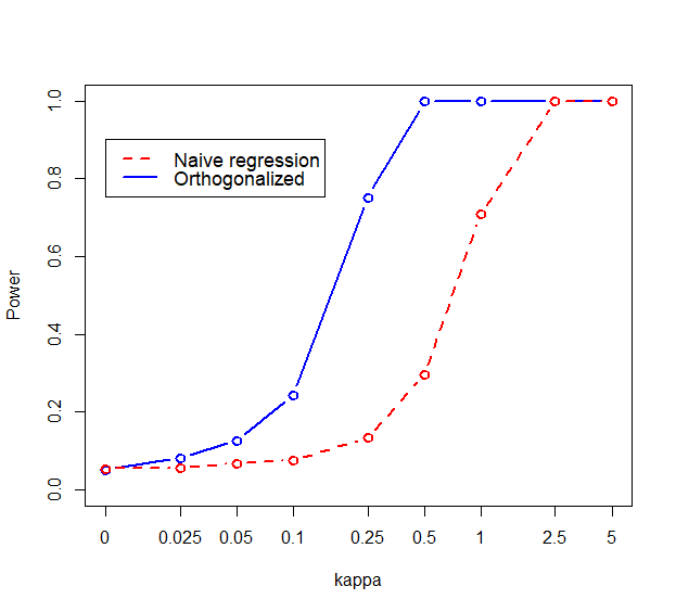
We illustrate how to apply orthogonalization to improve power in testing using variables in the ’mtcars’ dataset in R. In this popular example dataset [5] we regress gas mileage for different cars on the characteristics of their engine. This application was chosen specifically due to the high correlations among predictors (0.90). Selecting a couple of features, number of cylinders and displacement, we find the following relationship for consumption in miles per gallon by fitting the standard regression model: $\textit{mpg}=34.661-1.587\textit{cyl}-0.021\textit{disp}$, where the error standard deviation is $\sigma=3.055$. We now wish to see whether power improves when we orthogonalize the inputs, and, to check this, we will simulate $N=10,000$ replicated datasets, each of which keeps all of the same $n=32$ car models, but simulates random values for mpg based on the following model:

Notice that this matches the original data fit when $\kappa=1$, and we will vary $\kappa$ to achieve smaller or larger effect sizes, while keeping the relative effects of the predictors constant. We orthogonalize the inputs on number of cylinders first, and compare the power curve for testing coefficient of cyl against the power of the corresponding test from the original regression (the ”naive model”). Later, we will do the orthogonalization on disp first and test that parameter’s coefficient. When fitting both the naive and orthogonal models, we will center all variables first, including the response mpg, and we will fit without an intercept term. This is to avoid a highly significant linear combination of basis vectors that matches the intercept vector (i.e., the vector of ones), in the orthogonal model. We assume the signs of the coefficients in both the naive and orthogonalized models to be known, which makes it sensible to conduct one-sided tests. This assumption is realistic in practice, where analysts often know the directions of effects, at least for the most important features. The sign of $\Delta$ can be computed, if desired, to check whether a power boost can be expected by the orthogonal approach. To do this, multiply the regression equation by $-1$, which makes the outcome negative miles per gallon, and the coefficients $\beta_{cyl}=1.587\kappa$ and $\beta_{disp}=0.021\kappa$. Vector $\bm{q}_{1}$ (the first row of $Q^{-1}$) can be computed by following the formulas in the Appendix; thus, holding $cyl$ as the fixed direction, $\bm{q}_{1}=(0.10,-0.21)$. Using the coefficient values as in the data generating model, we get $\Delta=0.92\kappa>0$ which means that the test using the orthonormal regression will be more powerful.

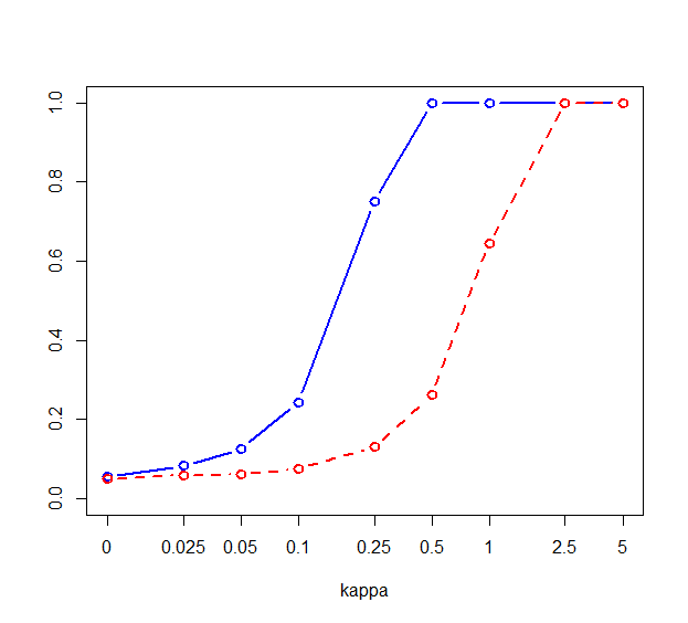
Figure 1 shows the power curves for both models, and for the two ways of orthogonalizing the features. Testing for the coefficient of the first feature $\bm{m}_{1}^{\perp}$ is visibly more powerful than testing for $\bm{m}_{1}$ in the naive model. The situation is almost identical when switching the order of cyl and disp, showing that the approach works regardless of which variable we choose as important.

There are some strong arguments for orthogonalizing highly correlated variables in regression. This paper has focused on the power advantage, and the knowledge that the coefficient tests are UMPU in this case. There are even more obvious advantages to this approach, still. One is that of eliminating collinearity without having to throwing away predictors, which loses potentially valuable information. Another advantage is that this approach does away with the need to include interaction terms. Indeed, with $p$ predictors there are potentially $p(p-1)/2$ interaction terms that can (or should) be considered, and many more three way interactions. With an orthogonal set of predictors, this is no longer the case as features are uncorrelated. This will significantly preserve power in inferences about the parameters.

The disadvantage of this approach, which has become apparent from discussions with statistical practitioners (consultants), is that of interpretability. Interpreting the remainder of one predictor after regressing on a few others may not be easy, and in many cases, this will not be desirable. For instance, health studies typically include demographic variables in analysis, such as age and sex, among others; these should probably be kept as such, for the sake of interpretability. We do not advocate that orthogonalization should be used routinely, and for all features. However, here are a few cases where it might be sensible to include this approach, at least for a subset of the feature space:

1. 1.

   With highly correlated variables that measure roughly the same thing. In socioeconomic studies, as an example, gross and net income are both measures of income and likely to be highly correlated. If it is meaningful to keep both, then the interpretation of the coefficient for each might be difficult, because if two predictors are close to collinear, then it is likely that the fit to data will result in a positive coefficient for one, and a negative coefficient for the other. Of course, this does not mean that gross and net income have opposite effects, rather, this is likely to be an artifact of multicollinearity. In this case, it makes more sense to decide on one predictor (e.g., gross income) to be interpreted as the main effect for income, and include the orthogonal component of net income as an extra effect due to, say, differential taxation of individuals that earn the same salary before tax.

2. 2.

   When there is a natural ordering in importance of predictors. For example, to an engineer looking at the fuel efficiency of different engines, it might be apparent that engine volume (displacement) is mainly what drives consumption, while number of cylinders might be simply a design choice that correlates with larger, more powerful engines. In this case, there would be a causal relationship between $disp$ and $mpg$, with $cyl$ being an intermediary variable of secondary importance that mediates the effect of $disp$. It would then make sense to orthogonalize on $disp$ as the main predictor, with the remainder term $cyl^{\perp\,disp}$ being the extra contribution of $cyl$ that is not related to engine size. This example spells out how an orthogonal remainder can be interpreted.

3. 3.

   In model building, since adding extra terms to the model does not change the estimated effects of previous predictors. As a follow-up to the previous point, when building a linear model through e.g., forward regression, one undesirable feature is that coefficients change every time a new term is added. This problem disappears when using orthogonalized predictors, as adding an extra dimension to the orthonormal basis does not change the projection of the data vector on the previous basis vectors. As such, parameters of full and reduced models will not lead to potentially contradictory interpretations.

Given all the advantages of orthogonalization, it is surprising that this approach has not gained more popularity in statistical practice.

RGR is based at the George & Fay Yee Centre for Healthcare Innovation. Support for CHI is provided by University of Manitoba, Canadian Institutes for Health Research, Province of Manitoba, and Shared Health Manitoba.

References

- [1] P.K. Bhattacharya and Prabir Burman. Hypothesis Testing. In Theory and Methods of Statistics, pages 125–177. Elsevier, 2016.
- [2] Sungsub Choi, W. J. Hall, and Anton Schick. Asymptotically uniformly most powerful tests in parametric and semiparametric models. The Annals of Statistics, 24(2), April 1996.
- [3] Merlise Clyde, Heather Desimone, and Giovanni Parmigiani. Prediction Via Orthogonalized Model Mixing. 2024.
- [4] Michele Forina, Silvia Lanteri, Monica Casale, and M. Conception Cerrato Oliveros. Stepwise orthogonalization of predictors in classification and regression techniques: An “old” technique revisited. Chemometrics and Intelligent Laboratory Systems, 87(2):252–261, June 2007.
- [5] Harold V. Henderson and Paul F. Velleman. Building Multiple Regression Models Interactively. Biometrics, 37(2):391, June 1981.
- [6] Maxwell L. King and Murray D. Smith. Joint one-sided tests of linear regression coefficients. Journal of Econometrics, 32(3):367–383, August 1986.
- [7] Erich L. Lehmann and Joseph P. Romano. Testing statistical hypotheses. Springer texts in statistics. Springer, New York, 3. ed., correct. at 4. print edition, 2008.
- [8] Xiaochang Lin, Jiewen Guan, Bilian Chen, and Yifeng Zeng. Unsupervised Feature Selection via Orthogonal Basis Clustering and Local Structure Preserving. IEEE Transactions on Neural Networks and Learning Systems, 33(11):6881–6892, November 2022.
- [9] Milan Randić. Mathematical chemistry illustrations: a personal view of less known results. Journal of Mathematical Chemistry, 57(1):280–314, January 2019.
- [10] Milan Šoškić, Dejan Plavšić, and Nenad Trinajstić. Link between Orthogonal and Standard Multiple Linear Regression Models. Journal of Chemical Information and Computer Sciences, 36(4):829–832, January 1996. Publisher: American Chemical Society.
Appendix
Going through the orthogonalization steps, we obtain the following new basis in closed form for up to three predictors