A uniqueness theorem for higher order anharmonic oscillators

Søren Fournais and Mikael Persson Sundqvist Aarhus University, Department of Mathematics, Ny Munkegade 181, 8000 Aarhus C, Denmark fournais@imf.au.dk Lund University, Department of Mathematical Sciences, Lund, Sweden mickep@maths.lth.se

Abstract.

We study for $\alpha\in\mathbb{R}$ , $k\in{\mathbb{N}}\setminus\{0\}$ the family of self-adjoint operators

-\frac{d^{2}}{dt^{2}}+\Bigl{(}\frac{t^{k+1}}{k+1}-\alpha\Bigr{)}^{2}

in $L^{2}(\mathbb{R})$ and show that if $k$ is even then $\alpha=0$ gives the unique minimum of the lowest eigenvalue of this family of operators. Combined with earlier results this gives that for any $k\geq 1$ , the lowest eigenvalue has a unique minimum as a function of $\alpha$ .

Key words and phrases:

Eigenvalue estimation, Anharmonic oscillator, Spectral parameter.

1991 Mathematics Subject Classification:

47A75; 47E05, 34L15, 34B08

1. Introduction

1.1. Definition of $\mathfrak{Q}^{(k)}(\alpha)$ and main result

For any $k\in{\mathbb{N}}\setminus\{0\}$ and $\alpha\in\mathbb{R}$ we define the operator

\mathfrak{Q}^{(k)}(\alpha)=-\frac{d^{2}}{dt^{2}}+\Bigl{(}\frac{t^{k+1}}{k+1}-\alpha\Bigr{)}^{2},

as a self-adjoint operator in $L^{2}({\mathbb{R}})$ . This family of operators is connected with the study of Schrödinger operators with a magnetic field vanishing along a curve and with the Ginzburg-Landau theory of superconductivity. It first appeared in [9] (for $k=1$ ) and was later studied in [7, 10, 6, 5, 8, 2, 3, 4].

We denote by $\bigl{\{}\lambda_{j,\mathfrak{Q}^{(k)}(\alpha)}\bigr{\}}_{j=1}^{\infty}$ the increasing sequence of eigenvalues of $\mathfrak{Q}^{(k)}(\alpha)$ . In particular, $\lambda_{1,\mathfrak{Q}^{(k)}(\alpha)}$ is the ground state eigenvalue, and we denote by $u_{\alpha}$ the associated positive, $L^{2}$ -normalized eigenfunction.

The main result of the present paper is the following theorem.

Theorem 1.1.

Assume that $k\geq 2$ is an even integer. Then $\lambda_{1,\mathfrak{Q}^{(k)}(\alpha)}$ attains a unique minimum at $\alpha=0$ . Moreover, this minimum is non-degenerate.

Remark 1.2.

This extends the previous results and discussions in [5, 8], where similar results were obtained for odd $k$ . The non-degeneracy was proved in [8]. In that paper it was also shown that Theorem 1.1 is valid for large even $k$ . The fact that the minimum is attained at $\alpha=0$ was suggested by numerical computations done by V. Bonnaillie–Noël.

Combining our Theorem 1.1 with the results of [5, 8] we get the following complete answer.

Theorem 1.3.

For any $k\in{\mathbb{N}}\setminus\{0\}$ , the function $\alpha\mapsto\lambda_{1,\mathfrak{Q}^{(k)}(\alpha)}$ attains a unique minimum. Moreover, this minimum is non-degenerate.

The paper is organized as follows. In Section 2 we give several spectral bounds on the first two eigenvalues of $\mathfrak{Q}^{(k)}(\alpha)$ . These estimates are used to prove Theorem 1.1 for $2\leq k\leq 68$ in Section 3 and for $k\geq 70$ in Section 4.

2. Auxiliary results

2.1. Introduction

In this section we collect several spectral bounds that will help us in proving Theorem 1.1. In the following, we assume that $k$ denotes a positive even integer.

With the scaling $s=\alpha^{-1/(k+1)}t$ it becomes clear that the form domain of $\mathfrak{Q}^{(k)}(\alpha)$ is independent of $\alpha$ . Thus, we are allowed to use the machinery of analytic perturbation theory.

First we note that $\mathfrak{Q}^{(k)}(\alpha)$ and $\mathfrak{Q}^{(k)}(-\alpha)$ are unitarily equivalent (map $t\mapsto-t$ along with $\alpha\mapsto-\alpha$ ). This implies that the function $\alpha\mapsto\lambda_{1,\mathfrak{Q}^{(k)}(\alpha)}$ is even, and hence has a critical point at $\alpha=0$ . It is proved in [8] that this critical point is a nondegenerate minimum. This also follows from our estimates below.

Lemma 2.1.

If $\alpha_{c}$ is a critical point of $\lambda_{1,\mathfrak{Q}^{(k)}(\alpha)}$ , then

\int_{-\infty}^{+\infty}\Bigl{(}\frac{t^{k+1}}{k+1}-\alpha_{c}\Bigr{)}u_{\alpha_{c}}(t)^{2}\,dt=0

and

\int_{-\infty}^{+\infty}\Bigl{(}\frac{t^{k+1}}{k+1}-\alpha_{c}\Bigr{)}^{2}u_{\alpha_{c}}(t)^{2}\,dt=\frac{\lambda_{1,\mathfrak{Q}^{(k)}(\alpha_{c})}}{k+2}.

Sketch of proof.

The first identity, usually referred to as the Feynman–Hellmann formula, follows from first order perturbation theory,

\frac{\partial}{\partial\alpha}\lambda_{1,\mathfrak{Q}^{(k)}(\alpha)}=-2\int_{-\infty}^{+\infty}\Bigl{(}\frac{t^{k+1}}{k+1}-\alpha\Bigr{)}u_{\alpha}(t)^{2}\,dt.

The second is a virial type identity and is proved by scaling. We refer to [8] for the details. ∎

2.2. Positive second derivative

A key element in our approach is the following Lemma 2.2, which can be used to rule out local maxima under appropriate estimates on the first eigenvalues.

Lemma 2.2 (Lemma 2.3 in [8]).

If $\alpha_{c}$ is a critical point of $\lambda_{1,\mathfrak{Q}^{(k)}(\alpha)}$ and

\frac{k+2}{k+6}\lambda_{2,\mathfrak{Q}^{(k)}(\alpha_{c})}>\lambda_{1,\mathfrak{Q}^{(k)}(\alpha_{c})}

then

\frac{\partial^{2}}{\partial\alpha^{2}}\lambda_{1,\mathfrak{Q}^{(k)}(\alpha)}\Big{|}_{\alpha=\alpha_{c}}>0.

We give a sketch of the proof for the sake of completeness.

Sketch of proof.

The proof is based on perturbation theory. The second derivative of $\lambda_{1,\mathfrak{Q}^{(k)}(\alpha)}$ is given by

\frac{\partial^{2}}{\partial\alpha^{2}}\lambda_{1,\mathfrak{Q}^{(k)}(\alpha)}=2-4\int_{-\infty}^{+\infty}\Bigl{(}\frac{t^{k+1}}{k+1}-\alpha\Bigr{)}u_{\alpha}\bigl{(}\partial_{\alpha}u_{\alpha}\bigr{)}\,dt.

Here

\partial_{\alpha}u_{\alpha}=-2(\mathfrak{Q}^{(k)}(\alpha)-\lambda_{1,\mathfrak{Q}^{(k)}(\alpha)})^{-1}\Bigl{(}\frac{t^{k+1}}{k+1}-\alpha\Bigr{)}u_{\alpha},

where the inverse is the regularized resolvent. The rest of the proof uses Lemma 2.1, the bound

\|(\mathfrak{Q}^{(k)}(\alpha_{c})-\lambda_{1,\mathfrak{Q}^{(k)}(\alpha_{c})})^{-1}\|\leq(\lambda_{2,\mathfrak{Q}^{(k)}(\alpha_{c})}-\lambda_{1,\mathfrak{Q}^{(k)}(\alpha_{c})})^{-1},

and the Cauchy-Schwarz inequality. ∎

To apply Lemma 2.2 we need good upper bounds on $\lambda_{1,\mathfrak{Q}^{(k)}(\alpha)}$ and lower bounds on $\lambda_{2,\mathfrak{Q}^{(k)}(\alpha)}$ . These will be presented in the sections below.

2.3. Upper bounds

We will at several points need upper bounds on the first eigenvalue of $\mathfrak{Q}^{(k)}(\alpha)$ . They are given in this section.

Lemma 2.3.

Assume that $\alpha_{c}$ is a critical point of $\alpha\mapsto\lambda_{1,\mathfrak{Q}^{(k)}(\alpha)}$ . Then, for all $\alpha\in\mathbb{R}$ it holds that

\lambda_{1,\mathfrak{Q}^{(k)}(\alpha)}\leq\lambda_{1,\mathfrak{Q}^{(k)}(\alpha_{c})}+(\alpha-\alpha_{c})^{2}.

Proof.

This follows by inserting the eigenfunction $u_{\alpha_{c}}$ corresponding to $\lambda_{1,\mathfrak{Q}^{(k)}(\alpha_{c})}$ of $\mathfrak{Q}^{(k)}(\alpha_{c})$ into the quadratic form corresponding to $\mathfrak{Q}^{(k)}(\alpha)$ and using Lemma 2.1 ∎

Lemma 2.4.

For all $\alpha\geq 0$ it holds that

\lambda_{1,\mathfrak{Q}^{(k)}(\alpha)}\leq\alpha^{2}+A_{k},

with

A_{k}=\begin{cases}\frac{2^{3/2}}{9}\bigl{(}\frac{4\pi^{6}-210\pi^{4}+4410\pi^{2}-26775}{7}\bigr{)}^{1/4},&k=2,\\ \frac{\pi^{2}}{4}\frac{k+2}{k+1}\bigl{(}\frac{1}{4}(k+1)(2k+3)(2k+4)(2k+5)\bigr{)}^{-1/(k+2)},&k\geq 2.\\ \end{cases}

Proof.

For $k\geq 4$ we refer to Lemma 3.1 in [8]. For $k=2$ we use the same idea but with a different trial state. A calculation of the energy of the function

u(t)=\begin{cases}\frac{2}{\sqrt{3\rho}}\cos^{2}\bigl{(}\frac{\pi t}{2\rho}\bigr{)},&|t|<\rho,\\ 0,&|t|\geq\rho,\\ \end{cases}

gives ( $\|u\|=1$ )

	$\displaystyle\lambda_{1,\mathfrak{Q}^{(2)}(\alpha)}$	$\displaystyle\leq\int_{-\infty}^{+\infty}\|u^{\prime}(t)\|^{2}+\Bigl{(}\frac{t^{3}}{3}-\alpha\Bigr{)}^{2}\|u(t)\|^{2}\,dt$
		$\displaystyle=\alpha^{2}+\frac{\pi^{2}}{3\rho^{2}}+\frac{4\pi^{6}-210\pi^{4}+4410\pi^{2}-26775}{252\pi^{6}}\rho^{6}.$

Minimizing in $\rho$ , we get the bound

\lambda_{1,\mathfrak{Q}^{(2)}(\alpha)}\leq\alpha^{2}+\frac{2^{3/2}}{9}\Bigl{(}\frac{4\pi^{6}-210\pi^{4}+4410\pi^{2}-26775}{7}\Bigr{)}^{1/4}\leq\alpha^{2}+0.6642,

attained for

\rho=2^{1/4}\pi\Bigl{(}\frac{4\pi^{6}-210\pi^{4}+4410\pi^{2}-26775}{7}\Bigr{)}^{-1/8}\approx 2.57.

∎

The upper bound given in Lemma 2.4 is graphed (for $\alpha=0$ and $2\leq k\leq 70$ ) in Figure 1 on page 1.

Lemma 2.5.

The function

k\mapsto\frac{\pi^{2}}{4}\frac{k+2}{k+1}\Bigl{(}\frac{1}{4}(k+1)(2k+3)(2k+4)(2k+5)\Bigr{)}^{-1/(k+2)}

appearing in Lemma 2.4 is increasing for $k\geq 2$ . In particular it is always bounded from above by $\pi^{2}/4$ .

Proof.

We will in the proof consider $k$ to be a real variable. Taking the logarithmic derivative of the expression, we get

\frac{a_{3}k^{3}+a_{2}k^{2}+a_{1}k+a_{0}}{(k+1)(k+2)^{2}(2k+3)(2k+5)}

with (here we note that each term is increasing with $k$ and thus estimate from below with $k=2$ )

	$\displaystyle a_{3}$	$\displaystyle=4\log(2(k+1)(k+2)(2k+3)(2k+5))-0-8\log 2$
		$\displaystyle\geq 4\log 78-0\geq 73,$
	$\displaystyle a_{2}$	$\displaystyle=0\log(2(k+1)(k+2)(2k+3)(2k+5))-08-0\log 2$
		$\displaystyle\geq 0\log 78-08\geq 069,$
	$\displaystyle a_{1}$	$\displaystyle=1\log(2(k+1)(k+2)(2k+3)(2k+5))-89-2\log 2$
		$\displaystyle\geq 1\log 78-89\geq-02,$
	$\displaystyle a_{0}$	$\displaystyle=5\log(2(k+1)(k+2)(2k+3)(2k+5))-07-0\log 2$
		$\displaystyle\geq 5\log 78-07\geq-798.$

Now, the polynomial

p(k)=3.73k^{3}+10.69k^{2}-5.02k-17.98

satisfies

p(2)\approx 44.58\quad\text{and}\quad p^{\prime}(k)=11.19k^{2}+21.38k-5.02.

Since $p^{\prime}(k)>0$ for $k\geq 2$ we find that $p$ is positive for $k\geq 2$ . This implies that the function in the statement is increasing. The final part follows since the limit as $k\to+\infty$ is $\pi^{2}/4$ . ∎

2.4. Lower bounds

To be able to use Lemma 2.2 we need lower bounds on the second eigenvalue. The following function will appear in the bounds.

Lemma 2.6.

It holds that

	$\displaystyle h(a)$	$\displaystyle=\max_{0<\sigma<1}(1-\sigma^{2})^{a/(a+2)}\sigma^{2/(a+2)}(a/2)^{4/(a+2)}$		(2.1)
		$\displaystyle=2^{-4/(a+2)}a^{(a+4)/(a+2)}(a+1)^{1/(a+2)-1}.$		(2.1)

Moreover, $\lim_{a\to+\infty}h(a)=1$ .

Proof.

Differentiating $(1-\sigma^{2})^{a/(a+2)}\sigma^{2/(a+2)}(a/2)^{4/(a+2)}$ with respect to $\sigma$ gives

\frac{2^{(a-2)/(a+2)}a^{4/(a+2)}\sigma^{-a/(a+2)}\bigl{(}1-\sigma^{2}\bigr{)}^{-2/(a+2)}\bigl{(}1-(a+1)\sigma^{2}\bigr{)}}{a+2},

with the unique zero (in $0<\sigma<1$ ) at $\sigma=1/\sqrt{a+1}$ . Since the function is zero at the endpoints and positive for $0<\sigma<1$ this must be the maximum. This proves (2.1)

The rest follows by a simple analysis of the right hand side of (2.1). The derivative equals

h^{\prime}(a)=\frac{2^{-4/(a+2)}a^{2/(a+2)}(a+1)^{1/(a+2)-1}\bigl{[}a\bigl{(}4+4\log 2-2\log a-\log(a+1)\bigr{)}+8\bigr{]}}{(a+2)^{2}}.

∎

Lemma 2.7.

For all real $\alpha$ and all even $k\geq 2$ it holds that

\mathfrak{Q}^{(k)}(\alpha)\geq h(k)\biggl{[}-\frac{d^{2}}{dt^{2}}+\Bigl{(}\frac{t^{k/2}}{k/2}\Bigr{)}^{2}\biggr{]},

where $h$ is the function from Lemma 2.6.

Proof.

Let $\mathfrak{A}=-i\frac{d}{dt}$ and $\mathfrak{B}=\bigl{(}\frac{t^{k+1}}{k+1}-\alpha\bigr{)}$ . Then the commutator $[\mathfrak{A},\mathfrak{B}]$ equals

[\mathfrak{A},\mathfrak{B}]=-it^{k}.

With the Cauchy–Schwarz inequality and the weighted arithmetic-geometric mean inequality, we find that (for all $0<\sigma<1$ )

\mathfrak{Q}^{(k)}(\alpha)\geq-(1-\sigma^{2})\frac{d^{2}}{dt^{2}}+\sigma t^{k}=-(1-\sigma^{2})\frac{d^{2}}{dt^{2}}+\sigma(k/2)^{2}\Bigl{(}\frac{t^{k/2}}{k/2}\Bigr{)}^{2}.

Scaling the variable and invoking Lemma 2.6 gives the result. ∎

Lemma 2.8.

Let $h$ be the function in Lemma 2.6. For all real $\alpha$ and all even $k\geq 2$ it holds that

\lambda_{2,\mathfrak{Q}^{(k)}(\alpha)}\geq B_{k},

with

B_{k}=h(k)\frac{3^{2k/(k+2)}(k+2)}{2^{(2k-2)/(k+2)}k^{(k+4)/(k+2)}}=\frac{3^{\frac{2k}{k+2}}(k+2)}{2^{\frac{2k+2}{k+2}}(k+1)^{\frac{k+1}{k+2}}}.

Proof.

Let $T>0$ . We use the estimate

\Bigl{(}\frac{t^{k/2}}{k/2}\Bigr{)}^{2}\geq\frac{2}{k}T^{k-2}t^{2}-\frac{2k-4}{k^{2}}T^{k},

valid for all $t\in\mathbb{R}$ . Comparing with the harmonic oscillator, and using Lemma 2.7, we get the required estimate for the second eigenvalue. The optimal choice of $T$ is

T=\Bigl{(}\frac{3\sqrt{2k}}{4}\Bigr{)}^{2/(k+2)}.

(2.2)

∎

The lower bound of $\lambda_{2,\mathfrak{Q}^{(k)}(\alpha)}$ in Lemma 2.8 will tend to $9/4$ as $k\to+\infty$ , which compared to the limit $\pi^{2}/4$ for the first eigenvalue is not good enough. Our next aim is to improve this lower bound on $\lambda_{2,\mathfrak{Q}^{(k)}(\alpha)}$ for large $k$ .

Lemma 2.9.

Assume that $k\geq 70$ is even and $\alpha\in\mathbb{R}$ . Then

\lambda_{2,\mathfrak{Q}^{(k)}(\alpha)}\geq\widetilde{B}_{k},

with

\widetilde{B}_{k}=\frac{\sqrt{5}-1}{2}\Biggl{(}\frac{\pi-\arctan\Bigl{(}\sqrt{\frac{(\pi/1.1)^{2}}{1.1^{70}-(\pi/1.1)^{2}}}\Bigr{)}}{1.1}\Biggr{)}^{2}\geq 4.719.

Proof.

We first do the commutator estimate

\mathfrak{Q}^{(k)}(\alpha)\geq-(1-\sigma^{2})\frac{d^{2}}{dt^{2}}+\sigma t^{k}=\frac{\sqrt{5}-1}{2}\Bigl{(}-\frac{d^{2}}{dt^{2}}+t^{k}\Bigr{)},

where $\sigma$ in the latter step is chosen to be $\frac{\sqrt{5}-1}{2}$ . Next we note that the second eigenvalue of

-\frac{d^{2}}{dt^{2}}+t^{k}

in $L^{2}(\mathbb{R})$ equals the first eigenvalue of the operator

-\frac{d^{2}}{dt^{2}}+t^{k}

in $L^{2}(\mathbb{R}^{+})$ with Dirichlet condition at $t=0$ . Let $T>1$ . Then

-\frac{d^{2}}{dt^{2}}+t^{k}\geq\mathfrak{D}^{(k)}:=-\frac{d^{2}}{dt^{2}}+T^{k}\chi_{\{t>T\}},

where we, again, impose a Dirichlet condition at $t=0$ . Here $\chi_{D}$ denotes the characteristic function of the set $D$ . Let us estimate the first eigenvalue $\lambda_{1,\mathfrak{D}^{(k)}}$ of $\mathfrak{D}^{(k)}$ . Clearly

\lambda_{1,\mathfrak{D}^{(k)}}\leq\Bigl{(}\frac{\pi}{T}\Bigr{)}^{2},

which is what one gets considering $(0,T)$ and imposing a Dirichlet condition at $t=T$ . The ground state of $\mathfrak{D}^{(k)}$ is given by (in the rest of this proof we write $\lambda=\lambda_{1,\mathfrak{D}^{(k)}}$ )

u(t)=\begin{cases}c_{1}\sin(\sqrt{\lambda}t),&0\leq t\leq T,\\ c_{2}e^{-\omega t},&t\geq T,\end{cases}

where

-\omega^{2}+T^{k}=\lambda

and where we have the gluing conditions at $t=T$ :

	$\displaystyle c_{1}\sin(\sqrt{\lambda}T)$	$\displaystyle=c_{2}e^{-\omega T}\quad\text{and}$
	$\displaystyle c_{1}\sqrt{\lambda}\cos(\sqrt{\lambda}T)$	$\displaystyle=-c_{2}\omega e^{-\omega T}.$

This gives the equation (in $\sqrt{\lambda}$ )

\tan(\sqrt{\lambda}T)=-\frac{\sqrt{\lambda}}{\omega}\quad\text{i.e.}\quad\tan(\pi-\sqrt{\lambda}T)=\frac{\sqrt{\lambda}}{\omega},

which has a unique solution in the interval $\frac{\pi}{2T}<\sqrt{\lambda}<\frac{\pi}{T}$ . We think of $T>1$ and $k$ large, so that $\sqrt{\lambda}/\omega$ is small, and get

\frac{\sqrt{\lambda}}{\omega}=\sqrt{\frac{\lambda}{T^{k}-\lambda}}\leq\sqrt{\frac{(\pi/T)^{2}}{T^{k}-(\pi/T)^{2}}}.

And so by monotonicity

\pi-\sqrt{\lambda}T\leq\arctan\biggl{(}\sqrt{\frac{(\pi/T)^{2}}{T^{k}-(\pi/T)^{2}}}\biggr{)},

i.e.

\lambda\geq\Biggl{(}\frac{\pi-\arctan\Bigl{(}\sqrt{\frac{(\pi/T)^{2}}{T^{k}-(\pi/T)^{2}}}\Bigr{)}}{T}\Biggr{)}^{2}.

Now, without optimizing, we find that with $T=1.1$ and $k\geq 70$ it holds that

\lambda_{2,\mathfrak{Q}^{(k)}(\alpha)}\geq\frac{\sqrt{5}-1}{2}\lambda\geq\frac{\sqrt{5}-1}{2}\Biggl{(}\frac{\pi-\arctan\Bigl{(}\sqrt{\frac{(\pi/1.1)^{2}}{1.1^{70}-(\pi/1.1)^{2}}}\Bigr{)}}{1.1}\Biggr{)}^{2}\geq 4.719.

∎

We will also need lower bounds on $\lambda_{1,\mathfrak{Q}^{(k)}(\alpha)}$ for large $\alpha$ . This is the content of the following two Lemmas.

Lemma 2.10.

For $\alpha\geq 3/2$ and even $k\geq 2$ it holds that

\lambda_{1,\mathfrak{Q}^{(k)}(\alpha)}\geq C_{k},

(2.3)

with

C_{k}=\min\Biggl{(}\Bigl{(}\frac{3}{2}-\frac{1}{k+1}\Bigr{)}^{2},\frac{\frac{3}{2}(k+1)-1}{(k+1)\bigl{(}\bigl{(}\frac{3}{2}(k+1)\bigr{)}^{1/(k+1)}-1\bigr{)}}\Theta_{0}\Biggr{)}.

In particular, if $2\leq k\leq 68$ it holds that

\lambda_{1,\mathfrak{Q}^{(k)}(\alpha)}>\lambda_{1,\mathfrak{Q}^{(k)}(0)}

for all $\alpha\geq 3/2$ .

Proof.

First we note that the potential $\bigl{(}\frac{t^{k+1}}{k+1}-\alpha\bigr{)}^{2}$ is decreasing for all $t<1$ (in fact for all $t<((k+1)\alpha)^{1/(k+1)}$ ), and thus it is greater than $(1/(k+1)-3/2)^{2}$ for all $t<1$ and all $\alpha\geq 3/2$ .

For $t\geq 1$ and $\alpha\geq 3/2$ , we estimate

	$\displaystyle\Bigl{(}\frac{t^{k+1}}{k+1}-\alpha\Bigr{)}^{2}$	$\displaystyle=\frac{1}{(k+1)^{2}}\Biggl{(}\sum_{j=0}^{k}t^{k-j}\bigl{(}\alpha(k+1)\bigr{)}^{1/(k+1)}\Biggr{)}^{2}\Bigl{(}t-\bigl{(}\alpha(k+1)\bigr{)}^{1/(k+1)}\Bigr{)}^{2}$
		$\displaystyle\geq\frac{1}{(k+1)^{2}}\biggl{(}\frac{\frac{3}{2}(k+1)-1}{\bigl{(}\frac{3}{2}(k+1)\bigr{)}^{1/(k+1)}-1}\biggr{)}^{2}\Bigl{(}t-\bigl{(}\alpha(k+1)\bigr{)}^{1/(k+1)}\Bigr{)}^{2}.$

Here we used that the expression in the big sum is increasing both in $t$ and in $\alpha$ , and then applied the formula for a geometric sum.

Thus, comparing with the minimum of the potential for $t<1$ and with the de Gennes operator for $t\geq 1$ we conclude (2.3).

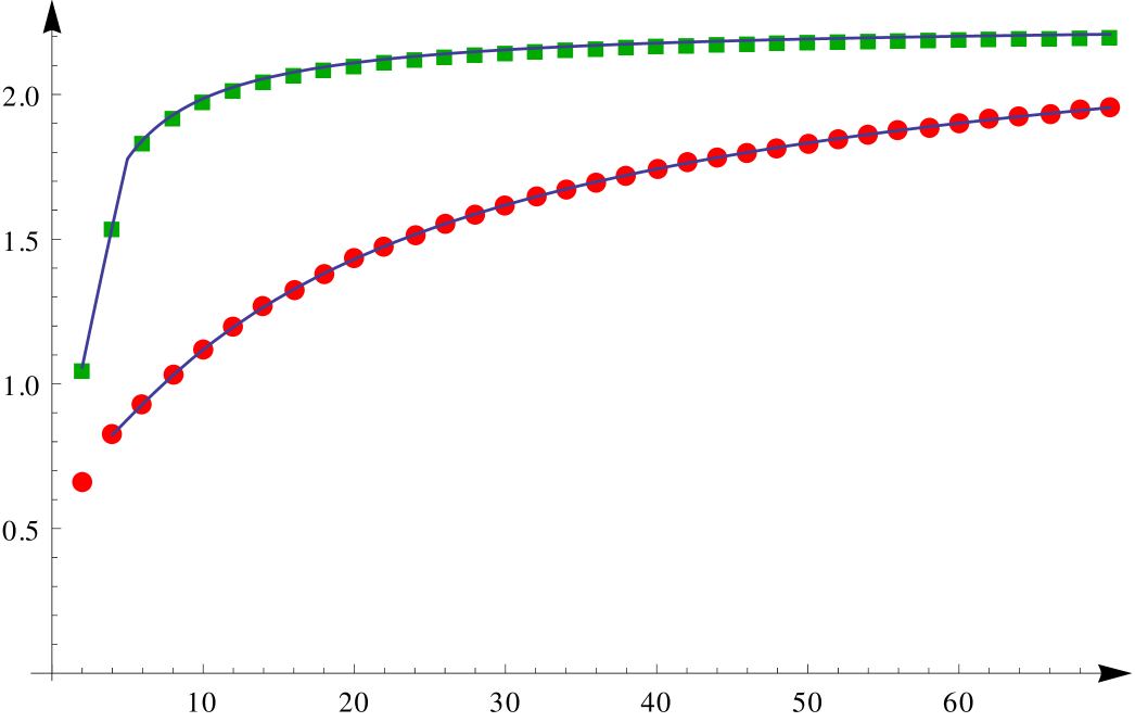
The last part follows by comparing the upper bound in Lemma 2.4 with the just obtained lower bound (and using the fact that $\Theta_{0}>0.59$ which is known from [1]). This is done in Figure 1.

Refer to caption — Figure 1. The disks are the upper bounds on $\lambda_{1,\mathfrak{Q}^{(k)}(0)}$ from Lemma 2.4 as a function of $k$ . The squares are the lower bounds on $\lambda_{1,\mathfrak{Q}^{(k)}(\alpha)}$ , $\alpha\geq 3/2$ , as a function of $k$ , from Lemma 2.10.

∎

We need a better bound for large $k$ than the one given in Lemma 2.10. We use instead $\alpha=2.8$ as lower bound and find that

Lemma 2.11.

For $\alpha\geq 2.8$ it holds that

\lambda_{1,\mathfrak{Q}^{(k)}(\alpha)}\geq\min\Biggl{(}\Bigl{(}2.8-\frac{1}{k+1}\Bigr{)}^{2},\frac{2.8(k+1)-1}{(k+1)\bigl{(}\bigl{(}2.8(k+1)\bigr{)}^{1/(k+1)}-1\bigr{)}}\Theta_{0}\Biggr{)}.

For $k\geq 70$ the first term is the smallest one, i.e.

\lambda_{1,\mathfrak{Q}^{(k)}(\alpha)}\geq\Bigl{(}2.8-\frac{1}{k+1}\Bigr{)}^{2}\geq\Bigl{(}2.8-\frac{1}{71}\Bigr{)}^{2}\geq 7.76.

In particular $\lambda_{1,\mathfrak{Q}^{(k)}(\alpha)}$ cannot obtain its global minimum for $\alpha\geq 2.8$ .

Proof.

The proof is exactly the same as the proof of Lemma 2.10. The second statement follows from noticing that the second term in the minimum is increasing and that its value at $k=70$ is

\frac{2.8(70+1)-1}{(70+1)\bigl{(}\bigl{(}2.8(70+1)\bigr{)}^{1/(70+1)}-1\bigr{)}}\Theta_{0}\geq 21.2,

while the first term in the minimum is less than $2.8^{2}=7.84$ .

The last statement follows by using Lemma 2.5 to conclude that the upper bound on $\lambda_{1,\mathfrak{Q}^{(k)}(0)}$ in Lemma 2.4 is less than $\pi^{2}/4$ for all $k$ . Since $\pi^{2}/4$ is less than $7.76$ we are done. ∎

3. Proof of Theorem 1.1 for $2\leq k\leq 68$

Lemma 3.1.

For each even $k$ , $2\leq k\leq 68$ , let

\alpha^{*}=\sqrt{\frac{k+2}{k+6}B_{k}-A_{k}},

where $A_{k}$ is the upper bound on $\lambda_{1,\mathfrak{Q}^{(k)}(0)}$ from Lemma 2.4 and $B_{k}$ is the lower bound on $\lambda_{2,\mathfrak{Q}^{(k)}(\alpha)}$ from Lemma 2.8. Then, $\alpha\mapsto\lambda_{1,\mathfrak{Q}^{(k)}(\alpha)}$ has no critical point in the interval $0<\alpha<\alpha^{*}$ .

Proof.

Assume, to get a contradiction, that $0<\alpha_{c}<\alpha^{*}$ is a critical point. Then, invoking Lemma 2.4 and the definition of $\alpha^{*}$ above, we find that

\lambda_{1,\mathfrak{Q}^{(k)}(\alpha_{c})}\leq A_{k}+\alpha_{c}^{2}<A_{k}+(\alpha^{*})^{2}=\frac{k+2}{k+6}B_{k}\leq\frac{k+2}{k+6}\lambda_{2,\mathfrak{Q}^{(k)}(\alpha_{c})},

which by Lemma 2.2 implies that $\alpha_{c}$ is a non-degenerate local minimum. Hence all critical points in $0<\alpha<\alpha^{*}$ must be non-degenerate local minimums. Now we know that zero is a non-degenerate local minimum. Since there cannot be more than one such in a row we get a contradiction. ∎

Lemma 3.2.

With $k$ and $\alpha^{*}$ as in the previous Lemma it holds that $\lambda_{1,\mathfrak{Q}^{(k)}(\alpha)}$ cannot attain its global minimal value in the interval $[\alpha^{*},2\alpha^{*})$ .

Proof.

Assume, to get a contradiction, that we have one $\alpha_{c}$ in this interval where we have have a global minimum. Then, in particular, $\lambda_{1,\mathfrak{Q}^{(k)}(\alpha_{c})}\leq\lambda_{1,\mathfrak{Q}^{(k)}(0)}$ . Thus, combining again Lemmas 2.2 and 2.3 we find that any critical point in $[\alpha^{*},\alpha_{c})$ must be a non-degenerate minimum. However, by the previous Lemma we know that there are no critical points in $(0,\alpha^{*})$ , and so again we would have two non-degenerate minimums in a row. Since that is not possible we get a contradiction. ∎

Lemma 3.3.

Assume that $2\leq k\leq 68$ is even. Denote by

\alpha^{**}=\frac{3}{2}-\sqrt{C_{k}-A_{k}},

where, again, $A_{k}$ is the upper bound on $\lambda_{1,\mathfrak{Q}^{(k)}(0)}$ from Lemma 2.4 and $C_{k}$ is the lower bound on $\lambda_{1,\mathfrak{Q}^{(k)}(\alpha)}$ from Lemma 2.10.

If $\alpha>\alpha^{**}$ then $\lambda_{1,\mathfrak{Q}^{(k)}(\alpha)}$ cannot attain its global minimum.

Proof.

First we note that if $\alpha\geq 3/2$ then $\lambda_{1,\mathfrak{Q}^{(k)}(\alpha)}\geq\lambda_{1,\mathfrak{Q}^{(k)}(0)}$ by Lemma 2.10. Assume, to get a contradiction, that $\lambda_{1,\mathfrak{Q}^{(k)}(\alpha)}$ attains its global minimum for a $\alpha^{**}<\alpha_{c}<3/2$ . Then, by Lemma 2.3 it holds that

	$\displaystyle\lambda_{1,\mathfrak{Q}^{(k)}(3/2)}$	$\displaystyle\leq\lambda_{1,\mathfrak{Q}^{(k)}(\alpha_{c})}+(\alpha_{c}-3/2)^{2}$
		$\displaystyle\leq\lambda_{1,\mathfrak{Q}^{(k)}(0)}+(\alpha^{**}-3/2)^{2}$
		$\displaystyle<A_{k}+C_{k}-A_{k}=C_{k}.$

But this contradicts Lemma 2.10. ∎

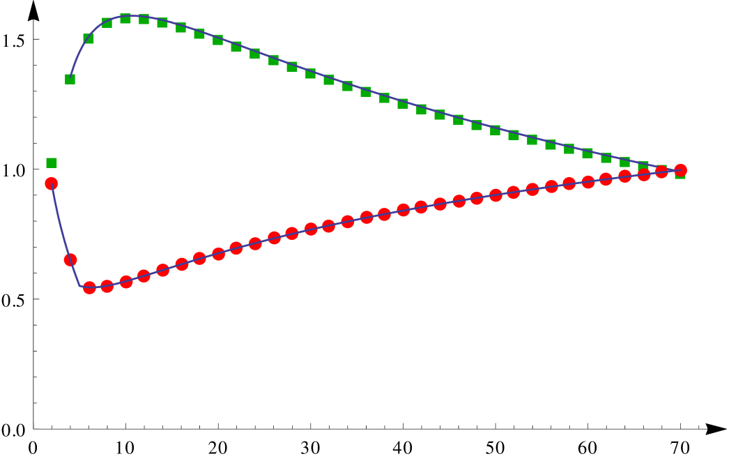
The proof of Theorem 1.1 is completed for $2\leq k\leq 68$ by ploting $2\alpha^{*}$ and $\alpha^{**}$ and noting that $2\alpha^{*}>\alpha^{**}$ for these $k$ . This is done in Figure 2.

4. Proof of Theorem 1.1 for $k\geq 70$

Lemma 4.1.

Assume that $k\geq 70$ . Then $\lambda_{1,\mathfrak{Q}^{(k)}(\alpha)}$ cannot have its global minimum for $0<\alpha<2.83$ .

Proof.

This follows the same lines as the proofs of Lemmas 3.1 and 3.2. We let

\alpha^{*}=\sqrt{\frac{k+2}{k+6}\widetilde{B}_{k}-A_{k}},

where $A_{k}$ is the upper bound on $\lambda_{1,\mathfrak{Q}^{(k)}(0)}$ from Lemma 2.4 (which is increasing in $k$ by Lemma 2.5) and $\widetilde{B}_{k}$ is the lower bound on $\lambda_{2,\mathfrak{Q}^{(k)}(\alpha)}$ from Lemma 2.9. For $k\geq 70$ we note that

2\alpha^{*}\geq 2\sqrt{\frac{72}{76}\times 4.719-\frac{\pi^{2}}{4}}\geq 2.83.

∎

Combining this result with Lemma 2.11 we find that $\lambda_{1,\mathfrak{Q}^{(k)}(\alpha)}$ cannot have its minimum attained for $\alpha>0$ . This proves Theorem 1.1.

Acknowledgements

SF was partially supported by the Lundbeck Foundation, the Danish Natural Science Research Council and the European Research Council under the European Community’s Seventh Framework Program (FP7/2007–2013)/ERC grant agreement 202859.

References

[1] V. Bonnaillie-Noël. Harmonic oscillators with Neumann condition of the half-line. Commun. Pure Appl. Anal., 11(6):2221–2237, 2012.
[2] N. Dombrowski and N. Raymond. Semiclassical analysis with vanishing magnetic fields.
[3] S. Fournais and M. Persson. Strong diamagnetism for the ball in three dimensions. Asymptot. Anal., 72(1-2):77–123, 2011.
[4] S. Fournais and M. Persson Sundqvist. Lack of diamagnetism and the Little–Parks effect. arXiv:XXXX:XXXX, 2013.
[5] B. Helffer. The Montgomery model revisited. Colloquium Mathematicum, volume in honor of A. Hulanicki, 118(2):391–400, 2010.
[6] B. Helffer and Y. A. Kordyukov. Spectral gaps for periodic Schrödinger operators with hypersurface magnetic wells. In Mathematical results in quantum mechanics, pages 137–154. World Sci. Publ., Hackensack, NJ, 2008.
[7] B. Helffer and A. Morame. Magnetic bottles in connection with superconductivity. J. Funct. Anal., 185(2):604–680, 2001.
[8] B. Helffer and M. Persson. Spectral properties of higher order anharmonic oscillators. Journal of Mathematical Sciences, 165(1), 2010.
[9] R. Montgomery. Hearing the zero locus of a magnetic field. Comm. Math. Phys., 168(3):651–675, 1995.
[10] X.-B. Pan and K.-H. Kwek. Schrödinger operators with non-degenerately vanishing magnetic fields in bounded domains. Trans. Amer. Math. Soc., 354(10):4201–4227 (electronic), 2002.

A uniqueness theorem for higher order anharmonic oscillators

Abstract.

Key words and phrases:

1991 Mathematics Subject Classification:

1. Introduction

1.1. Definition of 𝔔(k)​(α)\mathfrak{Q}^{(k)}(\alpha) and main result

Theorem 1.1.

Remark 1.2.

Theorem 1.3.

2. Auxiliary results

2.1. Introduction

Lemma 2.1.

Sketch of proof.

2.2. Positive second derivative

Lemma 2.2 (Lemma 2.3 in [8]).

Sketch of proof.

2.3. Upper bounds

Lemma 2.3.

Proof.

Lemma 2.4.

Proof.

Lemma 2.5.

Proof.

2.4. Lower bounds

Lemma 2.6.

Proof.

Lemma 2.7.

Proof.

Lemma 2.8.

Proof.

Lemma 2.9.

Proof.

Lemma 2.10.

Proof.

Lemma 2.11.

Proof.

3. Proof of Theorem 1.1 for 2≤k≤682\leq k\leq 68

Lemma 3.1.

Proof.

Lemma 3.2.

Proof.

Lemma 3.3.

Proof.

4. Proof of Theorem 1.1 for k≥70k\geq 70

Lemma 4.1.

Proof.

Acknowledgements

References

1.1. Definition of $\mathfrak{Q}^{(k)}(\alpha)$ and main result

3. Proof of Theorem 1.1 for $2\leq k\leq 68$

4. Proof of Theorem 1.1 for $k\geq 70$