A Variational Bayesian Inference-Inspired Unrolled Deep Network for MIMO Detection

Qian Wan, Jun Fang, , Yinsen Huang, Huiping Duan, and Hongbin Li Qian Wan, Jun Fang and Yinsen Huang are with the National Key Laboratory of Science and Technology on Communications, University of Electronic Science and Technology of China, Chengdu 611731, China, Email: JunFang@uestc.edu.cnHuiping Duan is with the School of Information and Communications Engineering, University of Electronic Science and Technology of China, Chengdu 611731, China, Email: huipingduan@uestc.edu.cnHongbin Li is with the Department of Electrical and Computer Engineering, Stevens Institute of Technology, Hoboken, NJ 07030, USA, E-mail: Hongbin.Li@stevens.eduThis work was supported in part by the National Science Foundation of China under Grants 61829103 and 61871421.©2022 IEEE. Personal use of this material is permitted. Permission from IEEE must be obtained for all other uses, in any current or future media, including reprinting/republishing this material for advertising or promotional purposes, creating new collective works, for resale or redistribution to servers or lists, or reuse of any copyrighted component of this work in other works.

Abstract

The great success of deep learning (DL) has inspired researchers to develop more accurate and efficient symbol detectors for multi-input multi-output (MIMO) systems. Existing DL-based MIMO detectors, however, suffer several drawbacks. To address these issues, in this paper, we develop a model-driven DL detector based on variational Bayesian inference. Specifically, the proposed unrolled DL architecture is inspired by an inverse-free variational Bayesian learning framework which circumvents matrix inversion via maximizing a relaxed evidence lower bound. Two networks are respectively developed for independent and identically distributed (i.i.d.) Gaussian channels and arbitrarily correlated channels. The proposed networks, referred to as VBINet, have only a few learnable parameters and thus can be efficiently trained with a moderate amount of training samples. The proposed VBINet-based detectors can work in both offline and online training modes. An important advantage of our proposed networks over state-of-the-art MIMO detection networks such as OAMPNet and MMNet is that the VBINet can automatically learn the noise variance from data, thus yielding a significant performance improvement over the OAMPNet and MMNet in the presence of noise variance uncertainty. Simulation results show that the proposed VBINet-based detectors achieve competitive performance for both i.i.d. Gaussian and realistic 3GPP MIMO channels.

Index Terms:

MIMO detection, variational Bayesian inference, unrolled deep networks.

I Introduction

Massive multiple-input multiple-output (MIMO) is a promising technology for next-generation wireless communication systems [1, 2, 3]. In massive MIMO systems, the base station (BS), equipped with tens or hundreds of antennas, simultaneously serves a smaller number of single-antenna users sharing the same time-frequency resource [4]. The large number of antennas at the BS helps achieve almost perfect inter-user interference cancelation and has the potential to enhance the spectrum efficiency by orders of magnitude. Nevertheless, large-scale MIMO poses a significant challenge for optimal signal detection. To realize the full potential of massive MIMO systems, it is of significance to develop advanced signal detection algorithms that can strike a good balance between performance and complexity [5].

Signal detection in the MIMO framework has been extensively investigated over the past decades. It is known that the maximum likelihood (ML) detector is an optimal detector but has a computational complexity that scales exponentially with the number of unknown variables. Linear detectors such as zero-forcing (ZF) and linear minimum mean-squared error (LMMSE) have a relatively low computational complexity, but they suffer a considerable performance degradation as compared with the ML detector. Recently, Bayesian inference or optimization-based iterative detectors, e.g. [6, 7, 8, 9, 10, 11], were proposed. Empirical results show that these iterative schemes such as the approximate message passing (AMP) and expectation propagation (EP)-based detectors can achieve excellent performance with moderate complexity [9, 10]. Nevertheless, the AMP-based or EP-based methods utilize a series of approximation techniques to facilitate the Bayesian inference. When the channel matrix has a small size or is ill-conditioned, the approximation may not hold valid, in which case these methods may suffer severe performance degradation.

More recently, the great success of deep learning (DL) in a variety of learning tasks has inspired researchers to use it as an effective tool to devise more accurate and efficient detection and estimation schemes [12, 13, 14, 15, 16, 17, 18]. The application of purely data-driven DL-based schemes, however, faces the challenges of a long training time as a result of the complicated network structure and a large number of learnable parameters [19, 20]. To address this issue, model-driven DL-based schemes were recently proposed for MIMO detection [21, 22, 23]. The main idea of model-driven DL detector is to unfold the iterative algorithm as a series of neural network layers with some learnable parameters. Specifically, DetNet seems to be one of the earliest works to study the problem of MIMO detection by unfolding the projected gradient descent algorithm [24]. The number of learnable parameters for DetNet, however, is still large. Thus it needs a large number of samples to train the neural network. As an extension of DetNet, WeSNet aims to reduce the model size by introducing a sparsity-inducing regularization constraint in conjunction with trainable weight-scaling functions [25]. In order to further reduce the number of learnable parameters of the network, OAMPNet, a neural architecture inspired by the orthogonal AMP algorithm, was proposed [22]. The OAMPNet has only four learnable parameters per layer, and thus is easy to train. Compared with DetNet, OAMPNet can achieve competitive performance with much fewer training samples. Both DetNet and OAMPNet are trained in an offline mode, i.e. they aim to learn a single detector during training for a family of channel matrices. Recently, another work [23] examined the MIMO detection problem from an online training perspective. The proposed MMNet can achieve a considerable performance improvement over OAMPNet when sufficient online training is allowed. Nevertheless, online training means that the model parameters are trained and tested for each realization of the channel. When the test channel sample is different from the training channel sample, MMNet would suffer a substantial amount of performance degradation. It should be noted that both OAMPNet and MMNet require the knowledge of the noise variance for symbol detection. In practice, however, the prior information about the noise variance is usually unavailable and inaccurate estimation may result in substantial performance loss.

Recently, the information bottleneck (IB) theory attracts much attention for providing an information theoretic view of deep learning networks [26, 27]. The IB approach has found applications in a variety of learning problems. It can also be applied to solve the MIMO detection problem. Consider extracting the relevant information that some signal $X$ provides about another one $Y$ that is of interest. IB formulates the problem of finding a representation $U$ that is maximally informative about $Y$ , while being minimally informative about $X$ [26]. Accordingly, the optimal mapping of the data $X$ to $U$ is found by solving a Lagrangian formulation. This problem can be solved by approximating its variational bound by parameterizing the encoder, decoder and prior distributions with deep neural networks. Nevertheless, when applied to MIMO detection, the IB approach needs a large number of learnable parameters. Therefore it still faces the challenge encountered by purely data-driven DL-based schemes.

In this paper, we propose a variational Bayesian inference-inspired unrolled deep network for MIMO detection. Our proposed deep learning architecture is mainly inspired by the inverse-free Bayesian learning framework [28], where a fast inverse-free variational Bayesian method was proposed via maximizing a relaxed evidence lower bound. Specifically, we develop two unrolled deep networks, one for i.i.d. Gaussian channels and the other for arbitrarily correlated channels. Our proposed networks, referred to as the variational Bayesian inference-inspired network (VBINet), have a very few learnable parameters and thus can be efficiently trained with a moderate number of training samples. The proposed VBINet can work in both offline and online training modes. An important advantage of our proposed networks over OAMPNet and MMNet is that the VBINet can automatically learn the noise variance from data, which is highly desirable in practical applications. In addition, the proposed VBINet has a low computational complexity, and each layer of the neural network only involves simple matrix-vector calculations. Simulation results show that the proposed VBINet-based detector achieves competitive performance for both i.i.d. Gaussian and 3GPP MIMO channels. Moreover, it attains a significant performance improvement over the OAMPNet and MMNet in the presence of noise variance uncertainty.

The rest paper is organized as follows. Section II discusses the MIMO detection problem. Section III provides a brief overviews of some state-of-the-art DL-based detectors. Section IV proposes an iterative detector for i.i.d. Gaussian channels within the inverse-free variational Bayesian framework. A deep network (VBINet) is then developed by unfolding the iterative detector in Section V. The iterative detector is extended to correlated channels in Section VI, and an improved VBINet is developed in Section VII for arbitrarily correlated channels. Numerical results are provided in Section VIII, followed by conclusion remarks in Section IX.

II Problem Formulation

We consider the problem of MIMO detection for uplink MIMO systems, in which a base station equipped with $N_{r}$ antennas receives signals from $N_{t}$ single-antenna users. The received signal vector $\boldsymbol{y}\in\mathbb{C}^{N_{r}}$ can be expressed as

\displaystyle\boldsymbol{y}=\boldsymbol{H}\boldsymbol{x}+\boldsymbol{n}

(1)

where $\boldsymbol{H}\in\mathbb{C}^{N_{r}\times N_{t}}$ denotes the MIMO channel matrix, and $\boldsymbol{n}\sim\mathcal{CN}(\boldsymbol{0},\frac{1}{\varepsilon}\boldsymbol{I})$ denotes the additive complex Gaussian noise. It is clear that the likelihood function of the received signal is given by

\displaystyle p(\boldsymbol{y}|\boldsymbol{x},\varepsilon)=\big{(}\frac{\varepsilon^{\frac{1}{2}}}{\sqrt{2\pi}}\big{)}^{N_{r}}\exp\left\{-\frac{\varepsilon\|\boldsymbol{y}-\boldsymbol{H}\boldsymbol{x}\|_{2}^{2}}{2}\right\}

(2)

where each element of the detected symbol $\boldsymbol{x}$ belongs to a discrete constellation set $\mathcal{C}=\{c_{1},\ldots,c_{M}\}$ . In other words, the prior distribution for $\boldsymbol{x}$ is given as

\displaystyle p(\boldsymbol{x})=\prod_{i=1}^{N_{t}}p(x_{i})

(3)

where

\displaystyle p(x_{i})=\sum_{j\in M}\frac{1}{M}\delta(x_{i}-c_{j})

(4)

in which $\delta(\cdot)$ stands for the Dirac delta function.

The optimal detector for (1) is the maximum-likelihood (ML) estimator formulated as follows [29, 23]

\displaystyle\min_{\boldsymbol{x}\in\mathcal{C}}\quad\|\boldsymbol{y}-\boldsymbol{H}\boldsymbol{x}\|_{2}^{2}

(5)

Although the ML estimator yields optimal performance, its computational complexity is prohibitively high. To address this difficulty, a plethora of detectors were proposed over the past few decades to strike a balance between complexity and detection performance. Recently, a new class of model-driven DL methods called algorithm unrolling or unfolding were proposed for MIMO detection. It was shown that model-driven DL-based detectors present a significant performance improvement over traditional iterative approaches. In the following, we first provide an overview of state-of-the-art model-driven DL-based detectors, namely, the OAMPNet [22] and the MMNET [23].

III Overview of State-Of-The-Art DL-Based Detectors

III-A OAMPNet

OAMPNet is a model-driven DL algorithm for MIMO detection, which is derived from the OAMP [30]. The advantage of OAMP over AMP is that it can be applied to unitarily-invariant matrices while AMP is only applicable to i.i.d Gaussian measurement matrices. OAMPNet can achieve better performance than OAMP, and can adapt to various channel environments by use of some learnable variables. Each iteration of the OAMPNet comprises the following two steps:

		$\displaystyle\text{LE}:\quad\quad\boldsymbol{r}_{t}=\boldsymbol{x}_{t}+\gamma_{t}\boldsymbol{W}_{t}(\boldsymbol{y}-\boldsymbol{H}\boldsymbol{x}_{t})$		(6)
		$\displaystyle\text{NLE}:\quad\boldsymbol{x}_{t+1}=\eta_{t}(\boldsymbol{r}_{t},\sigma_{t}^{2};\phi_{t},\xi_{t})$		(7)

where $\boldsymbol{x}_{t}$ denotes the current estimate of $\boldsymbol{x}$ , and $\boldsymbol{W}_{t}$ is given as [30]:

\displaystyle\boldsymbol{W}_{t}

\displaystyle=\frac{N_{t}}{\text{tr}\{\hat{\boldsymbol{W}}_{t}\boldsymbol{H}\}}\hat{\boldsymbol{W}}_{t}

(8)

in which $\hat{\boldsymbol{W}}_{t}$ is the LMMSE matrix, i.e.

\displaystyle\hat{\boldsymbol{W}}_{t}

\displaystyle=v_{t}^{2}\boldsymbol{H}^{H}(v_{t}^{2}\boldsymbol{H}\boldsymbol{H}^{H}+\boldsymbol{R}_{n})^{-1}

(9)

$v_{t}^{2}$ is the error variance of $\boldsymbol{x}_{t}-\boldsymbol{x}$ , and can be calculated as

	$\displaystyle v_{t}^{2}$	$\displaystyle=\text{Tr}\Big{\{}E\big{[}\big{(}\boldsymbol{x}_{t}-\boldsymbol{x}\big{)}\big{(}\boldsymbol{x}_{t}-\boldsymbol{x}\big{)}^{H}\big{]}\Big{\}}$
		$\displaystyle=\frac{\\|\boldsymbol{y}-\boldsymbol{H}\boldsymbol{x}_{t}\\|_{2}^{2}-\text{tr}(\boldsymbol{R}_{n})}{\text{tr}(\boldsymbol{H}^{H}\boldsymbol{H})}$		(10)

Here $\boldsymbol{R}_{n}$ denotes the covariance matrix of the additive observation noise $\boldsymbol{n}$ .

In the NLE step, the learnable variable $\theta_{t}$ is used to regulate the error variance $\sigma_{t}^{2}$ , and the error variance $\sigma_{t}^{2}$ of $\boldsymbol{r}_{t}-\boldsymbol{x}$ is given by

\displaystyle\sigma_{t}^{2}=\frac{1}{N_{t}}\text{tr}\Big{\{}\boldsymbol{C}_{t}\boldsymbol{C}_{t}\Big{\}}v_{t}^{2}+\frac{\theta_{t}^{2}}{N_{t}}\text{tr}\{\boldsymbol{W}_{t}\boldsymbol{R}_{n}\boldsymbol{W}_{t}^{H}\}

(11)

where $\boldsymbol{C}_{t}\triangleq\boldsymbol{I}-\theta_{t}\boldsymbol{W}_{t}\boldsymbol{H}$ , and (11) derives from the fact that $\boldsymbol{r}_{t}-\boldsymbol{x}=\boldsymbol{C}_{t}\big{(}\boldsymbol{x}_{t}-\boldsymbol{x}\big{)}+\theta_{t}\boldsymbol{W}_{t}\boldsymbol{n}$ . From (8) to (11), we see that calculations of $\boldsymbol{W}_{t}$ , $v_{t}^{2}$ and $\sigma_{t}^{2}$ require the knowledge of the noise variance $1/\varepsilon$ . For the NLE step, it is a divergence-free estimator defined as

\displaystyle\eta_{t}(\boldsymbol{r}_{t},\sigma_{t}^{2};\varphi_{t},\xi_{t})=\varphi_{t}\Big{(}E\{\boldsymbol{x};\boldsymbol{r}_{t},\sigma_{t}^{2}\}-\xi_{t}\boldsymbol{r}_{t}\Big{)}

(12)

with

\displaystyle E\{x_{i};r_{i,t},\sigma_{t}^{2}\}=\frac{\sum_{i}x_{i}N(x_{i};r_{i,t},\sigma_{t}^{2})p(x_{i})}{\sum_{i}N(x_{i};r_{i,t},\sigma_{t}^{2})p(x_{i})}

(13)

where $x_{i}$ and $r_{i,t}$ denote the $i$ th element of $\boldsymbol{x}$ and $\boldsymbol{r}_{t}$ , respectively, and $N(x;\mu,\sigma^{2})$ is used to represent the probability density function of a Gaussian random variable with mean $\mu$ and variance $\sigma^{2}$ . For OAMPNet, each layer has four learnable parameters, i.e. $\{\gamma_{t},\theta_{t},\varphi_{t},\xi_{t}\}$ , in which $\gamma_{t}$ and $\theta_{t}$ are used to optimize the LE estimator, whereas $\{\varphi_{t},\xi_{t}\}$ are employed to adjust the NLE estimator.

III-B MMNet

MMNet has two variants, one for i.i.d Gaussian channels and the other for arbitrarily correlated channels. Similar to OAMPNet, the noise variance is also assumed known in advance for MMNet. Each layer of the MMNet performs the following update:

		$\displaystyle\text{LE}:\quad\quad\boldsymbol{r}_{t}=\boldsymbol{x}_{t}+\boldsymbol{A}_{t}\left(\boldsymbol{y}-\boldsymbol{H}\boldsymbol{x}_{t}\right)$		(14)
		$\displaystyle\text{NLE}:\quad\boldsymbol{x}_{t+1}=E\{\boldsymbol{x};\boldsymbol{r}_{t},\boldsymbol{\sigma}_{t}^{2}\}$		(15)

Here $\boldsymbol{A}_{t}$ is chosen to be $\boldsymbol{A}_{t}=\theta_{t}^{(1)}\boldsymbol{H}^{H}$ for i.i.d Gaussian channels and an entire trainable matrix for arbitrary channels. The error variance vector $\boldsymbol{\sigma}_{t}^{2}$ can be calculated as

\displaystyle\boldsymbol{\sigma}_{t}^{2}=\frac{\boldsymbol{\theta}_{t}^{(2)}}{N_{t}}\Big{(}\frac{\|\boldsymbol{I}-\boldsymbol{A}_{t}\boldsymbol{H}\|_{F}^{2}}{\|\boldsymbol{H}\|_{F}^{2}}\big{[}\|\boldsymbol{y}-\boldsymbol{H}\boldsymbol{x}_{t}\|_{2}^{2}-\frac{N_{r}}{\varepsilon}\big{]}_{+}+\frac{\|\boldsymbol{A}_{t}\|_{F}^{2}}{\varepsilon}\Big{)}

(16)

where $[x]_{+}=\max(x,0)$ , and MMNet chooses $\boldsymbol{\theta}_{t}^{(2)}$ as $\boldsymbol{\theta}_{t}^{(2)}\triangleq\theta_{t}^{(2)}\cdot\boldsymbol{1}_{N_{t}}$ for i.i.d. Gaussian channels and an entire trainable vector for arbitrary channels. Here, $\theta_{t}^{(2)}$ is a learnable parameter, and $\boldsymbol{1}_{N_{t}}$ is an all-one vector.

A major drawback of MMNet is that, for the correlated channel case, MMNet needs to train model parameters for each realization of $\boldsymbol{H}$ . The reason is that for a specific $\boldsymbol{A}_{t}$ , it is difficult to have the neural network generalized to a variety of channel realizations. Therefore, MMNet achieves impressive performance when online training is allowed, where the model parameters can be trained and tested for each realization of the channel; while MMNet fails to work when only offline training is allowed. Here offline training means that training is performed over randomly generated channels, and its performance is evaluated over another set of randomly generated channels.

IV IFVB Detector

Our proposed DL architecture is mainly inspired by the inverse-free variational Bayesian learning (IFVB) framework developed in [28], where a fast inverse-free variational Bayesian method was proposed via maximizing a relaxed evidence lower bound. In this section, we first develop a Bayesian MIMO detector within the IFVB framework.

IV-A Overview of Variational Inference

We first provide a review of the variational Bayesian inference. Let $\boldsymbol{\theta}\triangleq\{\boldsymbol{\theta}_{1},\ldots,\boldsymbol{\theta}_{I}\}$ denote the hidden variables in the model. The objective of Bayesian inference is to find the posterior distribution of the latent variables given the observed data, i.e. $p(\boldsymbol{\theta}|\boldsymbol{y})$ . The computation of $p(\boldsymbol{\theta}|\boldsymbol{y})$ , however, is usually intractable. To address this difficulty, in variational inference, the posterior distribution $p(\boldsymbol{\theta}|\boldsymbol{y})$ is approximated by a variational distribution $q(\boldsymbol{\theta})$ that has a factorized form as [31]

\displaystyle q(\boldsymbol{\theta})=\prod_{i=1}^{I}q_{i}(\boldsymbol{\theta}_{i})

(17)

Note that the marginal probability of the observed data can be decomposed into two terms

\displaystyle\ln p(\boldsymbol{y})=L(q)+\text{KL}(q||p)

(18)

where

\displaystyle L(q)=\int q(\boldsymbol{\theta})\ln\frac{p(\boldsymbol{y},\boldsymbol{\theta})}{q(\boldsymbol{\theta})}d\boldsymbol{\theta}

(19)

and

\displaystyle\text{KL}(q||p)=-\int q(\boldsymbol{\theta})\ln\frac{p(\boldsymbol{\theta}|\boldsymbol{y})}{q(\boldsymbol{\theta})}d\boldsymbol{\theta}

(20)

where $\text{KL}(q||p)$ is the Kullback-Leibler divergence between $p(\boldsymbol{\theta}|\boldsymbol{y})$ and $q(\boldsymbol{\theta})$ , and $L(q)$ is the evidence lower bound (ELBO). Since $\ln p(\boldsymbol{y})$ is a constant, maximizing $L(q)$ is equivalent to minimizing $\text{KL}(q||p)$ , and thus the posterior distribution $p(\boldsymbol{\theta}|\boldsymbol{y})$ can be approximated by the variational distribution $q(\boldsymbol{\theta})$ through maximizing $L(q)$ . The ELBO maximization can be conducted in an alternating fashion for each latent variable, which leads to [31]

\displaystyle q_{i}(\boldsymbol{\theta}_{i})=\frac{\exp(\langle\ln p(\boldsymbol{y},\boldsymbol{\theta})\rangle_{k\neq i})}{\int\exp(\langle\ln p(\boldsymbol{y},\boldsymbol{\theta})\rangle_{k\neq i})d\boldsymbol{\theta}_{i}}

(21)

where $\langle\cdot\rangle_{k\neq i}$ denotes an expectation with respect to the distributions $q_{k}(\boldsymbol{\theta}_{k})$ for all $k\neq i$ .

IV-B IFVB-Based MIMO Detector

To facilitate the Bayesian inference, we place a Gamma hyperprior over the hyperparameter $\varepsilon$ , i.e.

\displaystyle p(\varepsilon)=\text{Gamma}(\varepsilon|a,b)

(22)

where $a$ and $b$ are small positive constants, e.g. $a=b=10^{-10}$ . We have

	$\displaystyle L(q)$	$\displaystyle=\int q(\boldsymbol{\theta})\ln\frac{p(\boldsymbol{y},\boldsymbol{\theta})}{q(\boldsymbol{\theta})}d\boldsymbol{\theta}$
		$\displaystyle=\int q(\boldsymbol{\theta})\ln\frac{p(\boldsymbol{y}\|\boldsymbol{x},\varepsilon)p(\boldsymbol{x})p(\varepsilon)}{q(\boldsymbol{\theta})}d\boldsymbol{\theta}$		(23)

Let $\boldsymbol{\theta}=\{\boldsymbol{x},\varepsilon\}$ denote the hidden variables in the MIMO detection problem, and let the variational distribution be expressed as $q(\boldsymbol{\theta})=q_{x}(\boldsymbol{x})q_{\varepsilon}(\varepsilon)$ . Variational inference is conducted by maximizing the ELBO, which yields a procedure which involves updates of the approximate posterior distributions for hidden variables $\boldsymbol{x}$ and $\varepsilon$ in an alternating fashion. Nevertheless, it is difficult to derive the approximate posterior distribution for $\boldsymbol{x}$ due to the coupling of elements of $\boldsymbol{x}$ in the likelihood function $p(\boldsymbol{y}|\boldsymbol{x},\varepsilon)$ .

To address this difficulty, we, instead, maximize a lower bound on the ELBO $L(q)$ , also referred to as a relaxed ELBO. To obtain a relaxed ELBO, we first recall the following fundamental property for a smooth function.

Lemma 1.

If the continuously differentiable function $f:\mathbb{R}^{n}\rightarrow\mathbb{R}$ has bounded curvature, i.e. there exists a matrix $\boldsymbol{T}$ such that $\boldsymbol{T}\succcurlyeq\frac{\nabla^{2}f(\boldsymbol{x})}{2},\forall\boldsymbol{x}$ , then, for any $\boldsymbol{u},\boldsymbol{v}\in\mathbb{R}^{n}$ , we have

\displaystyle f(\boldsymbol{u})\leqslant f(\boldsymbol{v})+(\boldsymbol{u}-\boldsymbol{v})^{H}\nabla f(\boldsymbol{v})+(\boldsymbol{u}-\boldsymbol{v})^{H}\boldsymbol{T}(\boldsymbol{u}-\boldsymbol{v})

(24)

Proof.

See [32, 33]. ∎

Invoking Lemma 1, a lower bound on $p(\boldsymbol{y}|\boldsymbol{x},\varepsilon)$ can be obtained as

	$\displaystyle p(\boldsymbol{y}\|\boldsymbol{x},\varepsilon)$	$\displaystyle=\big{(}\frac{\varepsilon^{\frac{1}{2}}}{\sqrt{2\pi}}\big{)}^{N_{r}}\exp\Big{\{}-\frac{\varepsilon}{2}\\|\boldsymbol{y}-\boldsymbol{H}\boldsymbol{x}\\|_{2}^{2}\Big{\}}$
		$\displaystyle\geqslant\big{(}\frac{\varepsilon^{\frac{1}{2}}}{\sqrt{2\pi}}\big{)}^{N_{r}}\exp\Big{\{}-\frac{\varepsilon}{2}g(\boldsymbol{x},\boldsymbol{z})\Big{\}}\triangleq F(\boldsymbol{y},\boldsymbol{x},\varepsilon,\boldsymbol{z})$		(25)

where

	$\displaystyle g(\boldsymbol{x},\boldsymbol{z})$	$\displaystyle=\\|\boldsymbol{y}-\boldsymbol{H}\boldsymbol{z}\\|_{2}^{2}+2\Re\big{\{}(\boldsymbol{x}-\boldsymbol{z})^{H}\boldsymbol{H}^{H}(\boldsymbol{H}\boldsymbol{z}-\boldsymbol{y})\big{\}}$
		$\displaystyle\quad+(\boldsymbol{x}-\boldsymbol{z})^{H}\boldsymbol{T}(\boldsymbol{x}-\boldsymbol{z})$		(26)

Here $\boldsymbol{T}$ needs to satisfy $\boldsymbol{T}\succcurlyeq\boldsymbol{H}^{H}\boldsymbol{H}$ , and the inequality (25) becomes equality when $\boldsymbol{T}=\boldsymbol{H}^{H}\boldsymbol{H}$ . Finding a matrix $\boldsymbol{T}$ satisfying $\boldsymbol{T}\succcurlyeq\boldsymbol{H}^{H}\boldsymbol{H}$ is not difficult. In particular, we wish $\boldsymbol{T}$ to be a diagonal matrix in order to help obviate the difficulty of matrix inversion. An appropriate choice of $\boldsymbol{T}$ is

\displaystyle\boldsymbol{T}=(\lambda_{\text{max}}(\boldsymbol{H}^{H}\boldsymbol{H})+\epsilon)\boldsymbol{I}

(27)

where $\lambda_{\text{max}}(\boldsymbol{A})$ denotes the largest eigenvalue of $\boldsymbol{A}$ , and $\epsilon$ is a small positive constant, say, $\epsilon=10^{-10}$ .

Utilizing (25), a relaxed ELBO on $L(q)$ can be obtained as

\displaystyle L(q)\geqslant\tilde{L}(q,\boldsymbol{z})

\displaystyle=\int q(\boldsymbol{\theta})\ln\frac{G(\boldsymbol{y},\boldsymbol{\theta},\boldsymbol{z})}{q(\boldsymbol{\theta})}d\boldsymbol{\theta}

(28)

where

\displaystyle G(\boldsymbol{y},\boldsymbol{\theta},\boldsymbol{z})\triangleq F(\boldsymbol{y},\boldsymbol{x},\varepsilon,\boldsymbol{z})p(\boldsymbol{x})p(\varepsilon)

(29)

In order to satisfy a rigorous distribution, the relaxed ELBO can be further expressed as

$\displaystyle\tilde{L}(q,\boldsymbol{z})$	$\displaystyle=\int q(\boldsymbol{\theta})\ln\frac{G(\boldsymbol{y},\boldsymbol{\theta},\boldsymbol{z})}{q(\boldsymbol{\theta})}d\boldsymbol{\theta}$
	$\displaystyle=\int q(\boldsymbol{\theta})\ln\frac{G(\boldsymbol{y},\boldsymbol{\theta},\boldsymbol{z})h(\boldsymbol{z})}{q(\boldsymbol{\theta})h(\boldsymbol{z})}d\boldsymbol{\theta}$
	$\displaystyle=\int q(\boldsymbol{\theta})\ln\frac{\tilde{G}(\boldsymbol{y},\boldsymbol{\theta},\boldsymbol{z})}{q(\boldsymbol{\theta})}d\boldsymbol{\theta}-\ln h(\boldsymbol{z})$	(30)

where

\displaystyle\tilde{G}(\boldsymbol{y},\boldsymbol{\theta},\boldsymbol{z})\triangleq G(\boldsymbol{y},\boldsymbol{\theta},\boldsymbol{z})h(\boldsymbol{z})

(31)

and the normalization term $h(\boldsymbol{z})$ guarantees that $\tilde{G}(\boldsymbol{y},\boldsymbol{\theta},\boldsymbol{z})$ follows a rigorous distribution, and the exact expression of $h(\boldsymbol{z})$ is

\displaystyle h(\boldsymbol{z})\triangleq\frac{1}{\int G(\boldsymbol{y},\boldsymbol{\theta},\boldsymbol{z})d\boldsymbol{\theta}d\boldsymbol{y}}

(32)

Our objective is to maximize the relaxed ELBO $\tilde{L}(q,\boldsymbol{z})$ with respect to $q_{\theta}(\boldsymbol{\theta})$ and the parameter $\boldsymbol{z}$ . This naturally leads to a variational expectation-maximization (EM) algorithm. In the E-step, the posterior distribution approximations are computed in an alternating fashion for each hidden variable, with other variables fixed. In the M-step, $\tilde{L}(q,\boldsymbol{z})$ is maximized with respect to $\boldsymbol{z}$ , given $q(\boldsymbol{\theta})$ fixed. Details of the Bayesian inference are provided below.

A. E-step

1) Update of $q_{x}{(\boldsymbol{x})}$ : Ignoring those terms that are independent of $\boldsymbol{x}$ , the approximate posterior distribution $q_{x}{(\boldsymbol{x})}$ can be obtained as

$\displaystyle\ln q_{\boldsymbol{x}}(\boldsymbol{x})$	$\displaystyle\propto\big{\langle}\ln\tilde{G}(\boldsymbol{y},\boldsymbol{\theta},\boldsymbol{z})\big{\rangle}_{q_{\varepsilon}(\varepsilon)}$
	$\displaystyle\propto\big{\langle}\ln F(\boldsymbol{y},\boldsymbol{x},\varepsilon,\boldsymbol{z})+\ln p(\boldsymbol{x})\big{\rangle}_{q_{\varepsilon}(\varepsilon)}$
	$\displaystyle\propto\big{\langle}-\frac{\varepsilon}{2}g(\boldsymbol{x},\boldsymbol{z})+\ln p(\boldsymbol{x})\big{\rangle}_{q_{\varepsilon}(\varepsilon)}$
	$\displaystyle\propto\Big{\langle}-\frac{\varepsilon}{2}\Big{(}2\Re\big{\{}(\boldsymbol{x}-\boldsymbol{z})^{H}\boldsymbol{H}^{H}(\boldsymbol{H}\boldsymbol{z}-\boldsymbol{y})\big{\}}+$
	$\displaystyle\quad\quad\quad(\boldsymbol{x}-\boldsymbol{z})^{H}\boldsymbol{T}(\boldsymbol{x}-\boldsymbol{z})\Big{)}+\ln p(\boldsymbol{x})\Big{\rangle}_{q_{\varepsilon}(\varepsilon)}$
	$\displaystyle\propto\ln N(\boldsymbol{x};\boldsymbol{r},\boldsymbol{\Phi})+\ln p(\boldsymbol{x})$	(33)

where

$\displaystyle\boldsymbol{\Phi}$	$\displaystyle=\frac{1}{\langle\varepsilon\rangle}\boldsymbol{T}^{-1}$	(34)
$\displaystyle\boldsymbol{r}$	$\displaystyle=\langle\varepsilon\rangle\boldsymbol{\Phi}\Big{(}\boldsymbol{H}^{H}\boldsymbol{y}+\boldsymbol{T}\boldsymbol{z}-\boldsymbol{H}^{H}\boldsymbol{H}\boldsymbol{z}\Big{)}$
	$\displaystyle=\boldsymbol{z}+\boldsymbol{T}^{-1}\boldsymbol{H}^{H}\Big{(}\boldsymbol{y}-\boldsymbol{H}\boldsymbol{z}\Big{)}$	(35)

Since $\boldsymbol{T}$ is chosen to be a diagonal matrix, calculation of $\boldsymbol{\Phi}$ is simple and no longer involves computing the inverse of a matrix. Also, as the covariance matrix $\boldsymbol{\Phi}$ is a diagonal matrix and the prior distribution $p(\boldsymbol{x})$ has a factorized form, the approximate posterior $q_{x}{(\boldsymbol{x})}$ also has a factorized form, which implies that elements of $\boldsymbol{x}$ are mutually independent.

Thus, the mean of the $i$ th element of $\boldsymbol{x}$ can be easily calculated as

\displaystyle\langle x_{i}\rangle=E\{x_{i};r_{i},\Phi_{i}\}=\frac{\sum_{i}x_{i}N(x_{i};r_{i},\Phi_{i})p(x_{i})}{\sum_{i}N(x_{i};r_{i},\Phi_{i})p(x_{i})},\quad\forall i

(36)

where $r_{i}$ is the $i$ th element of $\boldsymbol{r}$ , $\Phi_{i}$ is the $i$ th diagonal element of $\boldsymbol{\Phi}$ . The expectation of $x_{i}^{2}$ can be computed as

\displaystyle\langle x_{i}^{2}\rangle=E\{x_{i}^{2};r_{i},\Phi_{i}\}=\frac{\sum_{i}x_{i}^{2}N(x_{i};r_{i},\Phi_{i})p(x_{i})}{\sum_{i}N(x_{i};r_{i},\Phi_{i})p(x_{i})},\quad\forall i

(37)

2) Update of $q_{\varepsilon}{(\varepsilon)}$ : The variational distribution $q_{\varepsilon}{(\varepsilon)}$ can be calculated by

$\displaystyle\ln q_{\varepsilon}(\varepsilon)$	$\displaystyle\propto\langle\ln\tilde{G}(\boldsymbol{y},\boldsymbol{\theta},\boldsymbol{z})\rangle_{q_{x}(\boldsymbol{x})}$
	$\displaystyle\propto\big{\langle}\ln F(\boldsymbol{y},\boldsymbol{x},\varepsilon,\boldsymbol{z})+\ln p(\varepsilon)\big{\rangle}_{q_{x}(\boldsymbol{x})}$
	$\displaystyle\propto\Big{(}a-1+\frac{N_{r}}{2}\Big{)}\ln\varepsilon-\Big{(}\frac{1}{2}\big{\langle}g(\boldsymbol{x},\boldsymbol{z})\big{\rangle}+b\Big{)}\varepsilon$	(38)

Thus $\varepsilon$ follows a Gamma distribution given as

\displaystyle q_{\varepsilon}(\varepsilon)=\text{Gamma}(\varepsilon;\tilde{a},\tilde{b})

(39)

in which

	$\displaystyle\tilde{a}$	$\displaystyle=a+\frac{N_{r}}{2}$
	$\displaystyle\tilde{b}$	$\displaystyle=b+\frac{1}{2}\langle g(\boldsymbol{x},\boldsymbol{z})\rangle$		(40)

and

	$\displaystyle\langle g(\boldsymbol{x},\boldsymbol{z})\rangle$	$\displaystyle=\\|\boldsymbol{y}-\boldsymbol{H}\boldsymbol{z}\\|_{2}^{2}+2\Re\Big{\{}(\langle\boldsymbol{x}\rangle-\boldsymbol{z})^{H}\boldsymbol{H}^{H}(\boldsymbol{H}\boldsymbol{z}-\boldsymbol{y})\Big{\}}$
		$\displaystyle\quad+\text{Tr}\Big{(}\boldsymbol{T}\big{(}\langle\boldsymbol{x}\rangle-\boldsymbol{z}\big{)}\big{(}\langle\boldsymbol{x}\rangle-\boldsymbol{z}\big{)}^{H}+\boldsymbol{T}\boldsymbol{\Sigma}_{x}\Big{)}$		(41)

where $\boldsymbol{\Sigma}_{x}$ denotes the covariance matrix of $\boldsymbol{x}$ . Due to the independence among entries in $\boldsymbol{x}$ , $\boldsymbol{\Sigma}_{x}$ is a diagonal matrix and its $i$ th diagonal element is given by

\displaystyle\Sigma_{x_{i}}=\langle x_{i}^{2}\rangle-\langle x_{i}\rangle^{2},\quad\forall i

(42)

Finally, we have

\displaystyle\langle\varepsilon\rangle=\frac{\tilde{a}}{\tilde{b}}

(43)

B. M-step

Substituting $q(\boldsymbol{\theta};\boldsymbol{z}^{\text{old}})$ into $\tilde{L}(q,\boldsymbol{z})$ , an estimate of $\boldsymbol{z}$ can be found via the following optimization

\displaystyle\boldsymbol{z}^{\text{new}}

\displaystyle=\arg\max_{\boldsymbol{z}}\langle\ln{G}(\boldsymbol{y},\boldsymbol{\theta},\boldsymbol{z})\rangle_{q(\boldsymbol{\theta};\boldsymbol{z}^{\text{old}})}\triangleq Q(\boldsymbol{z}|\boldsymbol{z}^{\text{old}})

(44)

Setting the derivative of the logarithm function to zero yields:

\displaystyle\frac{\partial\langle\ln{G}(\boldsymbol{y},\boldsymbol{\theta},\boldsymbol{z})\rangle_{q(\boldsymbol{\theta};\boldsymbol{z}^{\text{old}})}}{\partial\boldsymbol{z}}=\langle\varepsilon\rangle\Big{(}\boldsymbol{T}-\boldsymbol{H}^{H}\boldsymbol{H}\Big{)}(\langle\boldsymbol{x}\rangle-\boldsymbol{z})=\boldsymbol{0}

(45)

As $\langle\varepsilon\rangle>0$ and $\boldsymbol{T}\succeq\boldsymbol{H}^{H}\boldsymbol{H}$ , the solution of $\boldsymbol{z}$ is

\displaystyle\boldsymbol{z}^{\text{new}}=\langle\boldsymbol{x}\rangle

(46)

IV-C Summary of IFVB Detector

For clarity, the proposed IFVB detector is summarized as an iterative algorithm with each iteration consisting of two steps, namely, a linear estimation (LE) step and a nonlinear estimation (NLE) step:

		$\displaystyle\text{LE}:\quad\quad\boldsymbol{r}_{t}=\boldsymbol{x}_{t}+\boldsymbol{T}^{-1}\boldsymbol{H}^{H}(\boldsymbol{y}-\boldsymbol{H}\boldsymbol{x}_{t})$		(47)
		$\displaystyle\text{NLE}:\quad\boldsymbol{x}_{t+1}=E\{\boldsymbol{x};\boldsymbol{r}_{t},\boldsymbol{\Phi}_{t}\},$		(48)

where $\boldsymbol{r}_{t}$ and $\boldsymbol{\Phi}_{t}$ denote the current estimate of $\boldsymbol{r}$ and $\boldsymbol{\Phi}$ , respectively. The linear estimator in equation (47) derives from (35) and (46). Here with a slight abuse of notation, we use $\boldsymbol{x}_{t}$ to represent the current estimate of $\langle\boldsymbol{x}\rangle$ . The nonlinear estimator (48) is a vector form of (36). In (48), the covariance matrix $\boldsymbol{\Phi}_{t}$ can be calculated as $\boldsymbol{\Phi}_{t}=\frac{1}{\varepsilon_{t}}\boldsymbol{T}^{-1}$ (cf. (34)), with $\varepsilon_{t+1}$ updated as

\displaystyle\varepsilon_{t+1}=\frac{\tilde{a}}{\tilde{b}_{t+1}}=\frac{a+\frac{N_{r}}{2}}{b+\frac{1}{2}g(\boldsymbol{x}_{t+1},\boldsymbol{x}_{t})}

(49)

where

	$\displaystyle g(\boldsymbol{x}_{t+1},\boldsymbol{x}_{t})$
	$\displaystyle=\\|\boldsymbol{y}-\boldsymbol{H}\boldsymbol{x}_{t}\\|_{2}^{2}+2\Re\Big{\{}(\boldsymbol{x}_{t+1}-\boldsymbol{x}_{t})^{H}\boldsymbol{H}^{H}(\boldsymbol{H}\boldsymbol{x}_{t}-\boldsymbol{y})\Big{\}}$
	$\displaystyle\quad+\text{Tr}\Big{(}\boldsymbol{T}\big{(}\boldsymbol{x}_{t+1}-\boldsymbol{x}_{t}\big{)}\big{(}\boldsymbol{x}_{t+1}-\boldsymbol{x}_{t}\big{)}^{H}+\boldsymbol{T}\boldsymbol{\Sigma}_{x}^{t+1}\Big{)}$		(50)

and the $i$ th diagonal element of $\boldsymbol{\Sigma}_{x}^{t+1}$ can be calculated as

\displaystyle\Sigma_{x_{i}}^{t+1}=E\{x_{i}^{2};r_{i,t},\Phi_{i,t}\}-\big{[}E\{x_{i};r_{i,t},\Phi_{i,t}\}\big{]}^{2},\quad\forall i

(51)

in which $r_{i,t}$ and $\Phi_{i,t}$ denote the $i$ th elements of $\boldsymbol{r}_{t}$ and $\boldsymbol{\Phi}_{t}$ , respectively.

Refer to caption — Figure 1: Block diagram of the proposed VBINet detector.

V Proposed VBINet-Based Detector

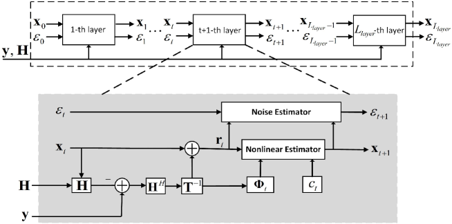
In this section, we propose a model-driven DL detector (referred to as VBINet) which is developed by unfolding the iterative IFVB detector. The network architecture is illustrated in Fig. 1, in which the network consists of $L_{\text{layer}}$ cascade layers with some trainable parameters. The trainable parameters of all layers are denoted as $\boldsymbol{\Omega}\triangleq\big{\{}\boldsymbol{T},\{c_{t}\}_{t=1}^{L_{\text{layer}}}\big{\}}$ , where $\boldsymbol{T}$ is a diagonal matrix common to all layers. We will explain these trainable parameters in detail later. For the $(t+1)$ th layer, the input includes $\boldsymbol{y}$ , $\boldsymbol{H}$ , $\boldsymbol{x}_{t}$ , and $\varepsilon_{t}$ , where $\boldsymbol{x}_{t}$ and $\varepsilon_{t}$ denote the $t$ th layer’s estimate of the signal and the noise variance, respectively. Given $\{\boldsymbol{y},\boldsymbol{H},\boldsymbol{x}_{t},\varepsilon_{t}\}$ , each layer performs the following updates:

		$\displaystyle\text{LE}:\quad\quad\boldsymbol{r}_{t}=\boldsymbol{x}_{t}+\boldsymbol{T}^{-1}\boldsymbol{H}^{H}\left(\boldsymbol{y}-\boldsymbol{H}\boldsymbol{x}_{t}\right),$		(52)
		$\displaystyle\text{NLE}:\quad\boldsymbol{x}_{t+1}=c_{t}E\{\boldsymbol{x};\boldsymbol{r}_{t},\boldsymbol{\Phi}_{t}\}+(1-c_{t})\boldsymbol{x}_{t},$		(53)
		$\displaystyle\text{Update of $\varepsilon_{t+1}$}:\quad\varepsilon_{t+1}=\frac{a+\frac{N_{r}}{2}}{b+\frac{1}{2}g_{\text{net}}(\boldsymbol{x}_{t+1},\boldsymbol{x}_{t})}$		(54)

where

	$\displaystyle\quad\quad\quad\quad\quad\quad\quad\quad\boldsymbol{\Phi}_{t}=\frac{1}{\varepsilon_{t}}\boldsymbol{T}^{-1},$		(55)
	$\displaystyle g_{\text{net}}(\boldsymbol{x}_{t+1},\boldsymbol{x}_{t})$
	$\displaystyle=\\|\boldsymbol{y}-\boldsymbol{H}\boldsymbol{x}_{t}\\|_{2}^{2}+2\Re\Big{\{}(\boldsymbol{x}_{t+1}-\boldsymbol{x}_{t})^{H}\boldsymbol{H}^{H}(\boldsymbol{H}\boldsymbol{x}_{t}-\boldsymbol{y})\Big{\}}$
	$\displaystyle\quad+\text{Tr}\Big{(}\boldsymbol{T}\big{(}\boldsymbol{x}_{t+1}-\boldsymbol{x}_{t}\big{)}\big{(}\boldsymbol{x}_{t+1}-\boldsymbol{x}_{t}\big{)}^{H}+\boldsymbol{T}\boldsymbol{\Sigma}_{\text{net}}^{t+1}\Big{)},$		(56)
	$\displaystyle\Sigma_{i,{\text{net}}}^{t+1}=c_{t}^{2}\Big{(}E\{x_{i}^{2};r_{i,t},\Phi_{i,t}\}-\big{[}E\{x_{i};r_{i,t},\Phi_{i,t}\}\big{]}^{2}\Big{)},\quad\forall i.$		(57)

in which $\Sigma_{i,{\text{net}}}^{t+1}$ is the $i$ th diagonal element of the diagonal matrix $\boldsymbol{\Sigma}_{\text{net}}^{t+1}$ .

We see that the update formulas (52)–(57) are similar to the IFVB detector’s update formulas (47)–(51). Nevertheless, there are two major differences. Firstly, in the LE step, the diagonal matrix $\boldsymbol{T}$ is no longer pre-specified; instead, it is a trainable diagonal matrix. The reason for doing this is to make the network learnable and flexible. Specifically, we believe that $\boldsymbol{T}$ given in (27) may not be the best, and hope that we can find a more suitable diagonal matrix through training. Secondly, in the NLE step, $\boldsymbol{x}_{t+1}$ is updated by applying an adaptive damping scheme with a learnable parameter $c_{t}$ . In the adaptive damping scheme, the damping parameter can help control the convergence rate and improve the robustness of the system [34].

One may wonder why not use an individual $\boldsymbol{T}$ for each layer of the network. The reason is that using a common diagonal matrix $\boldsymbol{T}$ for all layers can substantially reduce the number of learnable variables, which facilitates training when the number of training data is limited. Also, notice that the iterative algorithm developed in the previous section uses a same $\boldsymbol{T}$ throughout its iterative process. This suggests that using an individual $\boldsymbol{T}$ for each layer may not be necessary. To corroborate our conjecture, we conducted experiments to compare these two schemes. Simulation results show that using an individual $\boldsymbol{T}$ for each layer does not achieve a clear performance improvement over the scheme of using a common diagonal matrix $\boldsymbol{T}$ .

Moreover, due to the use of the term $(1-c_{t})\boldsymbol{x}_{t}$ in the NLE step, the covariance matrix of $\boldsymbol{x}_{t+1}$ , denoted by $\boldsymbol{\Sigma}_{x}$ , cannot be updated via (51). Note that in the IFVB detector, according to (48), the NLE outputs the mean value of the variable $\boldsymbol{x}$ . Meanwhile, in the VBINet, the output of the NLE is the mean of a new variable $\boldsymbol{x}_{\text{net}}$ defined as

\displaystyle\boldsymbol{x}_{\text{net}}=c_{t}\boldsymbol{x}+(1-c_{t})\boldsymbol{x}_{t}

(58)

Thus the mean of $\boldsymbol{x}_{\text{net}}$ is given by

\displaystyle\boldsymbol{x}_{t+1}=\langle\boldsymbol{x}_{\text{net}}\rangle=c_{t}E\{\boldsymbol{x};\boldsymbol{r}_{t},\boldsymbol{\Phi}_{t}\}+(1-c_{t})\boldsymbol{x}_{t}

(59)

and the $i$ th diagonal element of the diagonal covariance matrix $\boldsymbol{\Sigma}_{\text{net}}^{t+1}$ of the random variable $\boldsymbol{x}_{\text{net}}$ is given by

$\displaystyle\Sigma_{i,{\text{net}}}^{t+1}$	$\displaystyle=\text{var}(x_{i,\text{net}})$
	$\displaystyle=c_{t}^{2}(\langle x_{i}^{2}\rangle-\langle x_{i}\rangle^{2})$
	$\displaystyle=c_{t}^{2}\Big{(}E\{x_{i}^{2};r_{i,t},\Phi_{i,t}\}-\big{[}E\{x_{i};r_{i,t},\Phi_{i,t}\}\big{]}^{2}\Big{)},\quad\forall i$	(60)

in which $x_{i,\text{net}}$ denotes the $i$ th element of $\boldsymbol{x}_{\text{net}}$ . This explains how (57) is derived.

Remark 1: We see that the total number of learnable parameters of VBINet is $|\boldsymbol{\Omega}|=N_{t}+L_{\text{layer}}$ , as each layer shares the same learnable variable $\boldsymbol{T}$ while $c_{t}$ are generally different for different layers. Suppose that the number of users is $N_{t}=16$ and the number of layers is set to $L_{\text{layer}}=10$ . The total number of learnable parameters of VBINet is $26$ . As a comparison, the OAMPNet has $40$ parameters to be learned for the same problem being considered. Due to the small number of learnable parameters, the proposed VBINet can be effectively trained even with a limited number of training data samples.

Remark 2: An important advantage of the proposed VBINet over state-of-the-art deep unfolding-based detectors such as the OAMPNet and the MMNet is that the VBINet can automatically estimate the noise variance $1/\varepsilon$ , while both the OAMPNet and the MMNet require the knowledge of $1/\varepsilon$ , and an inaccurate knowledge of the noise variance results in a considerable amount of performance degradation, as will be demonstrated later in our experiments. Another advantage of the proposed VBINet is that the update formulas can be efficiently implemented via simple matrix/vector operations. No matrix inverse operation is needed.

Remark 3: The proposed VBINet can provide an approximate posterior probability of the transmitted symbols, which is useful for channel decoders relying on the estimate of the posterior probability of the transmitted symbols [35]. Thus the proposed VBINet can be well suited for joint symbol detection and channel decoding.

VI IFVB Detector: Extension To Correlated Channels

The proposed IFVB detector performs well on channel matrices with independent and identically distributed (i.i.d.) entries. Nevertheless, similar to AMP and other message-passing-based algorithms, its performance degrades considerably on realistic, spatially-correlated channel matrices. To address this issue, we discuss how to improve the proposed IFVB detector to accommodate arbitrarily correlated channel matrices.

The key idea behind the improved IFVB detector is to conduct a truncated singular value decomposition (SVD) of the channel matrix $\boldsymbol{H}=\boldsymbol{U}\boldsymbol{\Sigma}\boldsymbol{V}^{H}$ , where $\boldsymbol{U}\in\mathbb{C}^{N_{r}\times N_{t}}$ , $\boldsymbol{\Sigma}\in\mathbb{C}^{N_{t}\times N_{t}}$ , and $\boldsymbol{V}\in\mathbb{C}^{N_{t}\times N_{t}}$ . Define $\boldsymbol{A}\triangleq\boldsymbol{U}\boldsymbol{\Sigma}$ and $\boldsymbol{s}\triangleq\boldsymbol{V}^{H}\boldsymbol{x}$ . The received signal vector $\boldsymbol{y}\in\mathbb{C}^{N_{r}}$ in (1) can be equivalently written as

\displaystyle\boldsymbol{y}=\boldsymbol{A}\boldsymbol{s}+\boldsymbol{n}

(61)

Instead of detecting $\boldsymbol{x}$ , we aim to estimate $\boldsymbol{s}$ based on the above observation model. Let $\boldsymbol{\theta}\triangleq\{\boldsymbol{s},\varepsilon\}$ denote the hidden variables, and let $p(\boldsymbol{s})$ denote the prior distribution of $\boldsymbol{s}$ . Thus the ELBO is given as

	$\displaystyle L(q)$	$\displaystyle\triangleq\int q(\boldsymbol{\theta})\ln\frac{p(\boldsymbol{y},\boldsymbol{s},\varepsilon)}{q(\boldsymbol{\theta})}d\boldsymbol{\theta}$
		$\displaystyle=\int q(\boldsymbol{\theta})\ln\frac{p(\boldsymbol{y}\|\boldsymbol{s},\varepsilon)p(\boldsymbol{s})p(\varepsilon)}{q(\boldsymbol{\theta})}d\boldsymbol{\theta}$		(62)

where

\displaystyle p(\boldsymbol{y}|\boldsymbol{s},\varepsilon)

\displaystyle=\big{(}\frac{\varepsilon^{\frac{1}{2}}}{\sqrt{2\pi}}\big{)}^{N_{r}}\exp\big{\{}-\frac{\varepsilon\|\boldsymbol{y}-\boldsymbol{A}\boldsymbol{s}\|_{2}^{2}}{2}\big{\}}

(63)

in which $\varepsilon$ still follows a Gamma distribution as assumed in (22).

Similar to what we did in the previous section, we resort to a relaxed ELBO to facilitate the variational inference. Let $\boldsymbol{T}\succcurlyeq\boldsymbol{\Sigma}^{2}$ . Invoking Lemma 1, a lower bound on $p(\boldsymbol{y}|\boldsymbol{s},\varepsilon)$ can be obtained as

	$\displaystyle p(\boldsymbol{y}\|\boldsymbol{s},\varepsilon)$	$\displaystyle=\big{(}\frac{\varepsilon^{\frac{1}{2}}}{\sqrt{2\pi}}\big{)}^{N_{r}}\exp\Big{\{}-\frac{\varepsilon}{2}\\|\boldsymbol{y}-\boldsymbol{A}\boldsymbol{s}\\|_{2}^{2}\Big{\}}$
		$\displaystyle\geqslant\big{(}\frac{\varepsilon^{\frac{1}{2}}}{\sqrt{2\pi}}\big{)}^{N_{r}}\exp\Big{\{}-\frac{\varepsilon}{2}g(\boldsymbol{s},\boldsymbol{z})\Big{\}}\triangleq F(\boldsymbol{y},\boldsymbol{s},\varepsilon,\boldsymbol{z})$		(64)

where

	$\displaystyle g(\boldsymbol{s},\boldsymbol{z})$	$\displaystyle\triangleq\\|\boldsymbol{y}-\boldsymbol{A}\boldsymbol{z}\\|_{2}^{2}+2\Re\big{\{}(\boldsymbol{s}-\boldsymbol{z})^{H}\boldsymbol{A}^{H}(\boldsymbol{A}\boldsymbol{z}-\boldsymbol{y})\big{\}}+$
		$\displaystyle\quad\quad(\boldsymbol{s}-\boldsymbol{z})^{H}\boldsymbol{T}(\boldsymbol{s}-\boldsymbol{z})$		(65)

and the inequality becomes equality when $\boldsymbol{T}=\boldsymbol{\Sigma}^{2}$ . Here, we consider a specialized form of $\boldsymbol{T}\triangleq\boldsymbol{\overline{T}}+\frac{\delta}{\varepsilon}\boldsymbol{I}$ , where the first term is a diagonal matrix independent of $\varepsilon$ and the second term is a function of $\varepsilon$ . We will show that such an expression of $\boldsymbol{T}$ leads to an LMMSE-like estimator for the LE step.

Utilizing (64), a relaxed ELBO can be obtained as

\displaystyle L(q)\geqslant\tilde{L}(q,\boldsymbol{z})

\displaystyle=\int q(\boldsymbol{\theta})\ln\frac{G(\boldsymbol{y},\boldsymbol{s},\varepsilon,\boldsymbol{z})}{q(\boldsymbol{\theta})}d\boldsymbol{\theta}

(66)

where

\displaystyle G(\boldsymbol{y},\boldsymbol{s},\varepsilon,\boldsymbol{z})=F(\boldsymbol{y},\boldsymbol{s},\varepsilon,\boldsymbol{z})p(\boldsymbol{s})p(\varepsilon)

(67)

Similarly, we aim to maximize the relaxed ELBO with respect to $q(\boldsymbol{\theta})$ and the parameter $\boldsymbol{z}$ , which leads to a variational EM algorithm. In the E-step, given $\boldsymbol{z}$ , the approximate posterior distribution of $\boldsymbol{\theta}\triangleq\{\boldsymbol{s},\varepsilon\}$ is updated. In the M-step, the parameter $\boldsymbol{z}$ can be updated by maximizing $\tilde{L}(q,\boldsymbol{z})$ with $q(\boldsymbol{\theta})$ fixed. Details of the variational EM algorithm are provided below.

A. E-step

1) Update of $q_{\boldsymbol{s}}(\boldsymbol{s})$ : The variational distribution $q_{\boldsymbol{s}}(\boldsymbol{s})$ can be calculated as

$\displaystyle\ln q_{\boldsymbol{s}}(\boldsymbol{s})$	$\displaystyle\propto\big{\langle}\ln{G}(\boldsymbol{y},\boldsymbol{s},\varepsilon,\boldsymbol{z})\big{\rangle}_{q_{\varepsilon}(\varepsilon)}$
	$\displaystyle\propto\big{\langle}\ln F(\boldsymbol{y},\boldsymbol{s},\varepsilon,\boldsymbol{z})+\ln p(\boldsymbol{s})\big{\rangle}_{q_{\varepsilon}(\varepsilon)}$
	$\displaystyle\propto\big{\langle}-\frac{\varepsilon}{2}g(\boldsymbol{s},\boldsymbol{z})+\ln p(\boldsymbol{s})\big{\rangle}_{q_{\varepsilon}(\varepsilon)}$
	$\displaystyle\propto\Big{\langle}-\frac{\varepsilon}{2}\Big{(}2\Re\big{\{}(\boldsymbol{s}-\boldsymbol{z})^{H}\boldsymbol{A}^{H}(\boldsymbol{A}\boldsymbol{z}-\boldsymbol{y})\big{\}}+$
	$\displaystyle\quad\quad(\boldsymbol{s}-\boldsymbol{z})^{H}\boldsymbol{T}(\boldsymbol{s}-\boldsymbol{z})\Big{)}+\ln p(\boldsymbol{s})\Big{\rangle}_{q_{\varepsilon}(\varepsilon)}$
	$\displaystyle\overset{(a)}{\propto}\ln N(\boldsymbol{s};\boldsymbol{\bar{r}},\boldsymbol{\bar{\Phi}})+\ln p(\boldsymbol{s})$	(68)

where in $(a)$ , we have

$\displaystyle\boldsymbol{\bar{\Phi}}$	$\displaystyle=\frac{1}{\langle\varepsilon\rangle}\langle\boldsymbol{T}^{-1}\rangle$	(69)
$\displaystyle\boldsymbol{\bar{r}}$	$\displaystyle=\left\langle\boldsymbol{T}^{-1}\Big{(}\boldsymbol{A}^{H}\boldsymbol{y}+\boldsymbol{T}\boldsymbol{z}-\boldsymbol{A}^{H}\boldsymbol{A}\boldsymbol{z}\Big{)}\right\rangle$
	$\displaystyle=\boldsymbol{z}+\langle\boldsymbol{T}^{-1}\rangle\boldsymbol{A}^{H}\Big{(}\boldsymbol{y}-\boldsymbol{A}\boldsymbol{z}\Big{)}$	(70)

in which

\displaystyle\langle\boldsymbol{T}^{-1}\rangle=\boldsymbol{\overline{T}}^{-1}+\frac{\langle\varepsilon\rangle}{\delta}\boldsymbol{I}

(71)

Note that the approximate posterior distribution $q_{\boldsymbol{s}}(\boldsymbol{s})$ is difficult to obtain because the prior $p(\boldsymbol{s})$ has an intractable expression. To address this issue, we, instead, examine the posterior distribution $q_{\boldsymbol{x}}(\boldsymbol{x})$ . Recalling that $\boldsymbol{x}=\boldsymbol{V}\boldsymbol{s}$ , we have

\displaystyle\ln q_{\boldsymbol{x}}(\boldsymbol{x})

\displaystyle\propto\ln N(\boldsymbol{x};\boldsymbol{r},\boldsymbol{\Phi})+\ln p(\boldsymbol{x})

(72)

where

	$\displaystyle\boldsymbol{r}$	$\displaystyle=\boldsymbol{V}\boldsymbol{\bar{r}}$		(73)
	$\displaystyle\boldsymbol{\Phi}$	$\displaystyle=\boldsymbol{V}\boldsymbol{\bar{\Phi}}\boldsymbol{V}^{H},$		(74)

To calculate $q_{\boldsymbol{x}}(\boldsymbol{x})$ , we neglect the cross-correlation among entries of $\boldsymbol{x}$ , i.e., treat the off-diagonal entries of $\boldsymbol{\Phi}$ as zeros. This trick helps obtain an analytical approximate posterior distribution $q_{\boldsymbol{x}}(\boldsymbol{x})$ , and meanwhile has been empirically proven effective. Let $\Phi_{i}$ represent the $i$ th diagonal element of $\boldsymbol{\Phi}$ . The first and second moments of $x_{i}$ can be updated as

	$\displaystyle\langle x_{i}\rangle$	$\displaystyle=E\{x_{i};r_{i},\Phi_{i}\}=\frac{\sum_{i}x_{i}N(x_{i};r_{i},\Phi_{i})p(x_{i})}{\sum_{i}N(x_{i};r_{i},\Phi_{i})p(x_{i})},\quad\forall i$
	$\displaystyle\langle x_{i}^{2}\rangle$	$\displaystyle=E\{x_{i}^{2};r_{i},\Phi_{i}\}=\frac{\sum_{i}x_{i}^{2}N(x_{i};r_{i},\Phi_{i})p(x_{i})}{\sum_{i}N(x_{i};r_{i},\Phi_{i})p(x_{i})},\quad\forall i$		(75)

Thus we arrive at $q_{\boldsymbol{x}}(\boldsymbol{x})$ follows a Gaussian distribution with its mean $\langle\boldsymbol{x}\rangle=[\langle x_{1}\rangle\phantom{0}\ldots\phantom{0}\langle x_{N_{t}}\rangle]^{T}$ and covariance matrix $\boldsymbol{\Sigma}_{\boldsymbol{x}}=\text{diag}(\Sigma_{x_{1}},\ldots,\Sigma_{x_{N_{t}}})$ , where

\displaystyle\Sigma_{x_{i}}

\displaystyle=\langle x_{i}^{2}\rangle-\langle x_{i}\rangle^{2},\quad\forall i

(76)

Since $q_{\boldsymbol{x}}(\boldsymbol{x})$ follows a Gaussian distribution, the approximate posterior of $q_{\boldsymbol{s}}(\boldsymbol{s})$ also follows a Gaussian distribution, and its mean and covariance matrix can be readily obtained as

\displaystyle\langle\boldsymbol{s}\rangle=\boldsymbol{V}^{H}\langle\boldsymbol{x}\rangle

(77)

\displaystyle\boldsymbol{\Sigma}_{\boldsymbol{s}}=\boldsymbol{V}^{H}\boldsymbol{\Sigma}_{\boldsymbol{x}}\boldsymbol{V}

(78)

2) Update of $q_{\varepsilon}(\varepsilon)$ : The variational distribution $q_{\varepsilon}(\varepsilon)$ can be calculated as

$\displaystyle\ln q_{\varepsilon}(\varepsilon)$	$\displaystyle\propto\langle\ln{G}(\boldsymbol{y},\boldsymbol{s},\varepsilon,\boldsymbol{z})\rangle_{q_{\boldsymbol{s}}(\boldsymbol{s})}$
	$\displaystyle\propto\big{\langle}\ln F(\boldsymbol{y},\boldsymbol{s},\varepsilon,\boldsymbol{z})+\ln p(\varepsilon)\big{\rangle}_{q_{\boldsymbol{s}}(\boldsymbol{s})}$
	$\displaystyle\propto\Big{(}a-1+\frac{N_{r}}{2}\Big{)}\ln\varepsilon-\Big{(}\frac{1}{2}\langle\bar{g}(\boldsymbol{s},\boldsymbol{z})\rangle+b\Big{)}\varepsilon$	(79)

in which

	$\displaystyle\langle\bar{g}(\boldsymbol{s},\boldsymbol{z})\rangle=$	$\displaystyle\\|\boldsymbol{y}-\boldsymbol{A}\boldsymbol{z}\\|_{2}^{2}+2\Re\{(\langle\boldsymbol{s}\rangle-\boldsymbol{z})^{H}\boldsymbol{A}^{H}(\boldsymbol{A}\boldsymbol{z}-\boldsymbol{y})\}+$
		$\displaystyle\big{(}\langle\boldsymbol{s}\rangle-\boldsymbol{z}\big{)}^{H}\boldsymbol{\overline{T}}\big{(}\langle\boldsymbol{s}\rangle-\boldsymbol{z}\big{)}+\text{Tr}\Big{(}\boldsymbol{\overline{T}}\boldsymbol{\Sigma}_{\boldsymbol{s}}\Big{)}$		(80)

Thus the hyperparameter $\varepsilon$ follows a Gamma distribution, i.e.

\displaystyle q_{\varepsilon}(\varepsilon)=\text{Gamma}(\varepsilon;\tilde{a},\tilde{b})

(81)

where $\tilde{a}$ and $\tilde{b}$ are given by

\displaystyle\tilde{a}=a+\frac{N_{r}}{2},\quad\tilde{b}=b+\frac{1}{2}\langle\bar{g}(\boldsymbol{s},\boldsymbol{z})\rangle

(82)

Also, we have

\displaystyle\langle\varepsilon\rangle=\frac{\tilde{a}}{\tilde{b}}

(83)

B. M-step

Substituting $q(\boldsymbol{\theta};\boldsymbol{z}^{\text{old}})$ into $\tilde{L}(q,\boldsymbol{z})$ , the parameter $\boldsymbol{z}$ can be optimized via

\displaystyle\boldsymbol{z}^{\text{new}}

\displaystyle=\arg\max_{\boldsymbol{z}}\langle\ln{G}(\boldsymbol{y},\boldsymbol{s},\varepsilon,\boldsymbol{z})\rangle_{q(\boldsymbol{\theta};\boldsymbol{z}^{\text{old}})}

(84)

Setting the derivative of the logarithm function to zero yields

\displaystyle\frac{\partial\langle\ln{G}(\boldsymbol{y},\boldsymbol{\theta},\boldsymbol{z})\rangle_{q(\boldsymbol{\theta};\boldsymbol{z}^{\text{old}})}}{\partial\boldsymbol{z}}=\langle\varepsilon\rangle\big{(}\boldsymbol{\overline{T}}+\frac{\delta}{\langle\varepsilon\rangle}\boldsymbol{I}-\boldsymbol{\Sigma}^{2}\big{)}\big{(}\langle\boldsymbol{s}\rangle-\boldsymbol{z}\big{)}=\boldsymbol{0}

(85)

Since $\langle\varepsilon\rangle>0$ and $\boldsymbol{\overline{T}}+\frac{\delta}{\langle\varepsilon\rangle}\boldsymbol{I}\succeq\boldsymbol{\Sigma}^{2}$ , the solution of $\boldsymbol{z}$ is given by

\displaystyle\boldsymbol{z}^{\text{new}}=\langle\boldsymbol{s}\rangle

(86)

VI-A Summary of The Improved IFVB Detector

For the sake of clarity, the improved IFVB detector can be summarized as an iterative algorithm with each iteration consisting of a linear estimation step and a nonlinear estimation step:

$\displaystyle\quad\text{LE}:\quad\quad~{}\boldsymbol{\bar{r}}_{t}$	$\displaystyle=\boldsymbol{s}_{t}+\boldsymbol{T}_{t}^{-1}\boldsymbol{A}^{H}(\boldsymbol{y}-\boldsymbol{A}\boldsymbol{s}_{t})$	(87)
$\displaystyle\boldsymbol{r}_{t}$	$\displaystyle=\boldsymbol{V}\boldsymbol{\bar{r}}_{t}$	(88)
$\displaystyle\quad\text{NLE}:~{}~{}x_{i,t+1}$	$\displaystyle=E\{x_{i};r_{i,t},\Phi_{i,t}\},\quad\forall i$	(89)
$\displaystyle\boldsymbol{s}_{t+1}$	$\displaystyle=\boldsymbol{V}^{H}\boldsymbol{x}_{t+1}$	(90)

where $\boldsymbol{T}_{t}\triangleq\boldsymbol{\overline{T}}+\frac{\delta}{\varepsilon_{t}}\boldsymbol{I}$ , and $r_{i,t}$ and $\Phi_{i,t}$ denote the $i$ th elements of $\boldsymbol{r}_{t}$ and $\boldsymbol{\Phi}_{t}$ , respectively. The linear estimator in equations (87) and (88) derives from (70) and (73). The nonlinear estimator in equations (89) and (90) follows from (75) and (77). In (89), the variance $\Phi_{i,t}$ can be obtained as

\displaystyle\Phi_{i,t}=\boldsymbol{v}_{i}^{r}\boldsymbol{\bar{\Phi}}_{t}(\boldsymbol{v}_{i}^{r})^{H},\quad\forall i

(91)

where $\boldsymbol{v}_{i}^{r}$ denotes the $i$ th row of $\boldsymbol{V}$ , and $\boldsymbol{\bar{\Phi}}_{t}=\frac{1}{\varepsilon_{t}}\boldsymbol{T}_{t}^{-1}$ . Here $\varepsilon_{t+1}$ is updated as

\displaystyle\varepsilon_{t+1}=\frac{\tilde{a}}{\tilde{b}_{t+1}}=\frac{a+\frac{N_{r}}{2}}{b+\frac{1}{2}\bar{g}(\boldsymbol{s}_{t+1},\boldsymbol{s}_{t})}

(92)

where

	$\displaystyle\bar{g}(\boldsymbol{s}_{t+1},\boldsymbol{s}_{t})=$	$\displaystyle\\|\boldsymbol{y}-\boldsymbol{A}\boldsymbol{s}_{t}\\|_{2}^{2}+2\Re\big{\{}(\boldsymbol{s}_{t+1}-\boldsymbol{s}_{t})^{H}\boldsymbol{A}^{H}(\boldsymbol{A}\boldsymbol{s}_{t}-\boldsymbol{y})\big{\}}$
		$\displaystyle+\big{(}\boldsymbol{s}_{t+1}-\boldsymbol{s}_{t}\big{)}^{H}\boldsymbol{\overline{T}}\big{(}\boldsymbol{s}_{t+1}-\boldsymbol{s}_{t}\big{)}+\text{Tr}\big{(}\boldsymbol{\overline{T}}\boldsymbol{\Sigma}_{\boldsymbol{s}}^{t+1}\big{)}$		(93)

in which

\displaystyle\boldsymbol{\Sigma}_{\boldsymbol{s}}^{t+1}=\boldsymbol{V}^{H}\boldsymbol{\Sigma}_{\boldsymbol{x}}^{t+1}\boldsymbol{V}

(94)

and the $i$ th diagonal element of the diagonal matrix $\boldsymbol{\Sigma}_{x}^{t+1}$ can be calculated as

\displaystyle\Sigma_{x_{i}}^{t+1}=E\{x_{i}^{2};r_{i,t},\Phi_{i,t}\}-\big{[}E\{x_{i};r_{i,t},\Phi_{i,t}\}\big{]}^{2},\quad\forall i

(95)

Discussions: For the Improved IFVB Detector, a specialized form of $\boldsymbol{T}\triangleq\boldsymbol{\overline{T}}+\frac{\delta}{\varepsilon}\boldsymbol{I}$ is considered. The reason is that such a specialized form will lead to an LMMSE-like estimator for the LE step, i.e. $\boldsymbol{\bar{r}}_{t}=\boldsymbol{s}_{t}+\boldsymbol{T}_{t}^{-1}\boldsymbol{A}^{H}(\boldsymbol{y}-\boldsymbol{A}\boldsymbol{s}_{t})$ (see (87)). Here, $\boldsymbol{\bar{r}}_{t}$ denotes the current estimate of $\boldsymbol{s}$ in the LE step, and $\boldsymbol{s}_{t}$ denotes the previous estimate of $\boldsymbol{s}$ . If we treat $\boldsymbol{s}-\boldsymbol{s}_{t}$ as a random variable following a Gaussian distribution with zero mean and covariance matrix $\delta^{-1}\boldsymbol{I}$ , and let $\boldsymbol{\overline{T}}=\boldsymbol{\Sigma}^{2}=\boldsymbol{A}^{H}\boldsymbol{A}$ . It can be readily verified that $\boldsymbol{\bar{r}}_{t}-\boldsymbol{s}_{t}=\boldsymbol{T}_{t}^{-1}\boldsymbol{A}^{H}(\boldsymbol{y}-\boldsymbol{A}\boldsymbol{s}_{t})$ is in fact an LMMSE estimator of $\boldsymbol{s}-\boldsymbol{s}_{t}$ given the observation: $\boldsymbol{y}-\boldsymbol{A}\boldsymbol{s}_{t}=\boldsymbol{A}(\boldsymbol{s}-\boldsymbol{s}_{t})+\boldsymbol{n}$ . It is known that the LMMSE estimator can compensate for the noise and effectively improve the estimation performance. This is the reason why we choose such a specialized form of $\boldsymbol{T}$ .

VII VBINet Detector for Correlated Channels

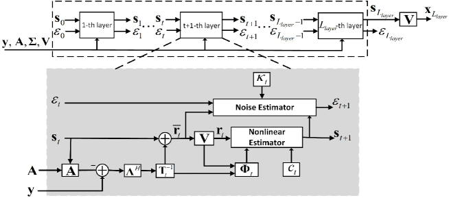
In this section, we propose a model-driven DL detector (referred to as Improved-VBINet) by unfolding the improved IFVB detector. The network architecture of Improved-VBINet is illustrated in Fig. 2, in which the network consists of $L_{\text{layer}}$ cascade layers. The trainable parameters of all layers are denoted as $\boldsymbol{\Omega}\triangleq\big{\{}\boldsymbol{\Psi},\{\delta_{t}\}_{t=1}^{L_{\text{layer}}},\{c_{t}\}_{t=1}^{L_{\text{layer}}},\{\kappa_{t}\}_{t=1}^{L_{\text{layer}}}\big{\}}$ , where the diagonal matrix $\boldsymbol{\Psi}$ and $\delta_{t}$ are related to the diagonal matrix $\boldsymbol{T}_{t}$ . For the $(t+1)$ th layer, the input includes $\boldsymbol{y}$ , $\boldsymbol{A}$ , $\boldsymbol{\Sigma}$ , $\boldsymbol{V}$ , $\boldsymbol{s}_{t}$ , and $\varepsilon_{t}$ , where $\boldsymbol{s}_{t}$ and $\varepsilon_{t}$ denote the $t$ th layer’s estimate of the signal and the noise variance, respectively. Given $\{\boldsymbol{y},\boldsymbol{A},\boldsymbol{\Sigma},\boldsymbol{V},\boldsymbol{s}_{t},\varepsilon_{t}\}$ , each layer performs the following updates:

		$\displaystyle\text{LE}:\quad\quad\quad~{}\boldsymbol{\bar{r}}_{t}=\boldsymbol{s}_{t}+\boldsymbol{T}_{t}^{-1}\boldsymbol{A}^{H}(\boldsymbol{y}-\boldsymbol{A}\boldsymbol{s}_{t}),$		(96)
		$\displaystyle\quad\quad\quad\quad\quad~{}\boldsymbol{r}_{t}=\boldsymbol{V}\boldsymbol{\bar{r}}_{t}$		(97)
		$\displaystyle\text{NLE}:\quad x_{i,t+1}=E\{x_{i};r_{i,t},\Phi_{i,t}\},\quad\forall i$		(98)
		$\displaystyle\quad\quad\quad~{}~{}~{}~{}\boldsymbol{s}_{t+1}=c_{t}\boldsymbol{V}^{H}\boldsymbol{x}_{t+1}+(1-c_{t})\boldsymbol{s}_{t}$		(99)
		$\displaystyle\text{Update of $\varepsilon_{t+1}$}:\quad\varepsilon_{t+1}=\frac{a+\frac{N_{r}}{2}}{b+\frac{1}{2}g_{\text{net}}(\boldsymbol{s}_{t+1},\boldsymbol{s}_{t})}$		(100)

where

	$\displaystyle\quad\quad\quad\quad\boldsymbol{T}_{t}\triangleq\boldsymbol{\overline{T}}+\frac{\delta_{t}}{\varepsilon_{t}}\boldsymbol{I},\quad\boldsymbol{\overline{T}}\triangleq\boldsymbol{\Sigma}^{2}+\boldsymbol{\Psi}^{2}$		(101)
	$\displaystyle\quad\quad\quad\quad\boldsymbol{\bar{\Phi}}_{t}=\frac{1}{\varepsilon_{t}}\boldsymbol{T}_{t}^{-1},\quad\quad\quad\quad\quad\quad$		(102)
	$\displaystyle\quad\quad\quad\quad\Phi_{i,t}=\boldsymbol{v}_{i}^{r}\boldsymbol{\bar{\Phi}}_{t}(\boldsymbol{v}_{i}^{r})^{H},\quad\forall i\quad\quad\quad\quad\quad\quad$		(103)
	$\displaystyle g_{\text{net}}(\boldsymbol{s}_{t+1},\boldsymbol{s}_{t})$
	$\displaystyle=\\|\boldsymbol{y}-\boldsymbol{A}\boldsymbol{s}_{t}\\|_{2}^{2}+2\Re\big{\{}(\boldsymbol{s}_{t+1}-\boldsymbol{s}_{t})^{H}\boldsymbol{A}^{H}(\boldsymbol{A}\boldsymbol{s}_{t}-\boldsymbol{y})\big{\}}$
	$\displaystyle+\big{(}\boldsymbol{s}_{t+1}-\boldsymbol{s}_{t}\big{)}^{H}\boldsymbol{\overline{T}}\big{(}\boldsymbol{s}_{t+1}-\boldsymbol{s}_{t}\big{)}+\text{Tr}\Big{(}\boldsymbol{\overline{T}}\boldsymbol{\Sigma}_{\text{net}}^{t+1}\Big{)},\quad\quad\quad$		(104)
	$\displaystyle\quad\quad\quad\quad\boldsymbol{\Sigma}_{\text{net}}^{t+1}=c_{t}^{2}\kappa_{t}^{2}\boldsymbol{I}.$		(105)

We see that the update formulas (96)–(105) are similar to the improved IFBL detector’s update formulas (87)–(95). Nevertheless, there are several major differences. Firstly, in the LE step, $\boldsymbol{T}_{t}$ which is calculated according to certain rules is replaced by a trainable diagonal matrix $\boldsymbol{T}_{t}$ due to the use of the learnable variables $\big{\{}\boldsymbol{\Psi},\{\delta_{t}\}_{t=1}^{L_{\text{layer}}}\big{\}}$ . Specifically, the linear estimator module turns out to have a form similar to the LMMSE estimator, i.e.

	$\displaystyle\boldsymbol{\bar{r}}_{t}$	$\displaystyle=\boldsymbol{s}_{t}+\boldsymbol{T}_{t}^{-1}\boldsymbol{A}^{H}\Big{(}\boldsymbol{y}-\boldsymbol{A}\boldsymbol{s}_{t}\Big{)}$
		$\displaystyle=\boldsymbol{s}_{t}+\Big{(}\boldsymbol{\overline{T}}+\frac{\delta_{t}}{\varepsilon_{t}}\boldsymbol{I}\Big{)}^{-1}\boldsymbol{A}^{H}\Big{(}\boldsymbol{y}-\boldsymbol{A}\boldsymbol{s}_{t}\Big{)}$		(106)

Secondly, in the NLE step, $\boldsymbol{s}_{t+1}$ is updated by applying an adaptive damping scheme with a learnable parameter $c_{t}$ . Due to the use of the term $(1-c_{t})\boldsymbol{s}_{t}$ in the NLE step, the output of the NLE is the mean of a new variable $\boldsymbol{s}_{\text{net}}$ defined as

\displaystyle\boldsymbol{s}_{\text{net}}=c_{t}\boldsymbol{s}+(1-c_{t})\boldsymbol{s}_{t}

(107)

Recalling that $\boldsymbol{s}=\boldsymbol{V}^{H}\boldsymbol{x}$ , thus the mean of $\boldsymbol{s}_{\text{net}}$ is given by

\displaystyle\boldsymbol{s}_{t+1}=\langle\boldsymbol{s}_{\text{net}}\rangle=c_{t}\boldsymbol{V}^{H}E\{\boldsymbol{x};\boldsymbol{r}_{t},\boldsymbol{\Phi}_{t}\}+(1-c_{t})\boldsymbol{s}_{t}

(108)

and the covariance matrix $\boldsymbol{\Sigma}_{\text{net}}^{t+1}$ of the random variable $\boldsymbol{s}_{\text{net}}$ is given by

\displaystyle\boldsymbol{\Sigma}_{\text{net}}^{t+1}=c_{t}^{2}\boldsymbol{\Sigma}_{s}^{t+1}=c_{t}^{2}\boldsymbol{V}^{H}\boldsymbol{\Sigma}_{\boldsymbol{x}}^{t+1}\boldsymbol{V}

(109)

Here $\boldsymbol{\Sigma}_{\boldsymbol{x}}^{t+1}$ is a diagonal matrix whose diagonal elements can be calculated according to (95). To further reduce the complexity, we approximate $\boldsymbol{\Sigma}_{\boldsymbol{x}}^{t+1}$ as $\kappa_{t}^{2}\boldsymbol{I}$ , where $\kappa_{t}$ is a learnable parameter. Thus we have

\displaystyle\boldsymbol{\Sigma}_{\text{net}}^{t+1}=c_{t}^{2}\kappa_{t}^{2}\boldsymbol{I}

(110)

This explains how (105) is derived.

Remark 1: We see that the total number of learnable parameters of the improved-VBINet is $|\boldsymbol{\Omega}|=N_{t}+3L_{\text{layer}}$ , as each layer shares the same learnable variable $\boldsymbol{\Psi}$ but $\{\delta_{t},c_{t},\kappa_{t}\}$ are generally different for different layers. The total number of learnable parameters of the Improved-VBINet is comparable to that of OAMPNet.

VII-A Computational Complexity Analysis

We discuss the computational complexity of our proposed VBINet detectors. Specifically, for the i.i.d. Gaussian channels, at each layer the complexity of the proposed VBINet detector is dominated by the multiplication of an $N_{t}\times N_{r}$ matrix and an $N_{r}\times 1$ vector. Therefore the overall complexity of the proposed VBINet is of order $\mathcal{O}(N_{r}N_{t}L_{\text{layer}})$ . For the correlated channels, the proposed Improved-VBINet detector requires to conduct a truncated SVD decomposition of an $N_{r}\times N_{t}$ matrix in the initialization stage. Therefore the overall complexity of the proposed Improved-VBINet detector is of order $\mathcal{O}(N_{r}N_{t}L_{\text{layer}}+N_{t}^{3})$ . Similar to the proposed VBINet, the complexity of MMNet is of order $\mathcal{O}(N_{r}N_{t}L_{\text{layer}})$ . As for the OAMPNet, it requires to perform an inverse of an $N_{r}\times N_{r}$ matrix per layer, which results in a complexity of $\mathcal{O}(N_{r}^{3}L_{\text{layer}})$ in total. Since we usually have $N_{r}\gg N_{t}$ for massive MIMO detection, the complexity of the OAMPNet is much higher than our proposed method. This is also the reason why, for large-scale scenarios, training and test of OAMPNet becomes computationally prohibitive.

VIII Simulation Results

In this section, we compare the proposed VBINet-based detector¹¹1Codes are available at https://www.junfang-uestc.net/codes/VBINet.rar with state-of-the-art methods for i.i.d. Gaussian, correlated Rayleigh and realistic 3GPP MIMO channel matrices. In the following, we first discuss the implementation details of the proposed method and other competing algorithms.

VIII-A Implementation Details

During training, the learnable parameters are optimized using stochastic gradient descent. Thanks to the auto-differentiable machine-learning frameworks such as TensorFlow [36] and PyTorch [37], the learnable parameters can be easily trained when the loss function is determined. In our experiments, the loss function used for training is given by

\displaystyle f_{loss}=\frac{1}{L_{\text{layer}}}\sum_{t=1}^{L_{\text{layer}}}\|\boldsymbol{x}_{t}-\boldsymbol{x}\|_{2}^{2}

(111)

in which $\|\boldsymbol{x}_{t}-\boldsymbol{x}\|_{2}^{2}$ denotes the square error between the output of the $t$ -th layer and the true signal $\boldsymbol{x}$ .

In addition to the classical detectors such as the ZF and LMMSE, we compare our proposed method with the iterative algorithm OAMP and the following two state-of-the-art DL-based detectors: OAMPNet [22] and MMNet [23]. The ML detector is also included to provide a performance upper bound for all detectors. Given a set of training samples, the neural network is trained by the Adam optimizer [38] in the PyTorch framework.

In our simulations, the training and test samples $\{\boldsymbol{y},\boldsymbol{x}\}$ are generated according to the model (1), in which both the transmitted signal $\boldsymbol{x}$ , the channel $\boldsymbol{H}$ , and the observation noise $\boldsymbol{n}$ are randomly generated. Specifically, the channel $\boldsymbol{H}$ is either generated from an i.i.d. Gaussian distribution or generated according to a correlated channel model as described below. The number of training iterations is denoted as $N_{\text{iter}}$ , and the batch size for each iteration is denoted as $N_{\text{batch}}$ . The signal-to-noise ratio (SNR) is defined as

\displaystyle\text{SNR}(\text{dB})=10\log\Big{(}\frac{E[\|\boldsymbol{H}\boldsymbol{x}\|_{2}^{2}]}{E[\|\boldsymbol{n}\|_{2}^{2}]}\Big{)}

(112)

The training samples in each training iteration includes samples drawn from different SNRs within a certain range. For all detectors, the output signal will be rounded to the closest point on the discrete constellation set $\mathcal{C}$ . Details of different detectors are elaborated below.

$\bullet~{}\textbf{\text{ZF}}$ : It is a simple yet classical decoder which has a form as $\boldsymbol{\hat{x}}=(\boldsymbol{H}^{H}\boldsymbol{H})^{-1}\boldsymbol{H}^{H}\boldsymbol{y}$ .

$\bullet~{}\textbf{\text{LMMSE}}$ : The LMMSE detector takes a form of $\boldsymbol{\hat{x}}=\boldsymbol{H}^{H}\big{(}\boldsymbol{H}\boldsymbol{H}^{H}+\frac{1}{\varepsilon\cdot P_{x}}\boldsymbol{I}\big{)}^{-1}\boldsymbol{y}$ . Here $P_{x}$ is the average power of the QAM signal. In our simulation, we set $P_{x}=1$ .

$\bullet~{}\textbf{\text{IFVB}}$ : The algorithm is summarized in IV-C. The maximum number of iterations is set to $L_{\text{layer}}=100$ .

$\bullet~{}\textbf{\text{OAMP}}$ : It is an iterative algorithm developed based on the AMP algorithm. The maximum number of iterations is set to $L_{\text{layer}}=100$ .

$\bullet~{}\textbf{\text{OAMPNet}}$ : OAMPNet is a DL-based detector developed by unfolding the OAMP detector [22]. In our simulations, the number of layers of the OMAPNet is set to $10$ , and each layer has $4$ learnable variables.

$\bullet~{}\textbf{\text{MMNet-iid}}$ : The MMNet-iid [23] is specifically designed for i.i.d. Gaussian channels. In our simulations, the number of layers of the MMNet-iid is set to $10$ , and each layer has $2$ learnable variables.

$\bullet~{}\textbf{\text{MMNet}}$ : The MMNet [23] can be applied to arbitrarily correlated channel matrices, which needs to learn a matrix $\boldsymbol{A}_{t}$ for each layer, and the total number of learnable parameters is $2N_{t}(N_{r}+1)$ per layer.

$\bullet~{}\textbf{\text{VBINet}}$ : The architecture of our proposed VBINet is shown in Section V, which has $L_{\text{layer}}$ layers and $N_{t}+L_{\text{layer}}$ learnable variables.

$\bullet~{}\textbf{\text{Improved-VBINet}}$ : Applicable for arbitrarily correlated matrices, the proposed Improved-VBINet has $L_{\text{layer}}$ layers and $N_{t}+3L_{\text{layer}}$ learnable variables.

$\bullet~{}\textbf{\text{ML}}$ : It is implemented by using a highly optimized Mixed Integer Programming package Gurobi [39] ²²2The code is shared by [23]..

VIII-B Results

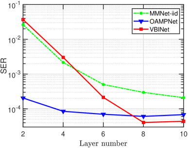
VIII-B1 Convergence Evaluation

The convergence property of our proposed network is evaluated. Fig. 3 depicts the symbol error rate (SER) of different detectors as a function of the number of layers $L_{\text{layer}}$ with QPSK modulation and i.i.d. Gaussian channels, where we set $N_{t}=16$ , $N_{r}=32$ , $N_{\text{batch}}=500$ , and $N_{\text{iter}}=10^{4}$ . We see that our proposed VBINet-based detector converges in less than $10$ layers, and after convergence, the proposed detector can achieve a certain amount of performance improvement over the OAMPNet and MMNet-iid.

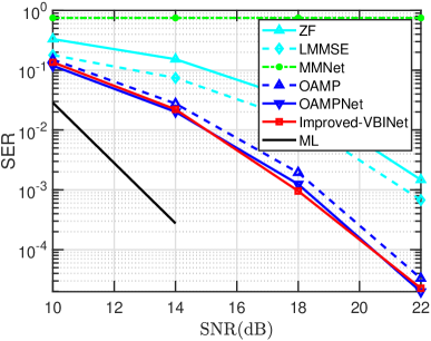
VIII-B2 I.I.D. Gaussian Channels

We first examine the detection performance of our proposed detector on i.i.d. Gaussian channels. We consider an offline training mode, in which training is performed over randomly generated channels and the performance is evaluated over another set of randomly generated channels.

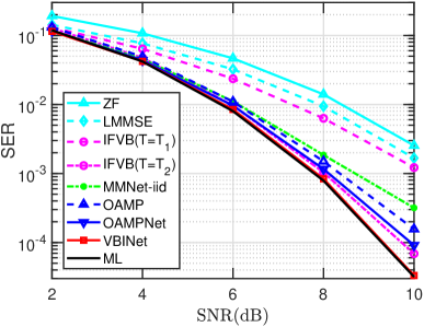
Fig. 4 plots the SER of respective algorithms as a function of the SNR, where QPSK modulation is considered, and we set $N_{t}=16$ , $N_{r}=32$ , $N_{\text{batch}}=500$ , and $N_{\text{iter}}=10^{4}$ . It can be observed that the ML detector achieves the best performance among all detectors, and the SER gap between our proposed VBINet and the ML detector is negligible. Moreover, the proposed VBINet outperforms the OAMPNet. We also see that the VBINet presents a clear performance advantage over the IFVB, which is because a more suitable $\boldsymbol{T}$ learned by VBINet will lead to better performance. For the IFVB, we use two different choices of $\boldsymbol{T}$ to show the impact of $\boldsymbol{T}$ on the detection performance. Specifically, the first choice of $\boldsymbol{T}$ is set to $\boldsymbol{T}_{1}=(\lambda_{\text{max}}(\boldsymbol{H}^{H}\boldsymbol{H})+\epsilon)\boldsymbol{I}$ and the second choice of $\boldsymbol{T}$ is set to $\boldsymbol{T}_{2}=\boldsymbol{H}_{d}$ , where $\boldsymbol{H}_{d}$ is a diagonal matrix which takes the diagonal entries of $\boldsymbol{H}^{H}\boldsymbol{H}$ . We see that the latter choice leads to much better performance, which indicates that the performance of IFVB depends largely on the choice of $\boldsymbol{T}$ . This is also the motivation why we learn $\boldsymbol{T}$ in the VBINet.

VIII-B3 Correlated Rayleigh Channels

We now examine the performance of respective detectors on correlated Rayleigh channels. The correlated Rayleigh channel is modeled as

\displaystyle\boldsymbol{H}=\boldsymbol{R}_{H}^{\frac{1}{2}}\boldsymbol{G}_{H}\boldsymbol{T}_{H}^{\frac{1}{2}}

(113)

where entries of $\boldsymbol{G}_{H}$ follow i.i.d. Gaussian distribution with zero mean and unit variance, $\boldsymbol{R}_{H}$ and $\boldsymbol{T}_{H}$ respectively denote the receive and transmit correlation matrices. Note that the receive and transmit correlation matrices can be characterized by a correlation coefficient $\rho$ [40], and a larger $\rho$ means that the channel matrix has a larger condition number. Again, in this experiment, offline training is considered.

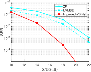
In Fig. 5, we plot the SER of respective algorithms as a function of SNR, where we set $\rho=0.8$ , $N_{t}=16$ , $N_{r}=32$ , $N_{\text{batch}}=500$ , and $N_{\text{iter}}=10^{4}$ . It can be observed that all DL detectors suffer a certain amount of performance degradation as the channel becomes ill-conditioned. Besides, MMNet fails to work in the offline training mode, where the test channels are different from the channels generated during the training phase. This is because in the LE step, the MMNet treats $\boldsymbol{A}_{t}$ as an entire trainable matrix. As a result, the trained neural network can only accommodate a particular channel realization. We also observe that both our proposed Improved-VBINet and OAMPNet work well in the offline training mode, and the proposed Improved-VBINet achieves performance slightly better than the OAMPNet.

VIII-B4 3GPP MIMO Channels

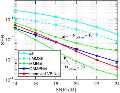
Next, we compare the performance of different detectors on realistic 3GPP 3D MIMO channels which are generated by the QuaDRiGa channel simulator [41, 42]. The parameters used to generate the channels are set the same as those in [23], except that the bandwidth is set to $1$ MHz, the number of effective sub-carriers is set to $F=128$ , and the number of sequences is $2$ . In this experiments, online training is considered, where the model parameters are trained and tested on the same realization of the channel. Specifically, we first train the neural network associated with the first subcarrier’s channel. The trained model parameters are then used as initial values of the neural network of the second subcarrier, and the second subcarrier’s network is employed as a start to train the third subcarrier’s network, and so on. Due to the channel correlation among adjacent subcarriers, the rest subcarriers’ neural networks can be efficiently trained with a small amount of data samples.

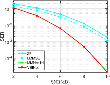
Fig. 6 depicts the SER of respective algorithms as a function of SNR, where we set $N_{t}=16$ , $N_{r}=32$ , and the QPSK modulation is considered. For the first subcarrier, the number of training iterations is $1000$ and the batch size is $500$ , while for all subsequent subcarriers, the number of online training iterations is $10$ and the batch size is $500$ . In Fig. 6, we also report results of the MMNet when the number of online training iterations is set to $N_{\text{online}}=20$ . We see that our proposed Improved-VBINet achieves performance similar to the OAMPNet. Also, it can be observed that MMNet achieves the best performance when a sufficient amount of data is allowed to be used for training. Nevertheless, the performance of MMNet degrades dramatically with a reduced amount of training data. Note that MMNet needs to learn an entire matrix $\boldsymbol{A}_{t}$ at each layer. With a large number of learnable parameters, the MMNet can well approximate the best detector when sufficient training is performed, whereas incurs a significant amount of performance degradation when training is insufficient.

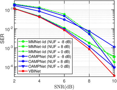
VIII-B5 Noise Uncertainty

Next, we examine the impact of noise variance uncertainty on the performance of different DL-based detectors. As mentioned earlier, different from our proposed VBINet which is capable of estimating the noise variance automatically, both OAMPNet and MMNet require the knowledge of noise variance for training and test. Note that the noise variance can be assumed known during the training phase, as we usually have access to the model parameters used to generate the training data samples. But the same assumption does not hold true for the test data. As a result, when evaluating the performance on the test data, both OAMPNet and MMNet have to replace the noise variance by its estimate. Let the estimated noise variance be $1/\hat{\varepsilon}=\eta(1/\varepsilon)$ . We also define the noise uncertainty factor (NUF) as $\text{NUF}\triangleq 10\log_{10}\eta$ . In this experiment, an offline training mode is considered.

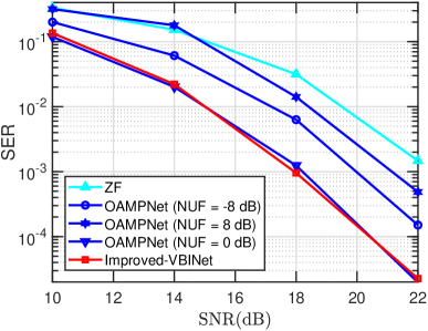
In Fig. 7, we plot the SER of respective algorithms as a function of SNR with different NUFs, where i.i.d. Gaussian channels and QPSK modulation are considered, and we set $N_{t}=16$ , $N_{r}=32$ , $N_{\text{batch}}=500$ , and $N_{\text{iter}}=10^{4}$ . It can be observed that both MMNet-iid and OAMPNet incur a considerable amount of performance loss when the estimated noise variance deviates from the true one. The performance gap between OAMPNet and VBINet becomes more pronounced when the estimate of the noise variance is inaccurate. Fig. 8 plots the SER of respective DL detectors as a function of SNR for correlated Rayleigh channels, where we set $\rho=0.8$ . Since MMNet fails to work in the offline training mode for correlated channels, its results are not included. Again, we see that OAMPNet suffer a substantial performance degradation when an inaccurate noise variance is used.

VIII-B6 Large-Scale MIMO Scenarios

We examine the detection performance of our proposed method in the large-scale MIMO scenario, in which the number of antennas at the BS is up to 128. In our experiments, the QPSK modulation is adopted, and we set $N_{t}=64$ , $N_{r}=128$ , $N_{\text{batch}}=500$ , and $N_{\text{iter}}=10^{4}$ . For the correlated Rayleigh channel, $\rho$ is set to $\rho=0.8$ . Fig. 9 and Fig. 10 plot the SERs of respective algorithms as a function of SNR for i.i.d. Gaussian and correlated Rayleigh channels, respectively. Note that in the LE step of the OAMPNet, $\boldsymbol{\hat{W}}_{t}$ is updated as $\hat{\boldsymbol{W}}_{t}=v_{t}^{2}\boldsymbol{H}^{H}(v_{t}^{2}\boldsymbol{H}\boldsymbol{H}^{H}+\boldsymbol{R}_{n})^{-1}$ , which involves computing the inverse of a matrix of size $N_{r}\times N_{r}$ at each layer. Hence for large-scale scenarios, training and test of OAMPNet becomes computationally prohibitive. For this reason, the results of OAMPNet are not included. Also, the results of MMNet are not included for correlated Rayleigh channels as it aims to learn an entire matrix $\boldsymbol{A}_{t}$ for each layer and thus fails to work well in the offline training mode. Results in Fig. 9 and Fig. 10 show that the proposed VBINet can achieve superior performance while with a low computational complexity.

IX Conclusions

In this paper, we proposed a model-driven DL network for MIMO detection based on a variational Bayesian framework. Two networks are respectively developed for i.i.d. Gaussian channels and arbitrarily correlated channels. The proposed networks, referred to as VBINet, have only a few learnable parameters and thus can be efficiently trained with a moderate amount of training. Simulation results show that the proposed detectors provide competitive performance for both i.i.d. Gaussian channels and realistic 3GPP MIMO channels. Moreover, the VBINet-based detectors can automatically determine the noise variance, and achieve a substantial performance improvement over existing DL-based detectors such as OAMPNet and MMNet in the presence of noise uncertainty.

References

[1] Q. Zhang, X. Cui, and X. Li, “Very tight capacity bounds for MIMO-correlated Rayleigh-fading channels,” IEEE Transactions on Wireless Communications, vol. 4, no. 2, pp. 681–688, 2005.
[2] A. Shahmansoori, G. E. Garcia, G. Destino, G. Seco-Granados, and H. Wymeersch, “Position and orientation estimation through millimeter-wave MIMO in 5G systems,” IEEE Transactions on Wireless Communications, vol. 17, no. 3, pp. 1822–1835, 2017.
[3] L. Lu, G. Y. Li, A. L. Swindlehurst, A. Ashikhmin, and R. Zhang, “An overview of massive MIMO: Benefits and challenges,” IEEE journal of selected topics in signal processing, vol. 8, no. 5, pp. 742–758, 2014.
[4] H. Q. Ngo, E. G. Larsson, and T. L. Marzetta, “Energy and spectral efficiency of very large multiuser MIMO systems,” IEEE Transactions on Communications, vol. 61, no. 4, pp. 1436–1449, 2013.
[5] D. Kong, X.-G. Xia, and T. Jiang, “A differential QAM detection in uplink massive MIMO systems,” IEEE Transactions on Wireless Communications, vol. 15, no. 9, pp. 6371–6383, 2016.
[6] M. E. Tipping, “Sparse Bayesian learning and the relevance vector machine,” Journal of machine learning research, vol. 1, no. Jun, pp. 211–244, 2001.
[7] D. L. Donoho, A. Maleki, and A. Montanari, “Message passing algorithms for compressed sensing: I. motivation and construction,” in 2010 IEEE information theory workshop on information theory (ITW 2010, Cairo). IEEE, 2010, pp. 1–5.
[8] W. Chen, D. Wipf, Y. Wang, Y. Liu, and I. J. Wassell, “Simultaneous Bayesian sparse approximation with structured sparse models,” IEEE Trans. Signal Processing, vol. 64, no. 23, pp. 6145–6159, 2016.
[9] S. Wu, L. Kuang, Z. Ni, J. Lu, D. Huang, and Q. Guo, “Low-complexity iterative detection for large-scale multiuser MIMO-OFDM systems using approximate message passing,” IEEE Journal of Selected Topics in Signal Processing, vol. 8, no. 5, pp. 902–915, 2014.
[10] T. P. Minka, “A family of algorithms for approximate Bayesian inference,” Ph.D. dissertation, Massachusetts Institute of Technology, 2001.
[11] J. Jaldén and B. Ottersten, “The diversity order of the semidefinite relaxation detector,” IEEE Transactions on Information Theory, vol. 54, no. 4, pp. 1406–1422, 2008.
[12] T. Wang, C.-K. Wen, H. Wang, F. Gao, T. Jiang, and S. Jin, “Deep learning for wireless physical layer: Opportunities and challenges,” China Communications, vol. 14, no. 11, pp. 92–111, 2017.
[13] Y. Wei, M.-M. Zhao, M. Hong, M.-J. Zhao, and M. Lei, “Learned conjugate gradient descent network for massive MIMO detection,” IEEE Transactions on Signal Processing, vol. 68, pp. 6336–6349, 2020.
[14] H. Ye, G. Y. Li, and B.-H. Juang, “Power of deep learning for channel estimation and signal detection in OFDM systems,” IEEE Wireless Communications Letters, vol. 7, no. 1, pp. 114–117, 2017.
[15] Y. Bai, W. Chen, J. Chen, and W. Guo, “Deep learning methods for solving linear inverse problems: Research directions and paradigms,” Signal Processing, p. 107729, 2020.
[16] Q. Hu, Y. Cai, Q. Shi, K. Xu, G. Yu, and Z. Ding, “Iterative algorithm induced deep-unfolding neural networks: Precoding design for multiuser MIMO systems,” IEEE Transactions on Wireless Communications, vol. 20, no. 2, pp. 1394–1410, 2020.
[17] X. Ma, Z. Gao, F. Gao, and M. Di Renzo, “Model-driven deep learning based channel estimation and feedback for millimeter-wave massive hybrid MIMO systems,” IEEE Journal on Selected Areas in Communications, 2021.
[18] Z. Huang, A. Liu, Y. Cai, and M.-J. Zhao, “Deep stochastic optimization for algorithm-specific pilot design in massive MIMO,” in 2021 IEEE Statistical Signal Processing Workshop (SSP). IEEE, 2021, pp. 191–195.
[19] M.-S. Baek, S. Kwak, J.-Y. Jung, H. M. Kim, and D.-J. Choi, “Implementation methodologies of deep learning-based signal detection for conventional MIMO transmitters,” IEEE Transactions on Broadcasting, vol. 65, no. 3, pp. 636–642, 2019.
[20] N. Farsad and A. Goldsmith, “Neural network detection of data sequences in communication systems,” IEEE Transactions on Signal Processing, vol. 66, no. 21, pp. 5663–5678, 2018.
[21] M.-W. Un, M. Shao, W.-K. Ma, and P. Ching, “Deep MIMO detection using ADMM unfolding,” in 2019 IEEE Data Science Workshop (DSW). IEEE, 2019, pp. 333–337.
[22] H. He, C.-K. Wen, S. Jin, and G. Y. Li, “Model-driven deep learning for MIMO detection,” IEEE Transactions on Signal Processing, vol. 68, pp. 1702–1715, 2020.
[23] M. Khani, M. Alizadeh, J. Hoydis, and P. Fleming, “Adaptive neural signal detection for massive MIMO,” IEEE Transactions on Wireless Communications, vol. 19, no. 8, pp. 5635–5648, 2020.
[24] N. Samuel, T. Diskin, and A. Wiesel, “Deep MIMO detection,” in 2017 IEEE 18th International Workshop on Signal Processing Advances in Wireless Communications (SPAWC). IEEE, 2017, pp. 1–5.
[25] A. Mohammad, C. Masouros, and Y. Andreopoulos, “Complexity-scalable neural-network-based mimo detection with learnable weight scaling,” IEEE Transactions on Communications, vol. 68, no. 10, pp. 6101–6113, 2020.
[26] I. E. Aguerri and A. Zaidi, “Distributed variational representation learning,” IEEE Transactions on Pattern Analysis and Machine Intelligence, vol. 43, no. 1, pp. 120–138, 2021.
[27] A. Zaidi and I. E. Aguerri, “Distributed deep variational information bottleneck,” in 2020 IEEE 21st International Workshop on Signal Processing Advances in Wireless Communications (SPAWC), Atlanta, GA, USA, 2020.
[28] H. Duan, L. Yang, J. Fang, and H. Li, “Fast inverse-free sparse bayesian learning via relaxed evidence lower bound maximization,” IEEE Signal Processing Letters, vol. 24, no. 6, pp. 774–778, 2017.
[29] X. Zhu and R. D. Murch, “Performance analysis of maximum likelihood detection in a MIMO antenna system,” IEEE Transactions on Communications, vol. 50, no. 2, pp. 187–191, 2002.
[30] J. Ma and L. Ping, “Orthogonal amp,” IEEE Access, vol. 5, pp. 2020–2033, 2017.
[31] D. G. Tzikas, A. C. Likas, and N. P. Galatsanos, “The variational approximation for Bayesian inference,” IEEE Signal Processing Magazine, vol. 25, no. 6, pp. 131–146, 2008.
[32] Y. Sun, P. Babu, and D. P. Palomar, “Majorization-minimization algorithms in signal processing, communications, and machine learning,” IEEE Transactions on Signal Processing, vol. 65, no. 3, pp. 794–816, 2016.
[33] J. R. Magnus and H. Neudecker, Matrix differential calculus with applications in statistics and econometrics. John Wiley & Sons, 2019.
[34] S. Rangan, P. Schniter, A. K. Fletcher, and S. Sarkar, “On the convergence of approximate message passing with arbitrary matrices,” IEEE Transactions on Information Theory, vol. 65, no. 9, pp. 5339–5351, 2019.
[35] R. Chen, X. Wang, and J. S. Liu, “Adaptive joint detection and decoding in flat-fading channels via mixture Kalman filtering,” IEEE Transactions on Information Theory, vol. 46, no. 6, pp. 2079–2094, 2000.
[36] M. Abadi, A. Agarwal, P. Barham, E. Brevdo, Z. Chen, C. Citro, G. S. Corrado, A. Davis, J. Dean, M. Devin, et al., “Tensorflow: Large-scale machine learning on heterogeneous distributed systems,” arXiv preprint arXiv:1603.04467, 2016.
[37] A. Paszke, S. Gross, S. Chintala, G. Chanan, E. Yang, Z. DeVito, Z. Lin, A. Desmaison, L. Antiga, and A. Lerer, “Automatic differentiation in pytorch,” 2017.
[38] D. P. Kingma and J. Ba, “Adam: A method for stochastic optimization,” arXiv preprint arXiv:1412.6980, 2014.
[39] Gurobi Optimization. Inc. , “Gurobi optimizer reference manual,” 2021. [Online]. Available: https://www. gurobi. com
[40] S. L. Loyka, “Channel capacity of MIMO architecture using the exponential correlation matrix,” IEEE Communications letters, vol. 5, no. 9, pp. 369–371, 2001.
[41] S. Jaeckel, L. Raschkowski, K. Börner, and L. Thiele, “QuaDRiGa: A 3-D multi-cell channel model with time evolution for enabling virtual field trials,” IEEE Transactions on Antennas and Propagation, vol. 62, no. 6, pp. 3242–3256, 2014.
[42] ”3GPP TR 38.901 V16.1.0”, Technical Specification Group Radio Access Network; Study on channel model for frequencies from 0.5 to 100 GHz (Release 14), 2019. [Online]. Available: https://www.3gpp.org/ftp/Specs/archive/