A variational discrete element method for quasi-static and dynamic elasto-plasticity
Abstract
We propose a new discrete element method supporting general polyhedral meshes. The method can be understood as a lowest-order discontinuous Galerkin method parametrized by the continuous mechanical parameters (Young’s modulus and Poisson’s ratio). We consider quasi-static and dynamic elasto-plasticity, and in the latter situation, a pseudo-energy conserving time-integration method is employed. The computational cost of the time-stepping method is moderate since it is explicit and used with a naturally diagonal mass matrix. Numerical examples are presented to illustrate the robustness and versatility of the method for quasi-static and dynamic elasto-plastic evolutions.
1 Introduction
Discrete element methods (DEM) constitute a large class of particle methods which have originally been used for crystalline materials [17] and geotechnical problems [8] and have found applications in granular materials, soil and rock mechanics. In their original formulation, DEM consisted in representing a domain by small spherical particles interacting by means of forces and torques. A wide range of models for the expression of these bonds has been developed depending on the material constitutive law. Computing the deformation of the domain then consists in computing the evolution of the particle system. Advantages of DEM are their ability to deal with discontinuous materials, such as fractured or porous materials, as well as the possibility to take advantage of GPU computations [25]. Other, similar, particle methods have been derived in the context of Smooth Particles Hydrodynamics (SPH) methods, which require an interaction kernel [14]. The main difficulty in DEM consists in deriving a correct set of forces between elements to discretize the continuous equations (in the present case, dynamic elasto-plasticity). DEM originally used sphere packing to discretize the domain [19] and were forced to fit parameters in order to obtain relevant values for the Young modulus or the Poisson ratio [18, 7]. Moreover simulating a material with a Poisson ratio larger than met with difficulties [2]. Note also the possibility to use DEM only in a limited zone, where crack occurs for instance, in order to mitigate these issues. For example, a modified DEM (MDEM) has been coupled with a virtual element method (VEM) for elasticity to discretize fracturing porous media [22].
A discrete element method was developed in [21] and was formally proved to be consistent with Cauchy elasticity. A first attractive feature of this method was that the discrete force parameters were directly derived from the Young modulus and the Poisson ratio without the need for a fitting process. Moreover the method exhibited robustness in the incompressibility limit (). Similar ideas have been used to handle brittle fracture [1]. However several limitations remain in this approach. First the evaluation of the forces between particles hinges on the use of a Voronoi mesh and does not adapt to general (not even tetrahedral) meshes. This is due to a nearest-neighbour evaluation of the gradient on a facet of the mesh (known in the Finite Volume community as the “two-point flux problem”). Secondly the expression of the forces for a Cauchy continuum cannot be readily extended to more general behaviour laws. Finally the convergence proof is mostly formal (on a Cartesian grid) and no convergence proof is given on general (Voronoi) meshes, apart from numerical evidence.
The main goal of the present contribution is to circumvent the above issues by extending the discrete element method of [21] to general polyhedral meshes and elasto-plastic behaviour laws. The present space-discretization scheme involves a diagonal mass matrix and shares a number of properties with finite volume [12, 13] and lowest-order discontinuous Galerkin (dG) methods [9]. Specifically we use piecewise constant gradient reconstructions in each mesh cell evaluated from local displacement reconstructions at the facets of the mesh. As a consequence, the present DEM is not a mesh-free method since it uses the mesh geometry to compute the above reconstructions. However, it can still be viewed as a particle method owing to the use of a diagonal mass matrix. In addition to the displacement unknowns, volumetric unknowns representing plastic strains are also added. We devise the scheme for both quasi-static and dynamic elasto-plasticity, and in the latter situation we perform the time discretization using the explicit pseudo-energy conserving time-integration method developed in [20]. There are two main differences with [13] regarding the discretization of the elliptic (here linear elastic) part. On the one hand [13] uses only cell dofs, whereas the present DEM uses also boundary vertex dofs for the displacement. As we shall see below, the introduction of boundary vertex dofs can have a sizable impact on tempering the CFL restriction on the time step in the context of explicit time-marching methods. On the other hand the mass distribution of the present DEM is different. Our choice is motivated by the fact that, to use an explicit integration with a diagonal mass matrix, every dof needs a mass to compute its velocity, even dofs on boundary vertices. Moreover numerical results are presented to illustrate the robustness and versatility of the proposed method in two and three space dimensions. Finally, we mention that the convergence of the scheme can be studied using the framework of gradient discretization methods (GDM) [11]. GDM lead to a unified and powerful framework allowing one to prove convergence and error estimates for a wide range of numerical schemes.
This paper is organised as follows. Section 2 briefly recalls the equations of dynamic elasto-plasticity in a Cauchy continuum. Section 3 introduces the proposed DEM and presents the space discretization of the governing equations. Some numerical tests to verify the convergence of the space discretization in a steady setting are reported. Section 4 deals with the DEM discretization for quasi-static elasto-plasticity and presents test cases in two and three space dimensions. Section 5 addresses the time discretization of the dynamic elasto-plasticity problem using the explicit pseudo-energy conserving time-integrator developed in [20]. This section also assesses the coupled DEM and time discretization on test cases in three space dimensions. Finally Section 6 draws some conclusions.
2 Governing equations for dynamic elasto-plasticity
We consider an elasto-plastic material occupying the domain , , in the reference configuration and evolving dynamically on the finite time interval , , under the action of volumetric forces and boundary conditions. The strain regime is restricted to small strains so that the linearized strain tensor is , where is the displacement field. The plastic constitutive law hinges on a von Mises criterion with nonlinear isotropic hardening. The material is supposed to be homogeneous, isotropic and rate-independent. The present formalism can be extended to the case of anisotropic, inhomogeneous, rate-dependent, anisothermal materials as well as finite strains. The stress tensor is such that
| (1) |
where is the fourth-order stiffness tensor, the subscript stands for symmetric tensors and is the (trace-free) tensor of remanent plastic strain. The von Mises yield function is given by
| (2) |
where is the deviatoric part of and for a second-order tensor , is the scalar cumulated plastic deformation, where the function is the part of the Helmholtz free energy related to isotropic hardening, and is the initial yield stress, so that the actual yield stress is . Admissible states are characterized by the inequality , the material is in the elastic domain if and in the plastic domain if .
In strong form, the dynamic elasto-plasticity equations consist in searching for the displacement field , the remanent plastic strain tensor , and the scalar cumulated plastic deformation such that the following equations hold in for all :
| (3) |
where is the density of the material, dots indicate time derivatives, is the imposed volumetric force, and is the Lagrange multiplier associated with the constraint . Note that owing to (2), we have , so that .
Let be a partition of the boundary of . By convention is a closed set and is a relatively open set in . The boundary has an imposed displacement , whereas a normal stress is imposed on , i.e. we enforce
| (4) |
Note that and can be time-dependent. Finally the initial conditions prescribe that , and in .
To formulate the governing equations (3) together with the Neumann boundary condition from (4) in weak form, we consider time-dependent functions with values in space-dependent functional spaces. Let us set
| (5) |
(Note that the space is actually time-dependent if the Dirichlet data is time-dependent.) We also set
| (6) |
where . Here, for any vector space S, is the Hilbert space composed of -valued square-integrable functions in , and is the subspace of composed of those functions whose weak gradient is also square-integrable. All of the above functional spaces are equipped with their natural inner product. Then the weak solution is searched as a triple . To alleviate the mathematical formalism, we do not specify here the regularity in time (see [15] and [6]). We introduce the mass bilinear form such that
| (7) |
where denotes the dual space of and the duality pairing, and the stiffness bilinear form parameterized by a member such that
| (8) |
The governing equations (3) are rewritten as follows: Find such that, for all ,
| (9) |
where the time-dependency is left implicit in the second and third equations, and with the linear form acting on as follows:
| (10) |
Note that the Dirichlet condition is enforced strongly, whereas the Neumann condition is enforced weakly. Define the elastic energy with , the kinetic energy , the plastic dissipation , and the work of external loads . Then assuming for simplicity a homogeneous Dirichlet condition, and recalling the assumption , we have the following energy equation:
| (11) |
showing that the total energy at time is balanced with the work of external loads up to time (notice that in our setting).
3 Space semi-discretization
In this section we present the DEM space semi-discretization of the weak formulation (9), and we present a few verification test cases for static linear elasticity.
3.1 Degrees of freedom
The domain is discretized with a mesh of size made of polyhedra with planar facets in three space dimensions or polygons with straight edges in two space dimensions. We assume that is itself a polyhedron or a polygon so that the mesh covers exactly, and we also assume that the mesh is compatible with the partition of the boundary into the Dirichlet and Neumann parts.
Let denote the set of mesh cells and the set of mesh vertices sitting on the boundary of . Vector-valued volumetric degrees of freedom (dofs) for a generic displacement field are placed at the barycentre of every mesh cell , where denotes the cardinality of any set . Additional vector-valued boundary degrees of freedom for the displacement are added at every boundary vertex . The reason why we introduce boundary vertex dofs is motivated in Section 3.3. These dofs are also used to enforce the Dirichlet condition on . We use the compact notation for the collection of all the cell dofs and all the boundary vertex dofs. Figure 1 illustrates the position of the displacement dofs. In addition a (trace-free) symmetric tensor-valued dof representing the internal plasticity variable is attached to every mesh cell , as well as a scalar dof representing the cumulated plastic deformation. We write and .
Let denote the set of mesh facets. We partition this set as , where is the collection of the internal facets shared by two mesh cells and is the collection of the boundary facets sitting on the boundary (such facets belong to the boundary of only one mesh cell). Using the cell and boundary-vertex dofs introduced above, we reconstruct a collection of displacements on the mesh facets. The facet reconstruction operator is denoted and we write
| (12) |
The precise definition of the facet reconstruction operator is given in Section 3.3. Using the reconstructed facet displacements and a discrete Stokes formula, it is possible to devise a discrete -valued piecewise-constant gradient field for the displacement that we write . Specifically we set in every mesh cell ,
| (13) |
where the summation is over the facets of and is the outward normal to on . Note that for all , we have
| (14) |
since . We define a constant linearized strain tensor in every mesh cell such that
| (15) |
Finally, we define two additional reconstructions. The first is a cellwise nonconforming reconstruction defined for all by
| (16) |
where and is the barycentre of the cell . The second is a reconstruction on boundary facets, written , and computed using the vertex dofs of the boundary facets. In case of simplicial facets, it reduces to classical Lagrange interpolation. For non-simplicial facets, generalised barycentric coordibnates need to be used, see [5], for instance.
3.2 Discrete problem
Let us set and (recall that is a closed set)
| (17) |
(Note that the spaces and are actually time-dependent if the Dirichlet data is time-dependent.) The discrete stiffness bilinear form is parameterized by a member and is such that, for all (compare with (8)),
| (18) |
Here is a weakly consistent stabilization bilinear form intended to render coercive and which is defined on as follows:
| (19) |
where is the diameter of the facet . For an interior facet , writing and the two mesh cells sharing , i.e., , and orienting by the unit normal vector pointing from to , one has
| (20) |
The sign of the jump is irrelevant in what follows. The role of the summation over the interior facets in (19) is to penalize the jumps of the cell reconstruction across the interior facets. For a boundary facet , we denote the unique mesh cell containing , we orient by the unit normal vector which points outward , and we define
| (21) |
The role of the summation over the boundary facets in (19) is to penalize the jumps between the cell reconstruction and the boundary facet reconstruction . The parameter in (19) is user-defined with the only requirement that . The bilinear form is classical in the context of discontinuous Galerkin methods (see [3, 10] for instance, see also [9] for cell-centred Galerkin methods). In practice, the penalty parameter scales as where is the second Lamé coefficient of the material and is a dimensionless factor that remains user-dependent. Notice that this choice is robust with respect to . We present a numerical test in Section 3.5.1 illustrating the moderate impact of on the numerical computations.
We can next define a discrete mass bilinear form similar to (7) and a discrete load linear form similar to (10); details are given below. Then the space semi-discrete version of the evolution problem (9) amounts to seeking such that, for all ,
| (22) |
where the time-dependency is left implicit in the second and third equations and where we introduced in every mesh cell the local stress tensor
| (23) |
Note that the plasticity relations in (22) are enforced cellwise, i.e., a mesh cell is either in the elastic state or in the plastic state depending on the value of . This is due to the fact that stresses are cell-wise constant and thus the second relation of (22) can only be enforced cell-wise.
The definition of the discrete mass bilinear form hinges on subdomains to condense the mass associated with the dofs. Figure 2 represents our choice for the subdomains. For all the interior cells, the subdomain is chosen as the whole cell, i.e., . For the boundary vertices and for the cells having a boundary face, a dual barycentric subdomain is constructed, leading to subdomains denoted by and , respectively (see Figure 2). For the discrete load linear form, we compute averages of the external loads and in the mesh cells and on the Neumann boundary facets, respectively. As a consequence, and can be written as follows for all (compare with (7) and (10)):
| (24) | ||||
| (25) |
with , , and .
3.3 Reconstruction operator on facets
The reconstruction operator is constructed in the same way as in the finite volume methods studied in [13, Sec. 2.2] and in the cell-centered Galerkin methods from [9]. For a given facet , we select neighbouring boundary vertices collected in a subset denoted and neighbouring cells collected in a subset denoted , as well as coefficients and , and we set
| (26) |
The neighbouring dofs should stay close to the facet . An algorithm is detailed thereafter to explain the selection of the neighbouring dofs in and . The coefficients and are chosen as the barycentric coordinates of the facet barycentre in terms of the location of the boundary vertices in and the barycentres of the cells in . For any interior facet , the set is constructed so as to contain exactly points forming the vertices of a non-degenerate simplex. Thus, the barycentric coefficients and are computed by solving the linear system:
| (27) |
where the vertex and its position are written and is the position of the barycentre of the cell .
The main rationale for choosing the neighboring dofs is to ensure as much as possible that all the coefficients or lie in the interval , so that the definition of in (26) is based on an interpolation formula (rather than an extrapolation formula if some coefficients lie outside the interval .) For most internal facets , far from the boundary , it is possible to choose an interpolation-based reconstruction operator using only cell dofs, i.e., we usually have . Figure 3 presents an example for an interior facet using three neighbouring cell dofs located at the cell barycentres , and . Close to the boundary , the use of boundary vertex dofs helps to prevent extrapolation. In all the cases we considered, interpolation was always possible using the algorithm described below.
On the boundary facets, the reconstruction operator only uses interpolation from the boundary vertices of the facet, i.e., we always set for all . In three space dimensions, the facet can be polygonal and the barycentric coordinates are generalized barycentric coordinates. This is achieved using [5] and the package 2D Triangulation of the geometric library CGAL. In the case of simplicial facets (triangles in three space dimensions and segments in two space dimensions), we recover the classical barycentric interpolation as described above.
The advantage of using interpolation rather than extrapolation is relevant in the context of explicit time-marching schemes where the time step is restricted by a CFL condition depending on the largest eigenvalue of the stiffness matrix associated with the discrete bilinear form (see, e.g., (48)). It turns out that using extrapolation can have an adverse effect on the maximal eigenvalue of the stiffness matrix, thereby placing a severe restriction on the time step, and this restriction is significantly alleviated if enough neighboring dofs are used in (26) to ensure that interpolation is being used. We refer the reader to Table 1 below for an illustration.
Let us now briefly outline the algorithm used for selecting the reconstruction dofs associated with a given mesh inner facet . This algorithm has to be viewed more as a proof-of-concept than as an optimized algorithm, and we observe that this algorithm is only used in a pre-processing stage of the computations. Fix an integer .
-
1.
Compute a list of points ordered by increasing distance to ; each point can be either the barycentre of a mesh cell or a boundary vertex. To this purpose, we use the KDTree structure of the scipy.spatial module of Python.
-
2.
Check if lies in the convex hull of the set . To this purpose we use the ConvexHull structure of scipy.spatial. If that is not true, then extrapolation must be used. Otherwise find a subset of containing points and use the barycentric coordinates of the resulting simplex to evaluate the interpolation coefficients to be used in (26).
Note that must be large enough to enable the recovery of at least one simplex per inner facet that is not too flat, independently of the use of extrapolation or interpolation. In our computations, we generally took if and if .
To illustrate the performance of the above algorithm in alleviating time step restrictions based on a CFL condition, we report in Table 1 the largest eigenvalue of the stiffness matrix and the percentage of the mesh facets where extrapolation has to be used as a function of the integer parameter from the above algorithm. The results are obtained on the two three-dimensional meshes (called "coarse" and "fine") considered in Section 5.3.1 together with the DEM discretization for the dynamic elasto-plastic evolution of a beam undergoing flexion. Note that the minimal value is for the coarse mesh and for the fine mesh.
| mesh | ||||||||||
| coarse | ||||||||||
| fine | - | - | ||||||||
3.4 Interpretation as a Discrete Element Method
In this section we rewrite the first equation in (22) as a particle method by introducing the dofs of the discrete displacement attached to the mesh cells and to the boundary vertices lying on the Neumann boundary, which we write with and . Here can be viewed as the indexing set for the set of particles. Note that is a collection of dof values forming a column vector, whereas is a piecewise-constant function. Recalling the definition of the discrete mass bilinear form, we set if and if . Concerning the external loads, we set with if and if , where is the collection of the boundary facets to which belongs and the coefficients are those used in (26) for the facet reconstruction. Since the Neumann boundary is relatively open in , all the facets in belong to if .
Recall that is the discrete tensor of remanent plastic strain. Let us use the shorthand notation as defined in (23), as well as . For a piecewise-constant function defined on the mesh cells, say , we define the mean-value for all . Recall that the interior facet is oriented by the unit normal vector pointing from to and that the jump across is defined such that . Recall also that for a boundary facet , denotes the mesh cell to which belongs and that is the unit normal vector to pointing outward . Then a direct calculation shows that for all ,
| (28) | ||||
To simplify some expressions, we are going to neglect the second term on the above right-hand side since this term is of higher-order (it is essentially the product of two jumps). Recall that, by definition, the reconstruction operator on a boundary facet makes use only of the vertex dofs of that facet. Then, letting be the collection of the dofs of the discrete test function , we infer that
| (29) |
where is the elasto-plastic force acting on the particle and is the force induced by the penalty and acting on the same particle. For all , we have with , , and
| (30) |
with , and for all , we have
| (31) |
with defined in (30) (recall that denotes the unique mesh cell containing the boundary facet ). Note that the principle of action and reaction is encoded in the fact that for all .
Remark 1 (Physical forces).
The quantities of (30) are remarkable in the sense that they correspond to the physical force that one expects between two particles: the average of the stress in each particle multiplied by the surface shared by the two particles and contracted with the normal of the corresponding facet. Notice that this force only depends on the macroscopic material parameters and does not depend on any added microscopic parameter.
The penalty force is composed of two terms, that is, for all , . We define the first term for every cell and every facet such that as
| (32) |
and we define it for every Neumann boundary vertex as
| (33) |
The second term is more intricate since it is a byproduct of the extended stencil of the method. The set of facets using the dof of the particle (whether cell or boundary vertex) is defined as . This means that if , then one has either or . Let us recall that for a facet , the cell dofs used for the reconstruction are collected in and the boundary vertex dofs in . Then the second penalty term writes for all and all as
| (34) |
where is the barycentric coordinate associated with the particle in the reconstruction over the facet . As a consequence, the total second penalty term writes for all as
| (35) |
Finally, putting everything together, we infer that the the first equation in (22) becomes
| (36) |
Remark 2 (Matrix formulation).
Let us briefly describe the matrix formulation of the space semi-discrete problem (22) in the case of elastodynamics, i.e., without plasticity. For simplicity we focus on the pure Neumann problem. A matrix corresponding to the reconstruction operator is first constructed. Its entries are the barycentric coefficients of the dofs used for the reconstruction on the face associated with the given line of . The lines of associated with boundary facets have, by construction, non-zero entries only for boundary vertex dofs. The linearized strain matrix is composed of the tensorial coefficients on the lines associated with the mesh cell and the columns associated with the facets . The linear elasticity matrix can be written as the block-diagonal matrix where each block corresponds to the double contraction with the fourth-order elastic tensor and multiplication by . The jump matrix discretises the jumps on a facet F. Its assembly is not detailed for simplicity. However, it is assembled using the connectivity matrix of adjacent cells, the gradient matrix (similar to but non-symetrized and composed of the tensorial coefficients ) and . Denoting the diagonal matrix with entry for the facet , the stabilization matrix corresponding to the bilinear form can be written . Finally, denoting the stiffness matrix, the space semi-discrete system (22) in the case of elastodynamics reduces to .
3.5 Convergence tests for linear elasticity
The goal of this section is to briefly verify the correct implementation of the method in the case of static linear elasticity by comparing the numerical predictions using DEM with some analytical solutions and reporting the orders of convergence on sequences of uniformly refined meshes. The model problem thus consists of finding such that
| (37) |
The -error is computed as . The energy error is based on the reconstructed linearized strain of the discrete solution in each mesh cell and is computed as where is defined in (18). Note that this last term also contains the energy associated with the penalty bilinear form . The convergence rates are approximated as
| (38) |
where denote the errors on the computations with mesh sizes and the number of dofs .
3.5.1 Choice of penalty factor
In this section, we simulate the torsion of a cylinder with various values of obtained by varying . The geometry is the one described in Section 4.3.2. We compare the results to first-order penalised Crouzeix–Raviart finite elements (FE) [16]. A mesh of size is chosen for both computations. The DEM computation contains vectorial displacement dofs and the Crouzeix–Raviart . The geometry and boundary conditions are similar to Figure 7. The material is supposed to be isotropic elastic with and . The imposed torsion angle is . As the solution of this torsion test consists in pure shear stress, we compare in Figure 4 and the Von Mises stress for DEM with , and , and the reference penalised Crouzeix–Raviart computation with . We expect the Von Mises stress to be constant on the lateral side of the cylinder and the trace of the stress tensor to be zero.
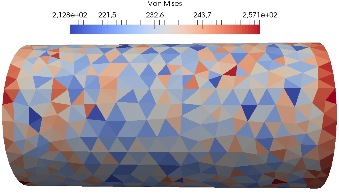
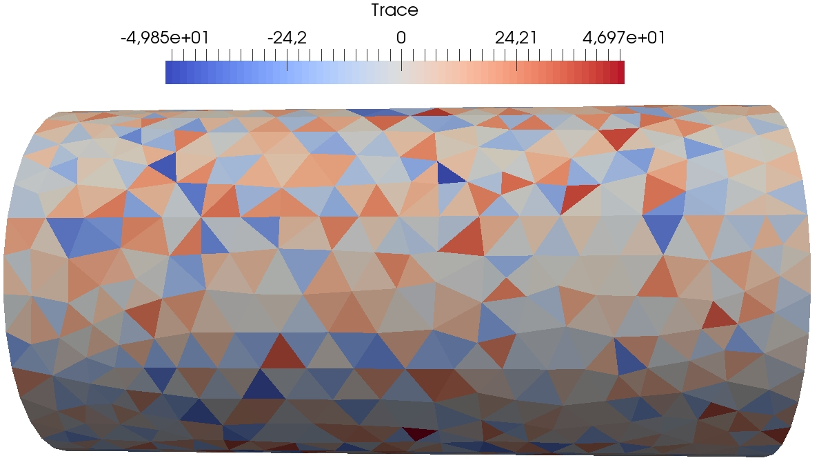
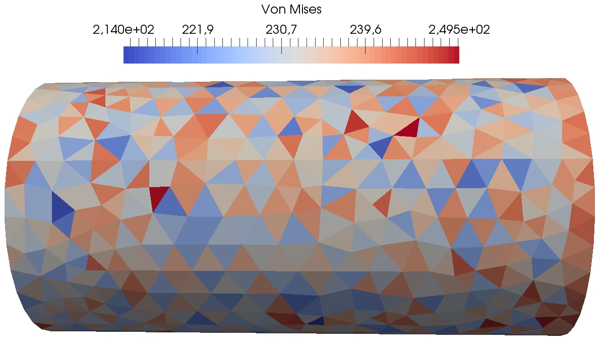
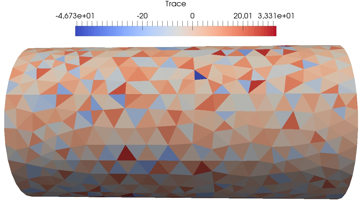
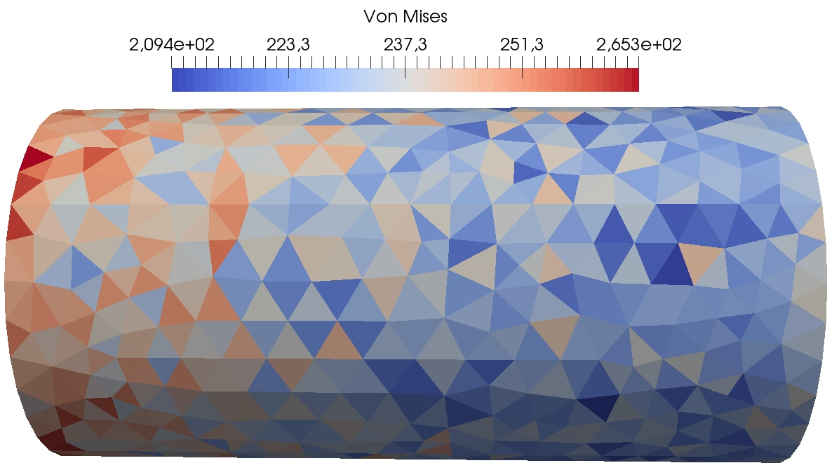
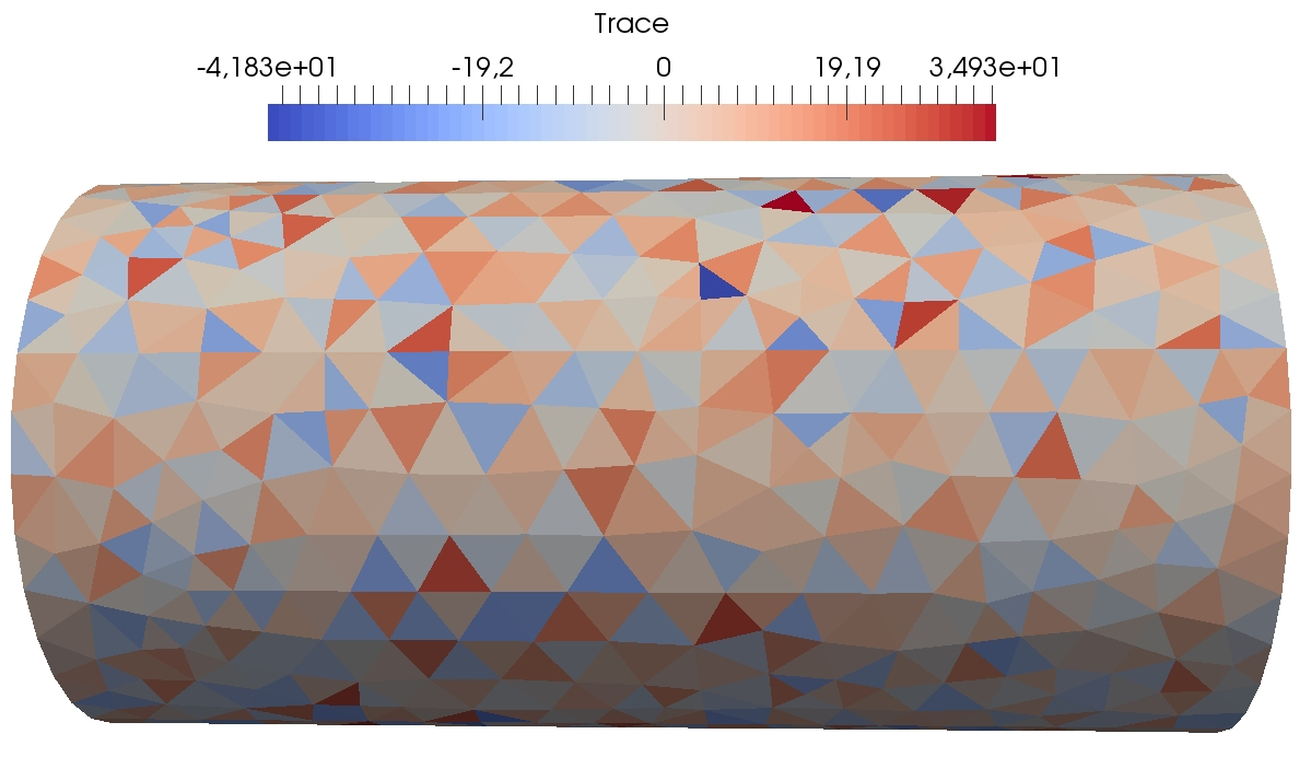
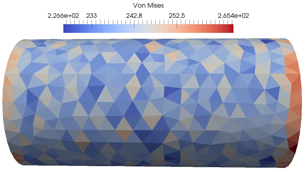
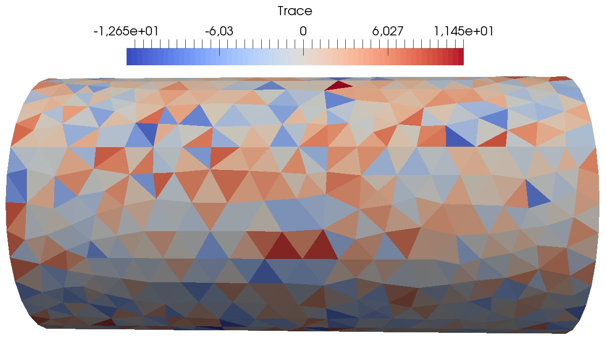
We observe that the influence of the parameter is rather light. Indeed, the trace of the trace tensor remains of order and the Von Mises stress varies between similar values. We observe that the results with the penalised Crouzeix–Raviart method vary slightly less. We believe that this is due to the higher number of dofs in this computation. As a consequence, so as to have a penalty term of the same order as the elastic term, we choose in our subsequent computations (unless explicitly mentioned).
3.5.2 Manufactured solution
Let us consider an isotropic two-dimensional elasticity test case in the domain with the Young modulus and the Poisson ratio . The reference solution is with and is the Cartesian basis of . The load term , which is computed accordingly, is , where and are the Lamé coefficients. The corresponding non-homogeneous Dirichlet boundary condition is enforced on the whole boundary. Convergence results are reported in Table 2 showing that the energy error converges to first-order with the mesh size and the -error to second-order.
| dofs | order | order | |||
|---|---|---|---|---|---|
| 0.0356 | 5.67942e-05 | - | 4.72e-03 | - | |
| 0.0177 | 8.62031e-06 | 2.76 | 1.50e-03 | 1.60 | |
| 0.00889 | 1.80278e-06 | 2.27 | 5.87e-04 | 1.55 |
4 Quasi-static elasto-plasticity
In this section we present the quasi-static elasto-plasticity problem, its DEM discretization, and we perform numerical tests to assess the methodology.
4.1 Governing equations
The quasi-static elasto-plastic problem is a simplified formulation of (9) where the inertia term in the mass bilinear form is negligible and where the time derivatives are substituted by discrete increments. Thus we consider a sequence of loads for all , and we consider the following sequence of nonlinear problems where for all :
| (39) |
where , , and where variables with a superscript n-1 come from the solution of the quasi-static problem (39) at the previous load increment or from a prescribed initial condition if . Given a quadruple , the procedure PLAS_IMP returns a quadruple such that
| (40) |
Moreover is the new stress tensor, and is the consistent elastoplastic modulus [23] such that
| (41) |
The consistent elastoplastic modulus is instrumental to solve (39) iteratively by using an implicit radial return mapping technique (close to Newton–Raphson iterations) [24]: Starting from , we solve iteratively the linear problem in such that
| (42) |
where the state for comes from the previous loading step or the initial condition. Convergence of the iterative process in is reached when the norm of the residual is small enough.
4.2 DEM space discretization
Using the DEM space discretization, the sequence of quasi-static problems (39) amounts to seeking a discrete triple for all , solving the following nonlinear problem:
| (43) |
where represents a suitable discretization of the load linear form . Using the radial return mapping technique as in (42) and starting from , we solve iteratively the linear problem in such that
| (44) |
with the residual , and where the discrete state for comes from the previous loading step or by interpolating the values of the initial condition at the cell barycentres and the boundary vertices. Convergence of the iterative process in is reached when the norm of the residual is small enough (we use a scaled Euclidean norm).
4.3 Numerical tests
This section contains two three-dimensional tests, a beam in quasi-static flexion and a beam in quasi-static torsion, and a two-dimensional test case on the swelling of an infinite cylinder with internal pressure.
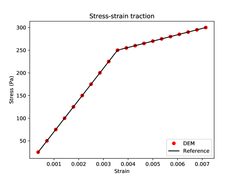
4.3.1 Beam in quasi-static traction
A beam of square section and is stretched by a displacement imposed at its right extremity, whereas the normal displacement and the tangential component of the normal stress are null at the left extremity. An homogeneous Neumann condition () is enforced on the four remaining sides of the beam. Figure 5 shows a sketch of the problem setup. The Young modulus is and the Poisson ratio . The yield stress is , and the material is supposed to be elasto-plastic with linear kinematic hardening. Specifically the tangent plastic modulus is set to , so that we have with . The imposed displacement is linearly increased in loading steps from to , where is the yield displacement. For this test case the analytical solution is available.
Figure 6 shows the stress-strain response curve, showing perfect agreement with the analytical solution using a mesh of size . Note that in this test case, the stress tensor is constant in the beam.
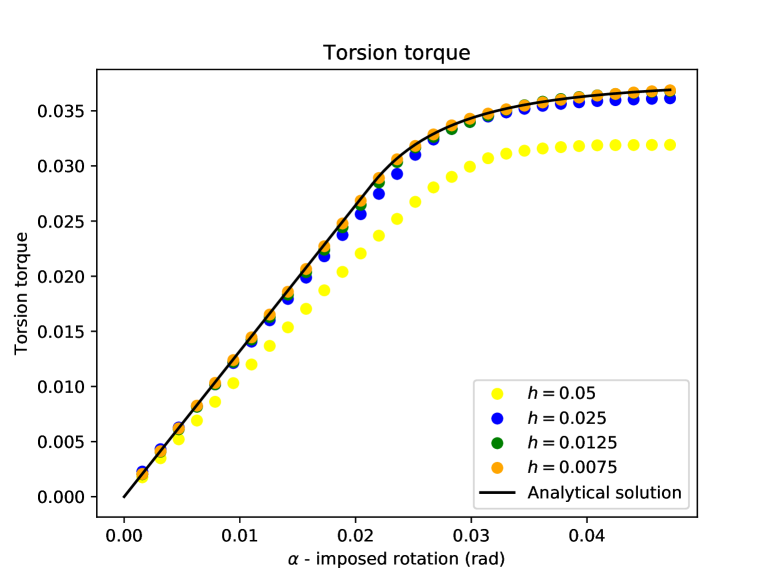
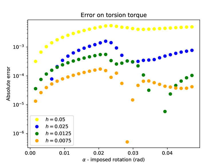
4.3.2 Beam in quasi-static torsion
A beam of length with a circular section of radius is subjected to torsion at one of its extremities. The Young modulus is and the Poisson ratio . The yield stress is , and the material is supposed to be perfectly plastic so that . The beam is clamped at one of its extremities, a torsion angle is imposed at the other extremity, and the rest of the boundary of the beam is stress free (). Figure 7 presents the problem setup. The torsion angle is increased linearly in 20 loading steps from to , where is the yield angle and is the second Lamé coefficient. An analytical solution is available in the cylindrical frame : the displacement field is , and the stress field is , where
Table 3 reports the maximum -error on the displacement (evaluated as in Section 3.5) over the simulation interval and the energy error (including the energy of the penalty terms). The errors are evaluated as described in Section 3.5. First-order convergence in the energy norm is observed, as expected. However, full second-order convergence in norm does not seem satisfied (although the convergence order is still above ). This can be due to the fact that in perfect plasticity which is a required hypothesis to obtain full second-order convergence.
| dofs | order | order | |||
| 2.62e-06 | - | 5.87e-04 | - | ||
| 1.02e-06 | 1.97e-04 | ||||
| 7.75e-07 | 1.53e-04 | ||||
| 4.50e-07 | 8.23e-05 | ||||
| 0.01418 | 2.14e-07 | 5.36e-05 |
Figure 8 presents the torque-angle response curve for the reference solution and the DEM solution on various meshes, showing good agreement and the convergence of the DEM predictions as the mesh is refined.
4.3.3 Inner swelling of an infinite cylinder
This test case consists in the inner swelling of an infinite cylinder. The inner radius is and the outer radius is . Owing to the symmetries, the computation is carried out on a quarter of a planar section of the cylinder with a plane strain formulation. A sketch of the problem setup is presented in Figure 9. On the lateral sides of the quarter of cylinder, a null normal displacement and a null tangential component of the normal stress are enforced. The outer side of the cylinder is stress free (), and the inner pressure imposed on the inner side is linearly increased from to , where is the initial yield stress. The Young modulus and the tangent plastic modulus are set to and .
Table 4 reports the -error on the displacement (evaluated as in Section 3.5) and on the cumulated plastic strain. The reference solution is computed on the finest mesh and is based on -Lagrange finite elements (FE) using the implementation available in [4]. The results in Table 4 show that the method converges at order two in the -norm and at order one in the energy norm.
| dofs | order | order | |||
|---|---|---|---|---|---|
| 0.07735 | 992 | 5.15e-4 | - | 3.05e-03 | - |
| 0.04217 | 3412 | 1.69e-4 | 8.38e-04 | ||
| 0.02879 | 7588 | 7.26e-5 | 3.76e-04 | ||
| 0.02172 | 13380 | 3.85e-5 | 2.10e-04 |
5 Space-time fully discrete elasto-plasticity
In this section we consider the dynamic elasto-plasticity equations from Section 2. The time discretization is performed by means of an explicit, pseudo-energy conserving, time-integration scheme recently introduced in [20]. The space discretization is achieved by means of the DEM scheme discussed in Sections 3 and 4. The main difference with Section 4.3 is that no iterative procedure is necessary in this section. Three-dimensional test cases are presented to assess the proposed methodology.
5.1 Time semi-discretization of dynamic elasto-plasticity
For simplicity we consider in this section only the time semi-discretization of the dynamic elasto-plasticity equations (9). We deal with the space-time fully discrete setting in the next section. The time-integration scheme [20] is a two-step method of order two which ensures a discrete pseudo-energy conservation, if the integration of forces is exact, even for nonlinear systems. Symmetric Gaussian quadratures of the forces can be used in practice as long as they are of order at least two. The time interval is discretized using the time nodes , and for simplicity we consider a constant time step . We define the half-time nodes for all . The time step is limited by a CFL condition which we specify in the fully discrete setting in the next section.
The key idea in the scheme [20] is to approximate the displacement field at the time nodes by means of functions , for all , with specified by the initial condition on the displacement, and the velocity field at the half-time nodes by means of functions , for all , with specified by the initial condition on the velocity. For all , given and , the scheme performs two substeps: (i) A time-dependent displacement field is predicted on the time interval using the free-flight expression for all ; (ii) The velocity field is predicted by means of a quadrature on the time-integration of the forces in the time interval . Let and be the nodes and the weights for the quadrature in the time interval . We then set
| (45) |
where is known from the free-flight displacement prediction and where the state for the first Gauss node comes from the previous time step or the initial condition. Given a triple , the procedure PLAS_EXP returns a pair such that, letting , we have
| (46) |
The main difference with respect to the procedure PLAS_IMP described in (40) is on the increment of the tensor of remanent plastic strain.
5.2 Space-time fully discrete scheme
Full space-time discretization is achieved by combining the time-integration scheme [20] described in the previous section with the DEM space discretization scheme from Section 3. For all , we compute a discrete displacement field and a discrete velocity field (recall that these spaces depend on if the prescribed Dirichlet condition on the displacement is time-dependent). Moreover, we compute a (trace-free) tensor of remanent plastic strain and a scalar cumulated plastic deformation for every mesh cell and every Gauss time-node . We set and . The fully discrete scheme reads as follows: For all , given , and , compute , , , and such that
| (47) |
where . Moreover, and are, respectively, the discrete mass bilinear form and the discrete load linear form. For the first Gauss node , the first two arguments in PLAS_EXP come from the previous time step or the initial condition. The initial displacement and the initial velocity are evaluated by using the values of the prescribed initial displacement and the prescribed initial velocity at the cell barycentres and the boundary vertices.
The time step is restricted by the following CFL stability condition:
| (48) |
where is the smallest entry of the diagonal mass matrix associated with the discrete mass bilinear form and is the largest eigenvalue of the stiffness matrix associated the discrete stiffness bilinear form (i.e., this maximal eigenvalue is computed in the worst-case scenario when there is no plasticity). The CFL condition (48) guarantees the stability of the time-integration scheme in the linear case [20], i.e., when there is no plasticity. We expect that this condition is still reasonable in the nonlinear case since plasticity does not increase the stiffness of the material.
Finally, let us write the discrete equivalent of the energy conservation property (11). Define the discrete elastic energy at as
with , for all . The discrete kinetic energy at is defined by
the discrete plastic dissipation at is defined by
and finally the work of external loads at is defined by
Then assuming a homogeneous Dirichlet condition for simplicity, we have the following energy balance equation:
| (49) |
where the term results from the use of quadratures to compute the integral of forces (recall that in our setting). The interested reader is referred to [20] for further details on the effect of quadratures on the conservation properties of the integration method.
5.3 Numerical tests
This section contains two three-dimensional test cases: a beam in dynamic flexion and a beam in dynamic torsion. We use the midpoint quadrature for the integration of the forces in each time step within the time-integration scheme. We refer the reader to [20] for a study of the influence of the quadrature on the scheme accuracy for various nonlinear problems with Hamiltonian dynamics.
Although the material parameters are indicated below using physical units, they are best interpreted in terms of characteristic times. For instance, considering a one-dimensional domain of length , the characteristic time of the numerical experiments is . The CFL condition (48) restricts the time-step as . Thus, one has
Since the ratio is independent of , the same conclusion holds for . Therefore we will report this time ratio in the computations.
5.3.1 Beam in dynamic flexion
This test case consists in computing the oscillations of an elastic and linearly isotropic plastic beam of length with a rectangular section of . The simulation time is . The beam is clamped at one end, it is loaded by a uniform vertical traction at the other end, and the four remaining lateral faces are stress free (). The load term is defined as
| (50) |
Figure 10 displays the problem setup. The material parameters are for the Young modulus, for the Poisson ratio, for the density, for the yield stress, and for the tangent plastic modulus. The present three-dimensional implementation used as a starting point [4], where -Lagrange FE and an implicit time-integration scheme are considered for a purely elastic material.
The proposed DEM is compared to penalised Crouzeix–Raviart FE [16]. This method is chosen as reference since it is known to be robust in the incompressible limit as . The penalty parameter is chosen as with . The reference computation is performed using vector-valued dofs and a time-step . Two computations are performed with the proposed DEM. The first uses a coarse mesh containing vector-valued dofs and a time-step , which is stable for the explicit integration. The second uses a fine mesh containg vector-valued dofs and a time-step , also stable for the explicit integration. Thus one has: . The penalty parameter for both computations is similar to the reference computation with . As already mentioned, we used a midpoint quadrature of the forces. Higher-order symmetric quadratures have been found to give overlapping results with respect to the midpoint quadrature. In all the computations, the time-discretization error is actually smaller than the space-discretization error, but larger time-steps cannot be considered owing to the CFL restriction.
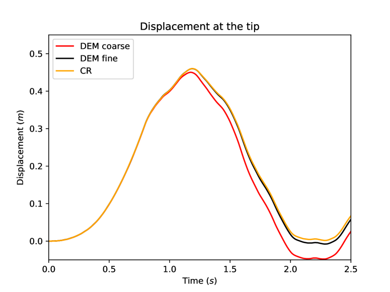
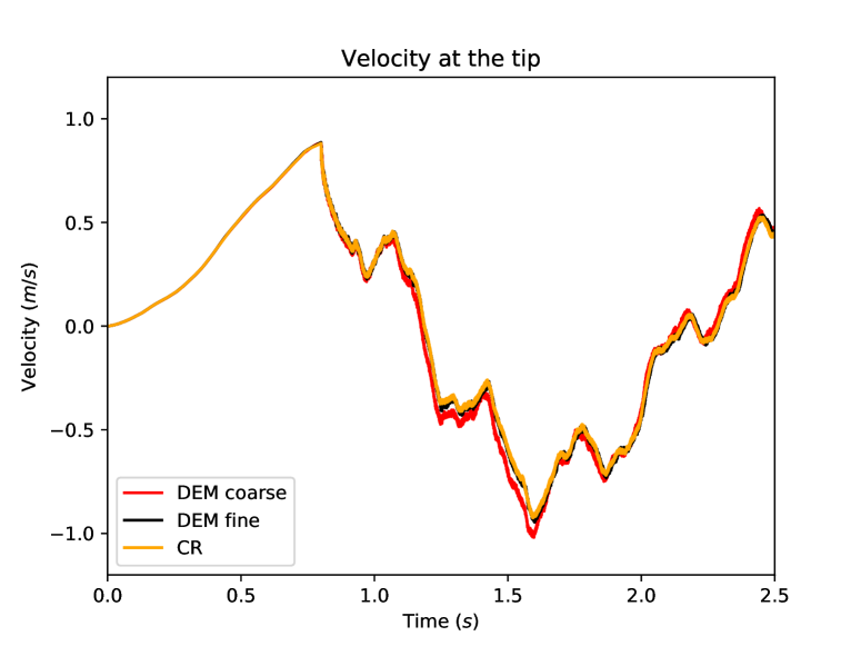
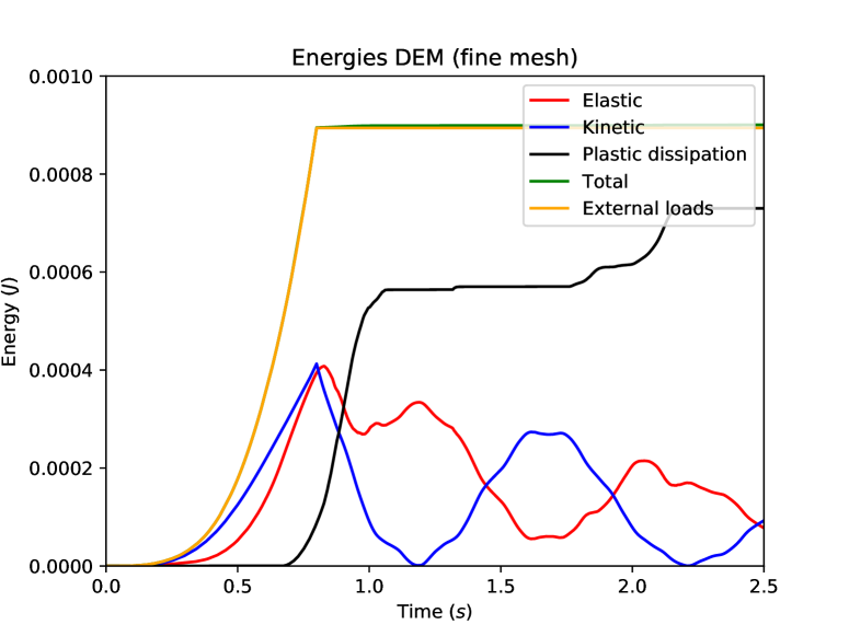
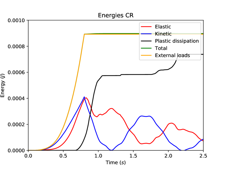
The displacement and the velocity at the center of the loaded tip of the beam are compared in Figure 11. We notice the excellent agreement between the DEM prediction on the fine mesh and the reference computation. Figure 12 shows the balance of energies for the reference computation and the fine DEM computation. One can first notice that the total energy for both DEM and Crouzeix–Raviart space semi-discretizations is well preserved by the time-integrator [20] since the total mechanical energy (kinetic energy, elastic energy and plastic dissipation) and the work of the external load are perfectly balanced at all times. We also notice that the amount of plastic dissipation is rather significant at the end of the simulation.
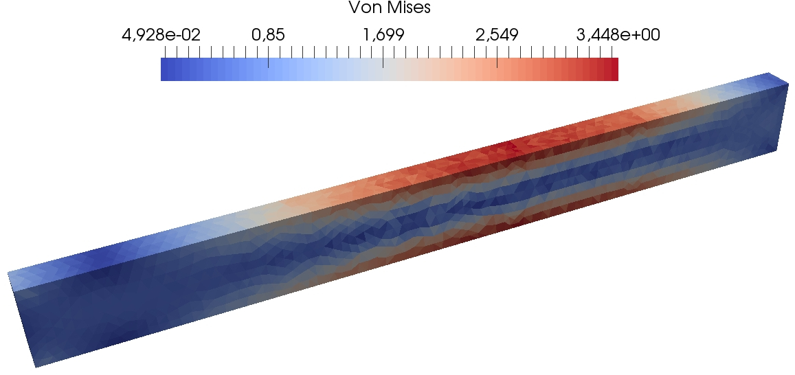
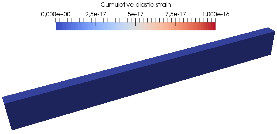
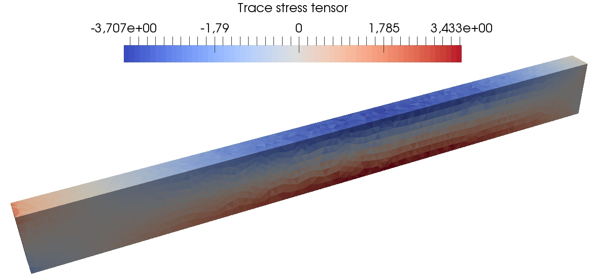
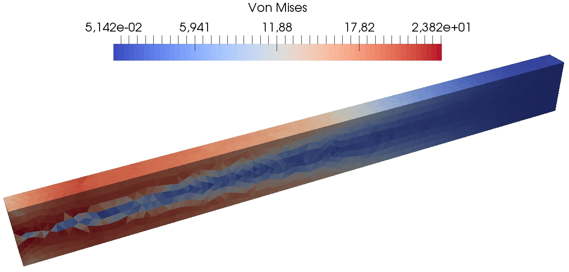
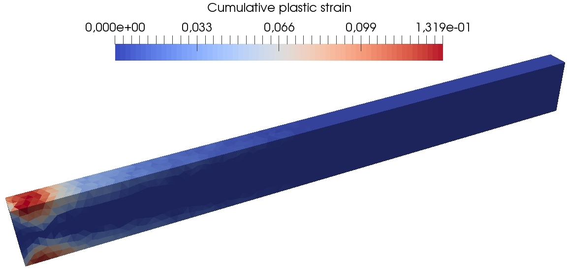
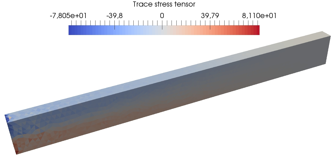
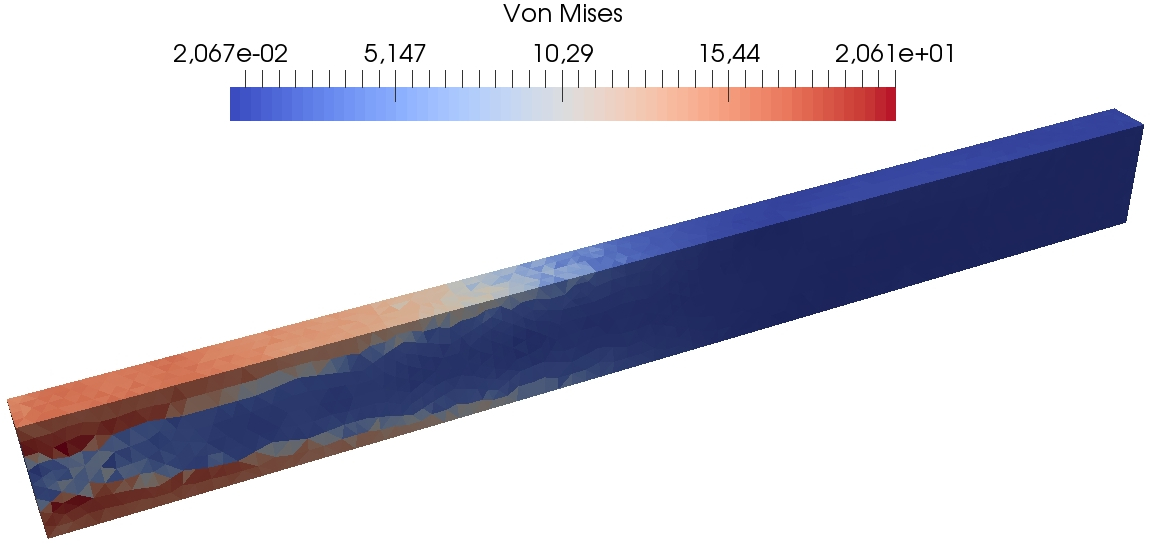

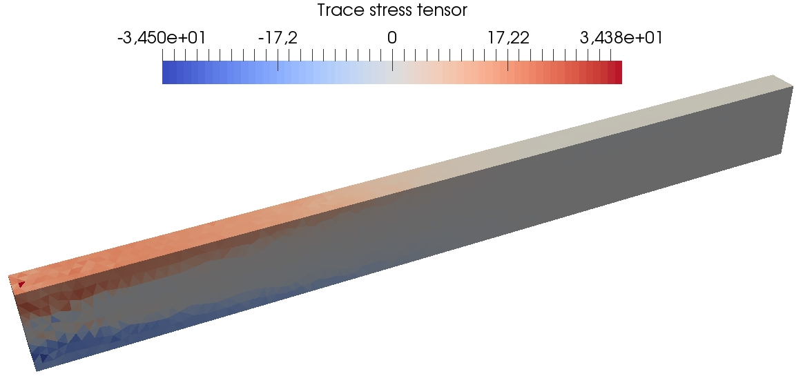
Figure 13 presents some further results of the DEM computations on the fine mesh so as to visualize at three different times during the simulation the spatial localization of the von Mises equivalent stress, the cumulated plastic strain, and the trace of the stress tensor. One can see that the plastic strain is concentrated close to the clamped tip of the beam, where the material undergoes the greatest stresses. The method does not exhibit any locking due to plastic incompressibility as indicated by the smooth behavior of the trace of the stress tensor.
5.3.2 Beam in dynamic torsion
The setting is similar to the quasi-static torsion test case presented in Section 4.3.2. The two differences are the material parameters and the plastic law which are similar to Section 5.3.1, and the boundary conditions on one side of the beam. Figure 14 shows the problem setup. On one of its extremities the beam is clamped, and on the other extremity the following normal stress is imposed:
| (51) |
where and are defined in Section 4.3.2. The angle is increased from at to at , where is the yield angle defined in Section 4.3.2. The plastic parameters are the same as those in Section 5.3.1.
Three different space discretizations are considered for this test case: -Lagrange FE, penalised Crouzeix–Raviart FE and the proposed DEM. The Crouzeix–Raviart computations are used as reference since the method is known to be robust with respect to the incompressible limit. The Lagrange FE computations are used to illustrate their inability to deal with large plastic (deviatoric) strains. The goal of this test case is to show the ability of the proposed DEM to deal with deviatoric plasticity. The computations are not performed on the same meshes but rather with meshes leading to a similar number of dofs so as to give comparable results for DEM and Lagrange FE, whereas the meshes used with penalised Crouzeix–Raviart FE lead to twice as many dofs since they are employed to obtain a reference solution. The number of dofs and the time-steps used in the computations are presented in Table 5.
| Method | DEM | Lagrange FE | penalised CR FE | |||
|---|---|---|---|---|---|---|
| Computation | coarse | fine | coarse | fine | fine | very fine |
| Vectorial dofs | ||||||
One thus has: . All the reported time-steps are compatible with the CFL restriction. Also, for all computations, we have verified that the time discretization error is negligible with respect to the space discretization error. The time-integration scheme [20] is used with a midpoint quadrature of the forces for the coarse computations and with a Gauss-Legendre quadrature of the forces of order 5 for the fine computations. For details on the effect of the quadrature rule, see [20].
The comparison between the methods is performed by considering the displacement and the velocity of the point of coordinates over the simulation time . The results are reported in Figure 15.
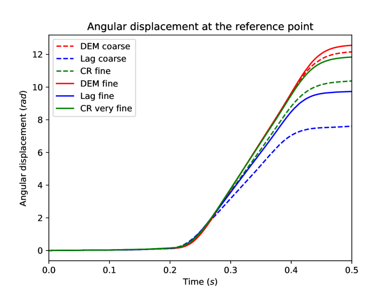
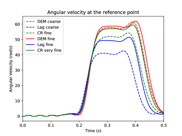
The angular velocity plot indicates for times s the presence of elastic waves with a small magnitude travelling through the beam. The wave of larger amplitude arriving afterwards is a plastic wave whose velocity is ten times smaller than the elastic waves since . We notice that the value for the simulation time is too long for the simulation to remain physically relevant within the small strain assumption owing to the large value reached by the angular displacement of the reference point. However this setting allows us to reach substantial amounts of plastic dissipation and thereby to probe the robustness of the space semi-discretization methods with respect to incompressibility. Recall that the remanent plastic strain tensor is trace-free, so that the stress tensor is nearly deviatoric in the entire beam at the end of the simulation. Such a situation is challenging for the -Lagrange FEM since this method is known to lock in the incompressible limit. To highlight the volumetric locking incurred by Lagrange FE, Figure 16 displays at the time the trace of the stress tensor predicted by Lagrange FE (fine mesh) and penalised Crouzeix–Raviart FE (coarse mesh), for a similar number of dofs.
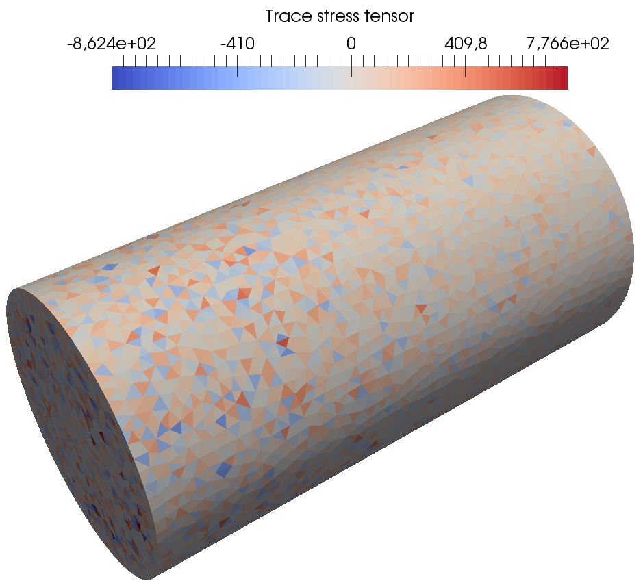
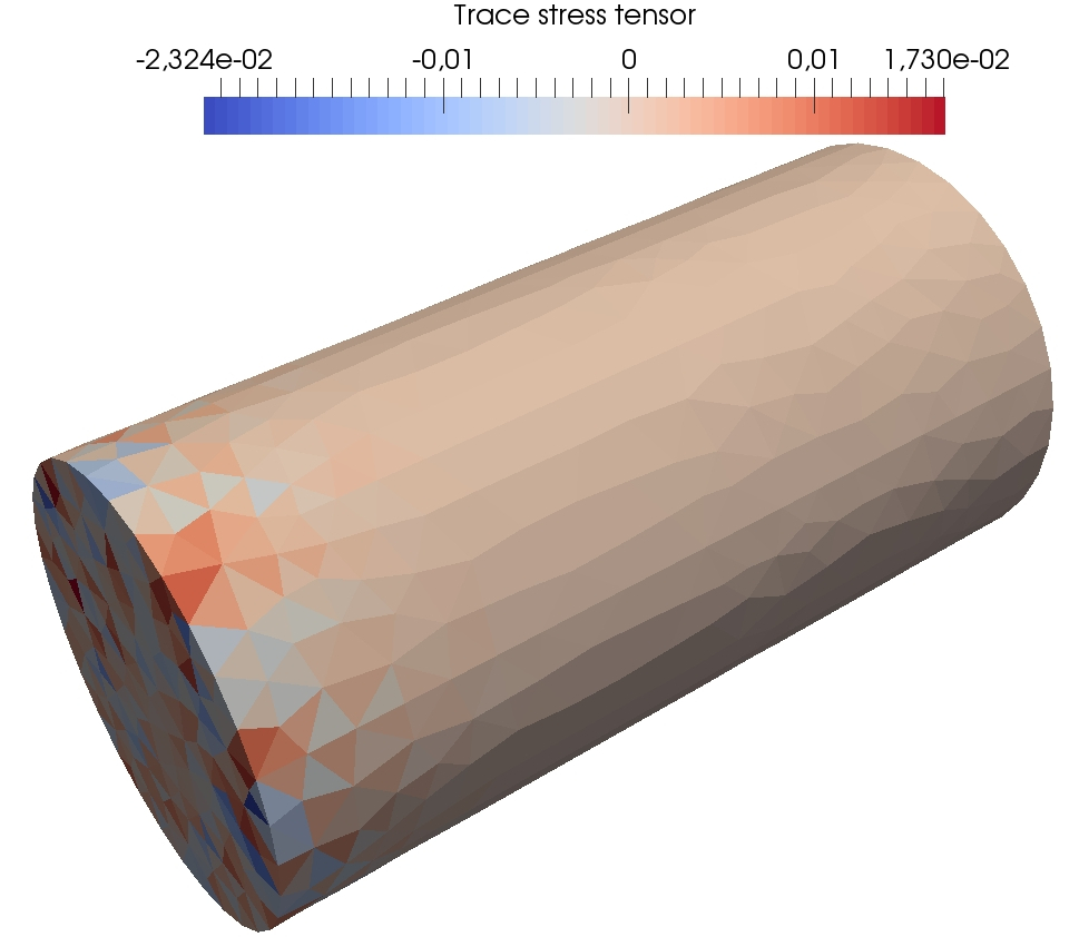
For Lagrange FE, significant oscillations are visible in the whole beam (the amplitude of these oscillations is about ten times the maximal value of the von Mises equivalent stress). Also, the amplitudes of the oscilliations of the trace tensor are about four times larger than for penalised Crouzeix–Raviart FE. Figure 17 reports the energies on the fine meshes for the DEM, Lagrange FE and penalised Crouzeix–Raviart FE. First, we notice as in the previous test case the prefect balance of the work of external loads with the different components of the mechanical energy. The orders of magnitude of the energies and plastic dissipations are similar for the three methods. However, a significant discrepancy in the plastic dissipation can be observed for Lagrange FE with respect to penalised Crouzeix–Raviart FE and DEM which both give a plastic dissipation similar to the reference computation.
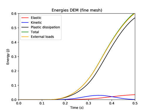
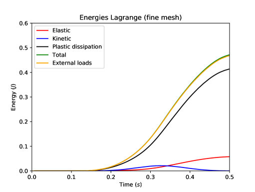
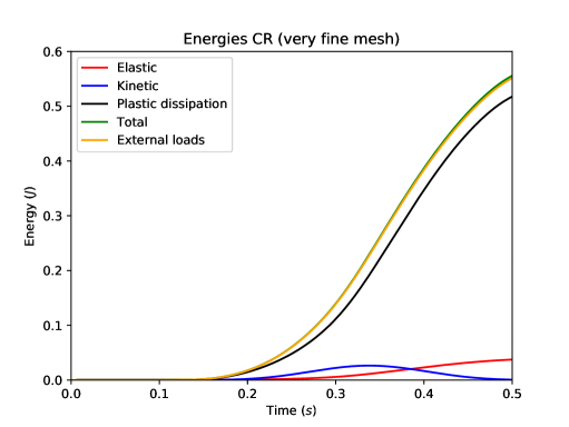
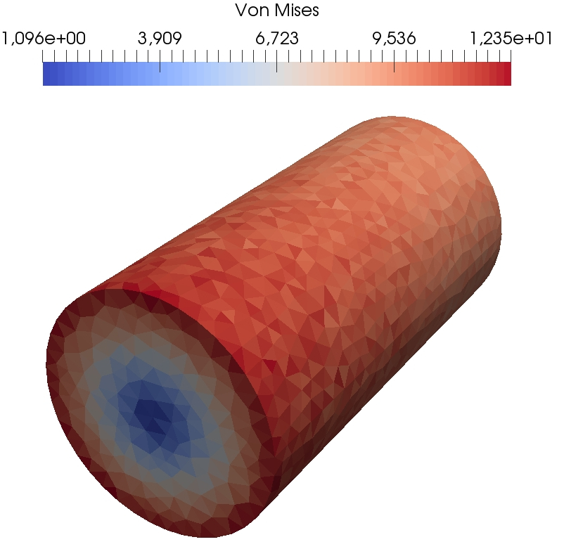
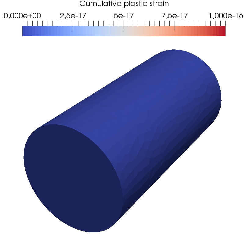
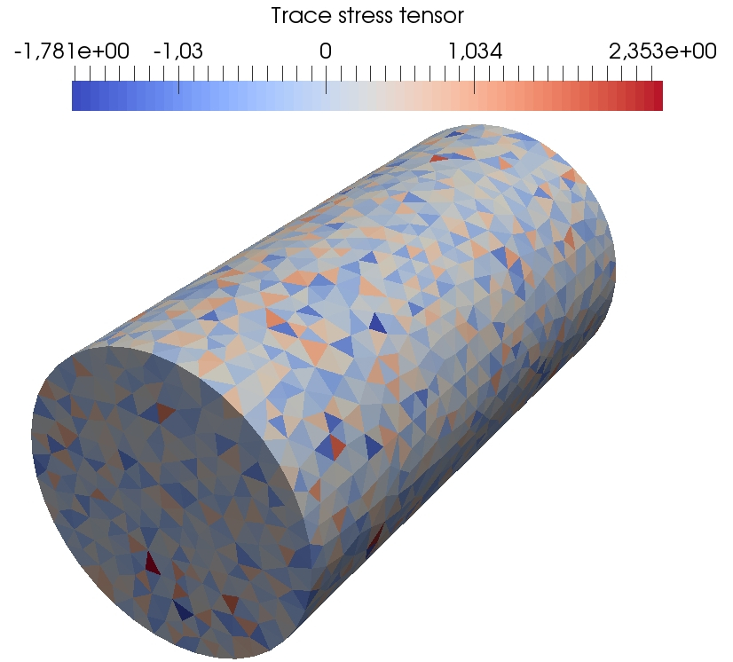
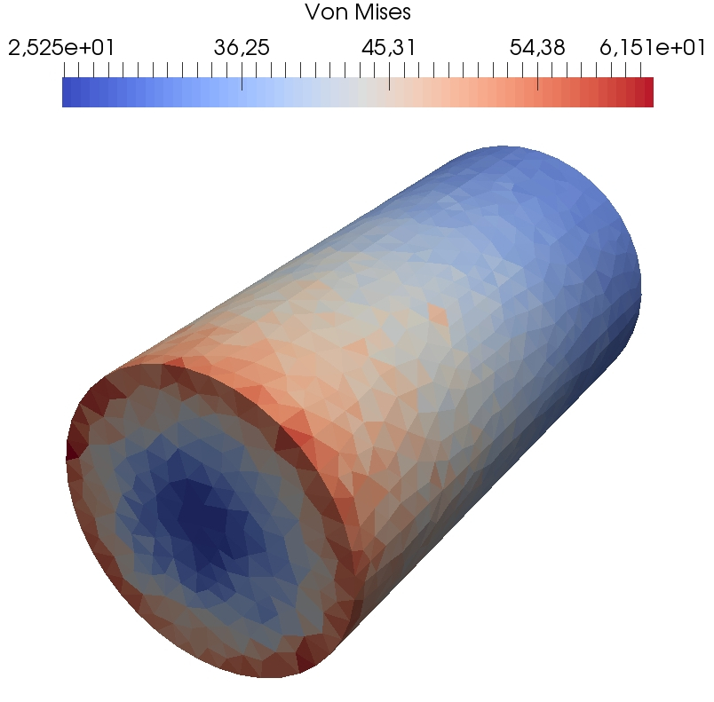
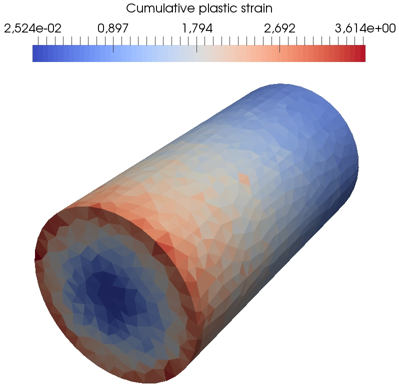
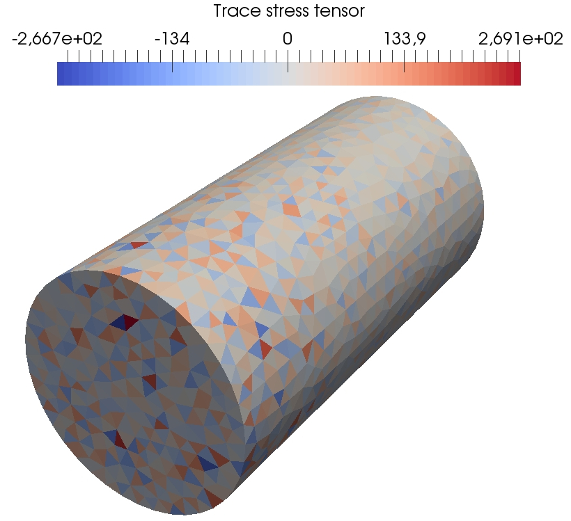

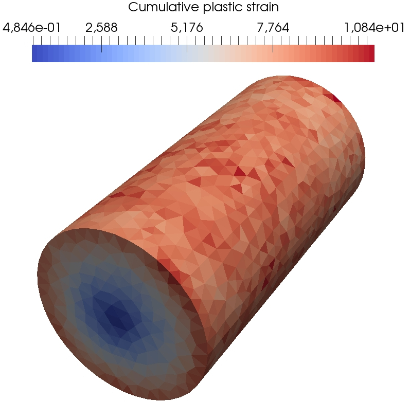
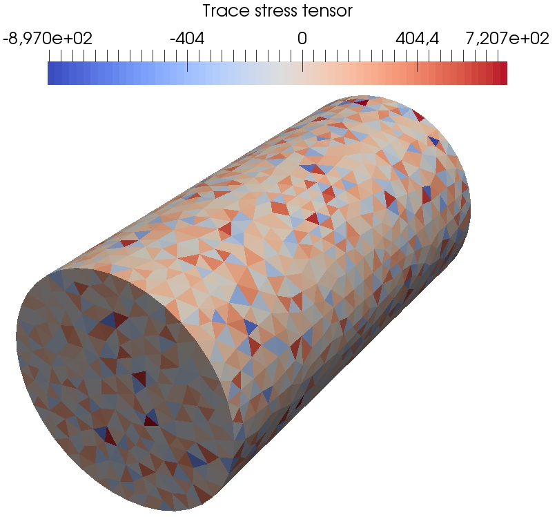
Figure 18 presents some further results of the DEM computations on the fine mesh so as to visualize at three different times during the simulation the spatial localization of the von Mises equivalent stress, the cumulated plastic strain, and the trace of the stress tensor. We can see in the first row that the von Mises stress is nonzero in the entire beam and thus the elastic waves have already travelled through the entire beam whereas the cumulative plastic strain is still zero and thus no plastic flow has occurred. In the second row, we can see that a plastic wave has started to propagate from one end of the beam. In the last row, we see that the plastic wave has reached the other side of the beam at the end of the simulation. Also, regarding the robustness with respect to , the magnitude of the oscillations of the trace of the stress tensor is similar to penalised Crouzeix–Raviart FE. Indeed for the DEM, the extreme values of the trace of the stress tensor are and at and and at whereas for penalised Crouzeix–Raviart FE the extermes values are and at and and at . Comparatively, for the -Lagrange FE computations, the extreme values of the trace of the stress tensor are and for and and for .
6 Conclusion
We have presented a new Discrete Element Method which is a variational discretization of a Cauchy continuum and which only requires continuum macroscopic parameters as the Young modulus and the Poisson ratio for its implementation. The displacement degrees of freedom are attached to the barycentres of the mesh cells and to the boundary vertices. The key idea is to reconstruct displacements on the mesh facets and then to use a discrete Stokes formula to devise a piecewise constant gradient and linearized strain reconstructions. A simple geometric pre-processing has been devised to ensure that for almost all the mesh facets, the reconstruction is based on an interpolation (rather than extrapolation) formula and we have shown by numerical experiments that this choice can produce highly beneficial effects in terms of the largest eigenvalue of the stiffness matrix, and thus on the time step restriction within explicit time-marching schemes. Moreover, in the case of elasto-plastic behavior, the internal variables for plasticity are piecewise-constant in the mesh cells. The scheme has been tested on quasi-static and dynamic test cases using a second-order, explicit, energy-conserving time-marching scheme. Future work can include adapting the present framework to dynamic cracking and fragmentation as well as to Cosserat continua. An extension to large strain solid dynamics could also be performed by working in the reference configuration.
Acknowledgements
The authors would like to thank K. Sab (Navier, ENPC) and J.-P. Braeunig and L. Aubry (CEA) for fruitful discussions. The authors would also like to thank J. Bleyer (Navier, ENPC) for his help in dealing with the Fenics implementations. The PhD fellowship of the first author was supported by CEA.
Conflict of interest
The authors declare no conflict of interest.
References
- [1] D. André, J. Girardot, and C. Hubert. A novel DEM approach for modeling brittle elastic media based on distinct lattice spring model. Computer Methods in Applied Mechanics and Engineering, 350:100–122, 2019.
- [2] D. André, M. J., I. Iordanoff, J.-L. Charles, and J. Néauport. Using the discrete element method to simulate brittle fracture in the indentation of a silica glass with a blunt indenter. Computer Methods in Applied Mechanics and Engineering, 265:136–147, 2013.
- [3] D. Arnold. An interior penalty finite element method with discontinuous elements. SIAM journal on numerical analysis, 19(4):742–760, 1982.
- [4] J. Bleyer. Numerical tours of computational mechanics with FEniCS, 2018. https://zenodo.org/record/1287832#.Xbsqdvco85k.
- [5] M. Budninskiy, B. Liu, Y. Tong, and M. Desbrun. Power coordinates: a geometric construction of barycentric coordinates on convex polytopes. ACM Transactions on Graphics (TOG), 35(6):241, 2016.
- [6] C. Carstensen. Numerical analysis of the primal problem of elastoplasticity with hardening. Numerische Mathematik, 82(4):577–597, 1999.
- [7] M. A. Celigueta, S. Latorre, F. Arrufat, and E. Oñate. Accurate modelling of the elastic behavior of a continuum with the discrete element method. Comput. Mech., 60(6):997–1010, 2017.
- [8] P. Cundall and O. Strack. A discrete numerical model for granular assemblies. geotechnique, 29(1):47–65, 1979.
- [9] D. A. Di Pietro. Cell centered Galerkin methods for diffusive problems. ESAIM: Mathematical Modelling and Numerical Analysis, 46(1):111–144, 2012.
- [10] D. A. Di Pietro and A. Ern. Mathematical aspects of discontinuous Galerkin methods, volume 69. Springer Science & Business Media, 2011.
- [11] J. Droniou, R. Eymard, T. Gallouët, C. Guichard, and R. Herbin. The gradient discretisation method, volume 82. Springer, 2018.
- [12] R. Eymard, T. Gallouët, and R. Herbin. A finite volume scheme for anisotropic diffusion problems. Comptes Rendus Mathématique, 339(4):299–302, 2004.
- [13] R. Eymard, T. Gallouët, and R. Herbin. Discretization of heterogeneous and anisotropic diffusion problems on general nonconforming meshes SUSHI: a scheme using stabilization and hybrid interfaces. IMA Journal of Numerical Analysis, 30(4):1009–1043, 2009.
- [14] W. Han and X. Meng. Error analysis of the reproducing kernel particle method. Comput. Methods Appl. Mech. Engrg., 190(46-47):6157–6181, 2001.
- [15] W. Han and B. D. Reddy. Plasticity: mathematical theory and numerical analysis, volume 9. Springer Science & Business Media, 2012.
- [16] P. Hansbo and M. Larson. Discontinuous galerkin and the crouzeix–raviart element: application to elasticity. ESAIM: Mathematical Modelling and Numerical Analysis, 37(1):63–72, 2003.
- [17] W.G. Hoover, W.T. Ashurst, and R.J. Olness. Two-dimensional computer studies of crystal stability and fluid viscosity. The Journal of Chemical Physics, 60(10):4043–4047, 1974.
- [18] M. Jebahi, D. André, I. Terreros, and I. Iordanoff. Discrete element method to model 3D continuous materials. John Wiley & Sons, 2015.
- [19] C. Labra and E. Oñate. High-density sphere packing for discrete element method simulations. Comm. Numer. Methods Engrg., 25(7):837–849, 2009.
- [20] F. Marazzato, A. Ern, C. Mariotti, and L. Monasse. An explicit pseudo-energy conserving time-integration scheme for hamiltonian dynamics. Comput. Methods Appl. Mech. Engrg., 347:906 – 927, 2019.
- [21] L. Monasse and C. Mariotti. An energy-preserving Discrete Element Method for elastodynamics. ESAIM: Mathematical Modelling and Numerical Analysis, 46:1527–1553, 2012.
- [22] H. Nilsen, I. Larsen, and X. Raynaud. Combining the modified discrete element method with the virtual element method for fracturing of porous media. Comput. Geosci., 21(5-6):1059–1073, 2017.
- [23] J. C. Simo and R. L. Taylor. Consistent tangent operators for rate-independent elastoplasticity. Computer methods in applied mechanics and engineering, 48(1):101–118, 1985.
- [24] N. Q. Son. On the elastic plastic initial-boundary value problem and its numerical integration. International Journal for Numerical Methods in Engineering, 11(5):817–832, 1977.
- [25] M. Spellings, R. L. Marson, J. A. Anderson, and S. C. Glotzer. GPU accelerated discrete element method (DEM) molecular dynamics for conservative, faceted particle simulations. J. Comput. Phys., 334:460–467, 2017.