A wall model based on neural networks for LES of turbulent flows over periodic hills
Abstract
In this work, a data-driven wall model for turbulent flows over periodic hills is developed using the feedforward neural network (FNN) and wall-resolved LES (WRLES) data. To develop a wall model applicable to different flow regimes, the flow data in the near wall region at all streamwise locations are grouped together as the training dataset. In the developed FNN wall models, we employ the wall-normal distance, near-wall velocities and pressure gradients as input features and the wall shear stresses as output labels, respectively. The prediction accuracy and generalization capacity of the trained FNN wall model are examined by comparing the predicted wall shear stresses with the WRLES data. For the instantaneous wall shear stress, the FNN predictions show an overall good agreement with the WRLES data with some discrepancies observed at locations near the crest of the hill. The correlation coefficients between the FNN predictions and WRLES predictions are larger than 0.7 at most streamwise locations. For the mean wall shear stress, the FNN predictions agree very well with WRLES data. More importantly, overall good performance of the FNN wall model is observed for different Reynolds numbers, demonstrating its good generalization capacity.
I Introduction
Separation and reattachment in turbulent flows over curved surfaces exist in numerous environmental and industrial processes, e.g. underwater vehicle, fuselages at high incidence, curved ducts, and stalled wings and turbine blades. Such flows are difficult to predict accurately using Reynolds-Averaged Navier-Stokes (RANS) method due to non-equilibrium spatial and temporal fluctuations, although it is widely used in engineering applications. On the other hand, large-eddy simulation, which directly solve energetic turbulence scales and model the subgrid scales, being significantly less computational expensive than direct numerical simulation (DNS) Moin and Mahesh (1998); Choi and Moin (2012); He et al. (2017), provides a feasible way for simulating complex turbulent flows with separation and reattachment at a reasonable cost. However, it is still not applicable to employ wall-resolved large-eddy simulation (WRLES) in the design and optimization of high Reynolds number turbulent flow problems in real life because of the extremely high resolution needed to resolve the viscous scale near the wall Piomelli and Balaras (2002); Choi and Moin (2012). To reduce the computational cost of WRLES, wall models are employed in the literature Cabot and Moin (2000); Davidson (2009) to avoid the need to resolve the small scale turbulence in the near wall region, providing a feasible way for LES of wall-bounded flows at high Reynolds number. However, most existing wall models Piomelli (2008); Bose and Park (2018) based on equilibrium hypothesis are incapable of predicting flow separations and reattachments. The development of machine learning methods Duraisamy et al. (2019); Brunton et al. (2020) and the availability of high-resolution data from experiments and high-fidelity simulations provide another possible approach for developing advanced wall models for complex turbulent flows. As the first step, in this work we develop the wall models based on neural networks for turbulent flows over periodic hills.
We first briefly review different wall models developed in the literature. In wall-modeled LES, the turbulent flow near the wall is described by a wall-layer model with its influence on the outer flow represented by appropriate boundary conditions. The wall-stress model is the most widely used one in the literature, in which the wall shear stress is computed and provided as boundary conditions for outer flow simulations. Different models have been developed in the literature for computing wall shear stress, which include the equilibrium-stress model and zonal model (also dubbed as two-layer model) Bose and Park (2018). The algebraic equilibrium-stress models assume a constant-stress layer near the wall Pope (2000) and calculate the wall shear stress using the law of the wall of deterministic form Piomelli (2008). The algebraic model has the advantage of low computational cost, but it cannot accurately predict the wall shear stress in non-equilibrium flows, for which the equilibrium-stress hypothesis is no longer valid. The zonal model, on the other hand, solves the thin-boundary-layer equation (TBLE) on an embedded grid between the first grid point and the wall. Wang and Moin Wang and Moin (2002) systematically studied the efficacy of zonal models and found that the instantaneous wall shear stress cannot be accurately predicted when the non-equilibrium terms are ignored or the pressure gradient term is only considered. Later, the dynamic zonal models were proposed, which adjust mixing-length eddy viscosity in TBLE, and shown being able to predict low-order turbulence statistics Kawai and Larsson (2013); Park and Moin (2014). The integral wall model was also developed in the literature Yang et al. (2015a), which introduces an additional linear term into the equilibrium logarithmic velocity profile and accounts for near-wall non-equilibrium effects by solving the vertically integrated momentum equation. However, this model has only been tested in applications in which the non-equilibrium effects is insignificant. Besides the wall-stress type models, the virtual-wall model was also developed by aligning the slip velocity in the integrated TBLE on the virtual wall Chung and Pullin (2009); Cheng et al. (2015). It has been demonstrated being capable of capturing the quantitative features of a separation-reattachment turbulent boundary-layer flow at low to moderately large Reynolds numbers. However, the identification of virtual wall in a virtual-wall model is challenging for flows with complex geometries. Recently, the dynamic slip wall model was developed Bose and Moin (2014); Bae et al. (2018) to model the wall shear stress from the derivation of the LES equations using a differential filter, but its accuracy is sensitive to the subgrid-scale (SGS) models and numerical methods. The conventional wall models have been applied to different kinds of flows Larsson et al. (2016); Frere et al. (2018); Bose and Park (2018); Bae et al. (2019), but they still cannot accurately predict the flow separation and reattachment. Advanced wall model accounting for such non-equilibrium effects is still yet to develop.
Thanks to the exponetial growth in computing power, the increasing amount of high-fidelity data provides a possibility to develop data-driven wall models to resolve the above issues. The data-based approches, particularly the machine learning (ML) method, have been applied to various turbulence problems, e.g. the development of turbulence models Ling et al. (2016a); Zhou et al. (2019), temporal prediction of turbulence King et al. (2018); Lee and You (2019), and reconstruction of the turbulent flow fields Fukami et al. (2019); Liu et al. (2020). For the applications of the ML method in developing RANS models, Ling et al. Ling et al. (2016a) presented a deep neural network for RANS turbulence modeling on an invariant tensor basis Ling et al. (2016b). Xiao and co-workers Wang et al. (2017); Wu et al. (2018) developed a physics-informed ML framework to learn Reynolds stress discrepancies between RANS and DNS. Duraisamy et al. Duraisamy et al. (2019) reviewed in detail the recent developments of RANS turbulence models based on ML. As for LES models, the ML has been applied to model the SGS stresses in different flows including the turbulent channel flows Gamahara and Hattori (2017), two-dimensional decaying turbulence Maulik et al. (2018) and isotropic turbulence Zhou et al. (2019), and to model the SGS scalar flux Vollant et al. (2017). For the wall-bounded turbulent flows, the ML was also employed to develop wall models Milano and Koumoutsakos (2002), which is the major concern of this work. Recently, Yang et al. Yang et al. (2019) developed a wall-stress model for LES of turbulent channel flow using DNS data and physics-informed neural networks. They found that the trained wall model outperforms the conventional equilibrium wall model in simulating the three-dimensional boundary-layer flow. A simliar neural network was then applied to spanwise rotating turbulent channel flows with a discussion on the performance of physics-based and data-based approaches Huang et al. (2019). However, to the best of our knowledge, the non-equilibrium effects, e.g. pressure gradients, curvature and separation, which are important for complex turbulent flows in engineering applications, have not been taken into account in the existing data-driven wall model and need to be systematically investigated.
Characteristics of complex wall-bounded turbulent flows depends on the geometry of the boundary and the corresponding boundary conditions. Development of a wall model applicable to different turbulent flows does not seem feasible or at least beyond the scope of this work. The flow over periodic hills, in which the flow is featured by separation from a curved surface, recirculation, reattachment and strong pressure gradient, is an ideal generic test case for developing statistical closures for separated flow Fröhlich et al. (2005). Different wall models have been applied to simulate the flow over periodic hills. For instance, Temmerman et al. Temmerman et al. (2003) applied the equilibrium wall models to simulate the flow over periodic hills, and found that the sensitivity of the solution to the SGS model is lower than that to grid resolution and wall model. Furthermore, they demonstrated that the WMLES cannot accurately predict the flow separation, reattachment and related statistics. To simulate the flow over periodic hills, Manhart et al. Manhart et al. (2008) proposed an extended inner scaling for the wall layer of wall-bounded flows under the influence of both wall shear stress and adverse pressure gradient. Duprat et al. Duprat et al. (2011) constructed a new wall model based on the simplified TBLE, which takes into account both the streamwise pressure gradient and the Reynolds stresses effects, and applied it to simulate the flow over periodic hills. It was shown that their proposed model yields good results for predictions of first order statistics and reproduction of flow separation. To investigate in detail the separation and reattachment process, Breuer et al. Breuer et al. (2009) carried out numerical and wind tunnel experiment of the flow over periodic hills at various Reynolds numbers in the range of 100 to 10595. Rapp and Manhart Rapp and Manhart (2011) experimentally investigated the flow over periodic hills at four Reynolds numbers ranging from 5600 to 37000. Krank et al. Krank et al. (2018) carried out DNS of the flow over periodic hills at Reynolds number 10595, which is the highest fidelity to date. Moreover, Xiao et al. Xiao et al. (2020) constructed benchmark datasets for the flow over periodic hills by performing DNS with varing flow configurations to alleviate the lack of data for training and testing data-driven models.
The objective of this work is to develop a data-driven wall model for the flow over periodic hills using the feedforward neural network (FNN) and WRLES data. The datasets employed for training the model consist of flow field data in the near-wall flow region at all streamwise locations with different flow features. To train the FNN wall model, we employ the wall-normal distance, near-wall velocities and pressure gradients as input features and the wall shear stresses as output labels, respectively. The trained wall model is evaluated using the data from different snapshots and spanwise slices for both training and testing datasets.
The rest of the paper is organized as follows: In Section II, WRLES of the flow over periodic hills is briefly described, which is followed by the procedure for preparing datasets for training and testing FNN models. The feedforward neural network is introduced and trained in Section III. Then, the evaluation of the trained wall model is presented in Section IV. At last, conclusions from this work are drawn in Section V.
II Data generation and preparation
II.1 Data generation using wall-resolved large-eddy simulation
In this section, we describe the numerical method and the case setup for generating the data employed for developing a data-driven wall model, which can take into account the non-equilibrium effects, e.g. flow separation and reattachment, for turbulent flows over periodic hills.
We employ the Virtual Flow Simulator (VFS-Wind) Yang et al. (2015b); Yang and Sotiropoulos (2018) code for WRLES of turbulent flows over periodic hills. The VFS code has been successfully applied to industrial and environmental turbulent flows Kang and Sotiropoulos (2012); Kang et al. (2014); Khosronejad and Sotiropoulos (2014); Yang et al. (2017a); Yang and Sotiropoulos (2019a, b); Foti et al. (2019); Khosronejad et al. (2020). In VFS-Wind code, the governing equations are the three-dimensional unsteady spatially filtered incompressible Navier-Stokes equations in non-orthogonal, generalized curvilinear coordinates shown as follows:
| (1) | ||||
where and are the Cartesian and curvilinear coordinates, respectively, are the transformation metrics, is the Jacobian of the geometric transformation, is the -th component of the velocity vector in Cartesian coordinates, is the contravariant volume flux, are the components of the contravariant metric tensor, is the fluid density, is the dynamic viscosity, and is the pressure. In the momentum equation, represents the anisotropic part of the subgrid-scale stress tensor, which is modeled by the dynamic eddy viscosity subgrid-scale model,
| (2) |
where is the filtered strain-rate tensor and is the eddy viscosity calculated by
| (3) |
where is the model coefficient calculated dynamically using the procedure of Germano et al. Germano et al. (1991), and is the filter size, where is the cell volume.
The governing equations are spatially discretized using a second-order accurate central differencing scheme, and integrated in time using the fractional step method. An algebraic multigrid acceleration along with generalized minimal residual method (GMRES) solver is used to solve the pressure Poisson equation. A matrix-free Newton-Krylov method is used for solving the discretized momentum equation. More details about the flow solver can be found in the referencesGe and Sotiropoulos (2007); Kang et al. (2011); Yang et al. (2015b).
The geometry of the periodic hills is shown in Figure 1, which has been extensively employed in experiments Breuer et al. (2009); Rapp and Manhart (2011) and numerical simulations Temmerman et al. (2003); Fröhlich et al. (2005); Krank et al. (2018). As seen, the height of the hill is , with a flat wall placed above the crest of the hill and the distance between the crests of two hills is . In the spanwise direction, the size of the computational domain is . The Reynolds number based on the bulk velocity , which is defined as (where is the mass flux), and the height of the hill is . No slip boundary condition is applied at the top wall and the surface of the hills. In the streamwise and spanwise directions, periodic boundary condition is applied. The flow is driven by a pressure gradient uniformly applied to whole domain to maintain a constant mass flux.
| Case | Mesh () | () | () | |
|---|---|---|---|---|
| 1 | 5600 | 1.0 | 1.5 | |
| 2 | 10595 | 1.0 | 1.5 | |
| 3 | 19000 | 0.5 | 0.75 |
In this work, the WRLES of flow over periodic hills at three Reynolds numbers are carried out for the training and testing of data-driven wall model, as shown in Table 1. The computational domain is discretized using a body-fitted curvilinear grid (as shown in Figure 1). The height of the first off-wall grid nodes in wall units, , is in the range of 0.056 to 3.95 at as shown in Figure 12 in Appendix A. Here, is half height of the first off-wall grid, denotes the friction velocity and .
The size of time step is . The simulation is first carried out for about (flow-through time ) for the flow to achieve a fully developed state. Then the flow is further simulated for about for time-averaged quantities and flowfield data on slices for training the data-driven wall model.
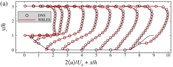
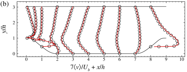
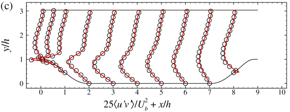
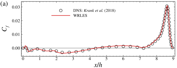
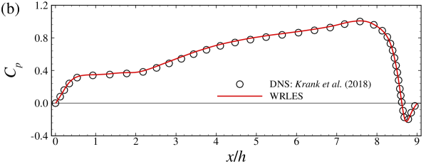
To validate the employed numerical method and case setup, we compare the profiles of the mean velocity, Reynolds shear stress, turbulence kinetic energy, and the skin friction and pressure coefficients computed in this work with the results from measurements Temmerman et al. (2003) and DNS by Krank et al. Krank et al. (2018) and demonstrate an overall good agreement as shown in Appendix A for validating the employed numerical method and case setup.
II.2 Data preparation
The WRLES data are further processed to prepare the data for training the data-driven wall model. In WMLES, the wall shear stress is often computed using the velocity at the first off-wall grid node. If the data-driven model is developed using the velocity at a specific location, it may only be applicable to grids of grid spacings. Moreover, if the wall model is developed using the data at a certain streamwise location, e.g. the location where the flow is attached or the location where flow separation occurs, it may only be valid for a certain flow condition. To avoid these two issues, we are devoted to develop a data-driven wall model applicable to different spatial resolutions and not limited to certain flow conditions using the data in the near-wall region of the periodic hills at all streamwise locations. Specifically in this work, the flow data in the near-wall region with wall-normal distance in the range of are employed, where denotes the wall-normal coordinate. The top boundary of the region at is determined considering that the flow field above is less correlated with the wall shear stress and is usually well-resolved by WMLES. It is noticed that the region with is defined as the inner layer for a turbulent channel flow, where is the half width of the channel. The bottom boundary at is defined to preclude the effects of viscous sublayer and with the consideration that no wall model is needed if the viscous scale is resolved.
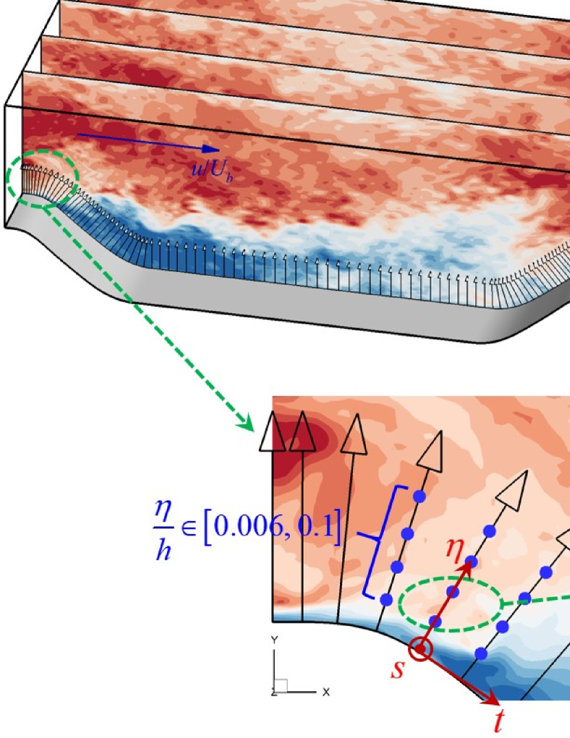
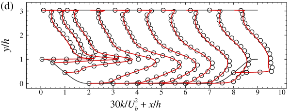
A step-by-step diagram for preparing the training data is shown in Figure 2. Saving the three-dimensional flow fields at every time step, which requires a significant amount of disk space, is not feasible. Instead, we save the WRLES data at four spanwise () slices located at , , and , respectively. To make the most of the WRLES data and meanwhile keep the cost for training the model at a reasonable level (in other words, avoid using the flowfields close in time, which can be very similar), 9 snapshots of the instantaneous flowfields are extracted on each slice for one flow-through time. And in total we obatain 450 snapshots for the whole flow-through times at each Reynolds number. For each snapshot, the flow field data at different wall-normal locations are further extracted at streamwise locations due to periodic boundary conditon to include different flow features along the lower wall of periodic hills. At each streamwise location of the lower wall, the flowfield data at 95 nodes, which are uniformly distributed in , are then extracted to form 95 pairs of input-output data along the wall-normal direction. Finally, the flowfield data along the wall-normal direction at different streamwise locations for all considered spanwise slices and snapshots form the complete training and testing datasets, which contain approximately input-output pairs. It is noticed that the grid nodes in the wall-normal () direction in general do not coincide with the curvilinear grid nodes employed for solving the flow. The linear interpolation approach based on triangulation is employed to obtain the flowfield data at the 95 points along the wall-normal coordinate.
Input features and output labels are critical for the success of data-driven models. The wall shear stress including the streamwise and spanwise stresses , , which are often applied as boundary conditions for outer flow simulations in WMLES, are employed as the output labels. To prepare the dataset for model training, the wall shear stresses are directly calculated using the WRLES data. As for the input features, the wall-normal distance , the three velocity components , and in the wall-tangential, -normal and spanwise directions and the pressure gradients , in the wall-tangential and -normal directions are employed. It has been shown by Duprat et al. Duprat et al. (2011) that using a near-wall scaling defined with the classic friction velocity and the streamwise pressure gradient can improve the performance of wall models for separated flows. To take into account such knowledge when constructing the neural networks for data-driven wall models, the wall-normal distance normalized using the near-wall scale and written in the logarithmic form, i.e. , where , , , , is employed as the input feature for training the data-driven wall model. Here the wall shear stress is computed as , which implicitly accounts for no-slip boundary conditions at the wall and approximates the wall shear stress resolved in WMLES. To further improve the generality of the trained model, the pressure gradients are multiplied by before taken as input features as suggested by Yang, Bose and Moin Yang et al. (2017b).
III Construction of data-driven wall models
III.1 Feedforward neural network
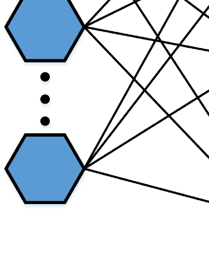
We use a multi-hidden-layer feedforward nueral network (FNN) to establish the relation between the near-wall flow and the wall shear stress on the surface of periodic hills. As shown in Figure 3, the employed FNN consists of an input layer, multi hidden layers and an output layer. Each layer has a number of neurons, which are computational units that propagate the weighted sums of the inputs to an activation function and calculate the output. The detailed procedures for calculating the output based on the input in the FNN is shown in Appendix B, which includes the linear matrix manipulation of the weight and bias coefficients and the nonlinear mapping using the activation function.
The activation function used in this paper is the rectified linear unit (ReLU) (Goodfellow et al., 2016),
| (4) |
The prepared input and output data are normalized using the Min-Max scaling,
| (5) |
The loss function is defined as
| (6) |
where is the number of training samples, is the weight coefficient, and is the regularization rate, which is set to 0.001. The first term in Eq. (6) denotes the mean square error (MSE) between the FNN output and the labeled output from the WRLES. The second term is an L2 regularization term included to avoid overfitting.
We use the error backpropagation (BP) scheme [56] implemented with TensorFlow [57] to train the FNN by optimizing the weight and bias coefficients to minimize the loss function. The key steps for FNN training are as follows:
(1) Provide training data to the input layer, propagate data signal forward layer by layer, and compute the result in the output layer. Details on this step can be found in Appendix B.
(2) Compute the loss function according to Eq. (6) using FNN output and the labeled output.
(3) Adjust the weight and bias coefficients using the gradient descent algorithm,
| (7) |
where denotes the weight and bias coefficients in the FNN, denotes the learning rate, which is dynamically adjusted using the Adam optimizer Kingma and Ba (2014).
(4) Repeat the above steps until the stop criterion is met.
III.2 Training of the data-driven wall model
In this section, three sets of cases, i.e. one with different number of input features, the other one with different number of neurons in each hidden layer, and the third one with different number of output labels, are carried out to evaluate the performance of different setups for training wall model using FNN and the flow data at and . The key requirement for a wall model is to accurately predict the wall shear stress. In conventional wall models, the wall shear stress is determined by an empirical relation (e.g. the power law or the logarithmic law) or simplified Navier-Stokes equations (e.g. the thin boundary layer equation) using the velocity at one off-wall grid node (usually the first or the second off-wall node). To compensate the lack of governing equations in data-driven wall models, flowfield data at more than one off-wall grid nodes are probably needed. In the first set of cases, we test the effects of input features obtained using different numbers of wall-normal points (five inputs per point) with the distance between two adjacent points . How well a data-driven model represents near-wall turbulence with flow separations and reattachments depends on the complexity of the employed neural network, i.e. the number of hidden layers and the number of neurons in each layer. In the second set of cases, we examine the effects of the number of neurons ranging from 3 to 100 on the training performance with fixed number of hidden layers and input features. Details on these two sets of cases can be found in Table 2.
| # of inputs (# per point # of points) | # of neurons (# of hidden layer) | |
|---|---|---|
| Case set 1 | (1, 2, 3, 4, 5, 6) | N20 (H6) |
| Case set 2 | N3, N5, N10, N20, N50, N100 (H6) |
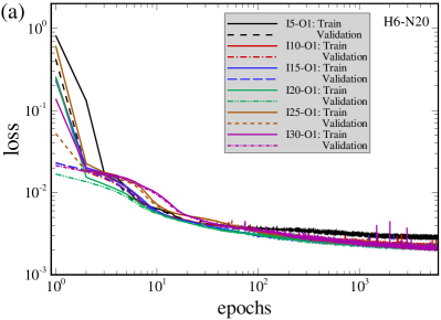
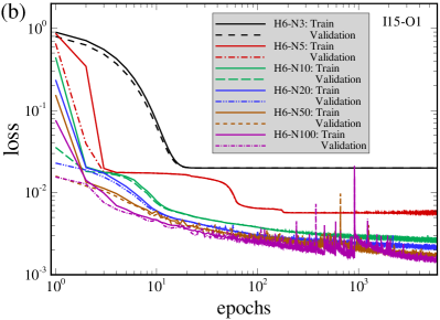
Figure 4 plots the variations of loss with the training epochs for both training and validation datasets for the two sets of cases. The number of training samples is , of which are used as the training dataset and the rest are used as validation dataset, and the batch size is . Intially, the loss is large because the weight coefficients are randomly set and the bias coefficients are set to zero. Then, the weight and bias coefficients are adjusted and the loss rapidly decreases during the first few epochs. After the initial stage, the loss tends to approch a steady small value after approximately 1000 training epochs.
In Figure 4(a), the loss in the FNN model I5-O1 (only using input features at one wall-normal point) is significantly worse than the other models, that the loss at 6000 epochs is about 1.5 times larger than others, while the values of loss from the models using input features at more than 1 points are similar with each other. This indicates that only using the input features at one point is not surfficient to accurately model the complex near-wall turbulence encountered in this periodic hill case, while adding just one point can significantly improve the training performance. To ensure the training performance without increasing the computational cost in the meantime, we choose 15 input features from 3 wall-normal points for case set 2 and other cases in this work. Figure 4(b) compares the loss of FNN models with different number of neurons. If no overfitting occurs, the more neurons are employed, the smaller the loss can be obtained. In this work we use 20 neurons for the proposed FNN wall model.
| FNN | Input | Output | HL size |
|---|---|---|---|
| FNN-1 | (, , , , ) 3 | H6-N20 | |
| FNN-2 | (, , , , , ) 3 | , |
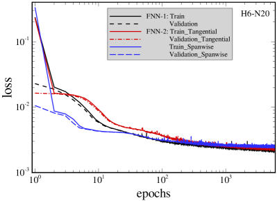
To consider the influence of output labels on the FNN training, the model ‘FNN-1’ with only one output label () and ‘FNN-2’ with two output labels (, ) are trained, validated and tested, respectively. The settings of the two FNN wall models are shown in Table 3. Figure 5 shows the variations of loss with training epochs for FNN-1 and FNN-2. It can be observed that including the spanwise wall shear stress as the output label has some effects on the model training process for epochs less than 100 but little influence on the final loss of tangential wall shear stress.
IV Evaluation of data-driven wall models
IV.1 Accuracy test
To evaluate the prediction accuracy and generalization capacity of the trained FNN wall model, we apply it to predict the wall shear stress for different snapshots and spanwise slices for both training datasets and testing datasets obtained from the cases with and .
We first evaluate the FNN wall models for predicting wall shear stresses using the training dataset. In Figure 6 we show the comparison of the instantaneous friction coefficient (which is defined as ) at an instant, the correlation coefficient between the instantaneous wall shear stress predicted by the FNN model and the WRLES, and the error of the instantaneous wall shear stress predicted by the FNN model relative to the WRLES predictions. Here, the correlation coefficient is defined as
| (8) |
where denotes the average over snapshots.
To further assess the prediction accuracy of FNN model on the fluctuations of wall shear stress over time, we define the instantaneous relative error as follows:
| (9) |
where denotes the peak value of averaged wall shear stress among all the streamwise locations. The relative error of the time-averaged wall shear stress, which will be shown in Figure 7(d), is defined as follows:
| (10) |
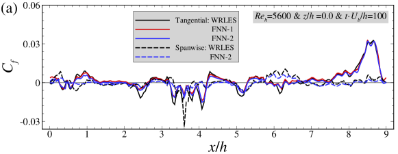
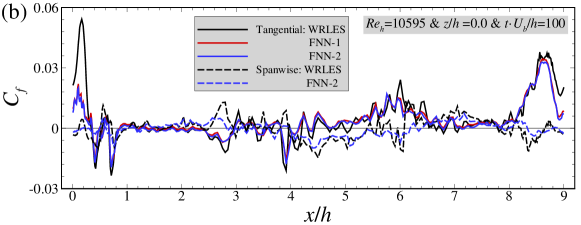
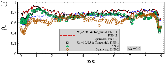
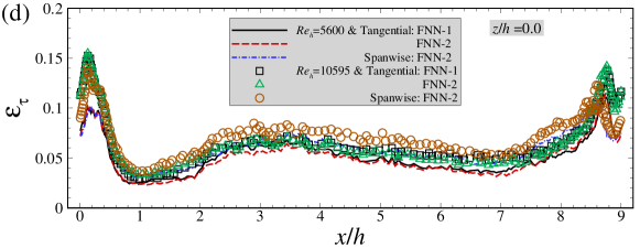
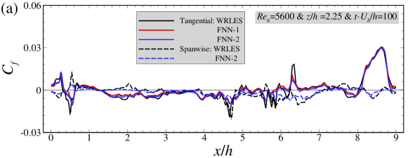
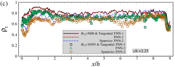
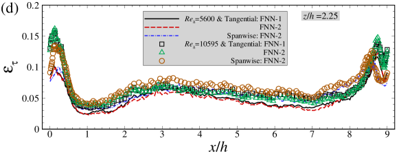
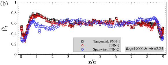
As seen in Figure 6(a)(b), the instantaneous skin friction coefficient predicted by the FNN model in general agrees with that from WRLES at most streamwise locations. Many sharp peaks are observed in streamwise variation of the instantaneous wall shear stress. The trained FNN wall model is observed being able to predict these abrupt variations at most streamwise locations, although the peak amplitude is underpredicted at some locations, e.g. at for this instant for the case.. It is also noticed that the wall tangential component of wall shear stress predicted by the FNN-1 and FNN-2 almost collapse with each other. Moreover, the spanwise component of the wall stress predicted by the FNN-2 model is also in good agreement with the WRLES predictions. In Figure 6(c)(d), it is observed that the correlation coefficients are larger than 0.7 and the instantaneous relative errors are smaller than 0.1 at almost all streamwise locations except near the crest of the hill at and (where the correlation coefficient is around 0.6, the instantaneous relative error is around 0.15), indicating that the large temporal fluctuations there are not well captured by the FNN model. It is noticed that correlation coefficient for the spanwise wall shear stress is similar with that of the tangential wall shear stress although the magnitude of the instantaneous spanwise wall shear stress is one order of magnitude smaller than the tangential component, which makes it difficult to train the corresponding FNN model for both components.
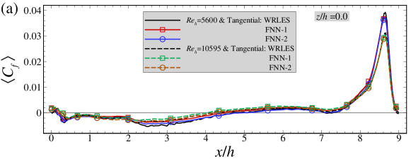
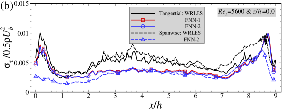
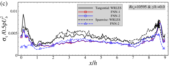
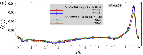
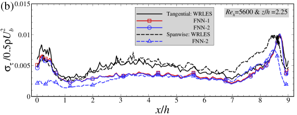
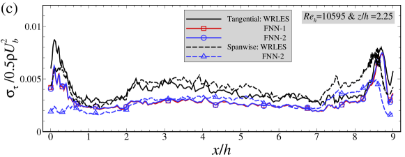
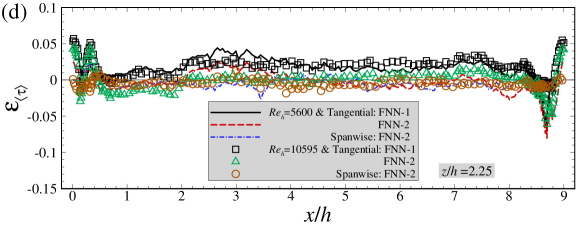
In Figure 7, we evaluate the capability the FNN model in predicting the mean wall shear stress and the standard deviation of wall shear stress. As seen in Figure 7(a), the mean skin friction coefficients at both and predicted by the FNN models (i.e. FNN-1 and FNN-2) are in perfect agreement with WRLES results at all streamwise locations. The mean spanwise wall shear stress component, on the other hand, is close to zero for both FNN-2 and WRLES predictions (not shown in the figure). In Figure 7(b)(c), we compare the normalized standard deviations of the fluctuations of wall shear stresses predicted by the FNN models with those from WRLES. It is observed that the FNN predictions are smaller than the WRLES predictions for both tangential and spanwise components. Interestingly, it is observed that the standard deviation of the spanwise shear stress is similar with the tangential component although its instantaneous value is one order of magnitude smaller than the tangential component. Figure 7(d) shows the error of time-averaged wall shear stress predicted by the FNN model relative to that from WRLES. It is seen that the absolute values of the errors are smaller than 0.05 at most streamwise locations, except at locations close to the crest of the hill.
Overall, we have shown that both FNN-1 and FNN-2 wall models can accurately predict the instantaneous and time-averaged wall shear stresses for the training dataset. Next, we will evaluate the performance of the FNN wall models using the testing dataset, which is obtained from a different slice (located at ) from the cases with and totally different from the training dataset.
In Figure 8, we first evaluate the capability of the FNN models in predicting the instantaneous wall shear stress using the testing dataset. As seen in Figure 8(a)(b), both tangential and spanwise instantaneous skin friction coefficients predicted by the FNN models are in an overall good agreement with the WRLES predictions except for some sharp peaks. Figure 8(c)(d) show the correlation coefficient and relative error between the FNN and LES predictions. As seen in the range of to , the correlation coeffcients are in general larger than 0.7 and the relative errors are smaller than 0.1 for both tangential and spanwise components. At locations close to the crest of the hill, lower coefficients and larger errors are observed especially close the separation point for the spanwise component.
In Figure 9, we compare the mean skin friction coefficients (averaged over snapshots), the standard deviations of the fluctuations and the time-averaged relative error of wall shear stresses predicted by different FNN wall models. As seen in Figure 9(a), good agreements between the FNN and WRLES predictions at and are obtained for the mean friction coefficients for both FNN models. For the standard deviations of the wall shear stresses, the predictions by the FNN models are significantly smaller than those from WRLES for both tangential and spanwise components. In Figure 9(d), the relative errors are smaller than 0.05 at most streamwise locations, which are close to the results in the training dataset.
IV.2 Application to different Reynolds numbers
To further evaluate the generalization capacity of the FNN wall model, we apply the trained FNN wall models to the testing dataset at in this section.
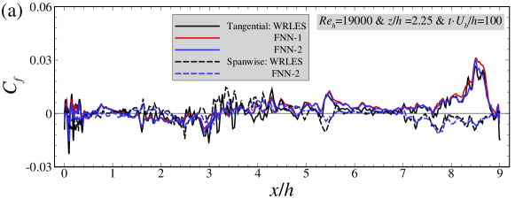
Figures 10 and 11 evaluate the predictive capability of the FNN models on the instantaneous and mean wall shear stresses, respectively. We first examine the predictons of the instantaneous skin friction coefficient. As shown in Figure 10(a), the FNN predictions are consistent with those from WRLES at most streamwise locations. The correlation coeffcients (Figure 10(b)) of instantaneous wall shear stresses between the FNN and LES predictions are also observed in general larger than 0.6 in the range of to , although they are somewhat smaller than those computed using the training dataset. The instantaneous relative errors are then examined in Figure 10(d). It is observed that the magnitude of the errors are slightly larger than those in training dataset, but still smaller than 0.1 at most streamwise locations.
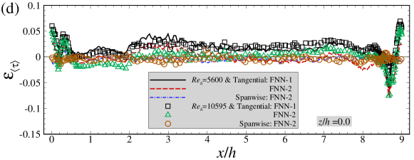
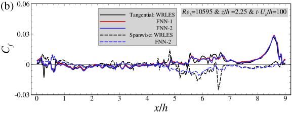
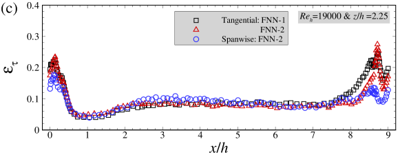
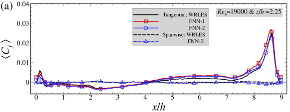
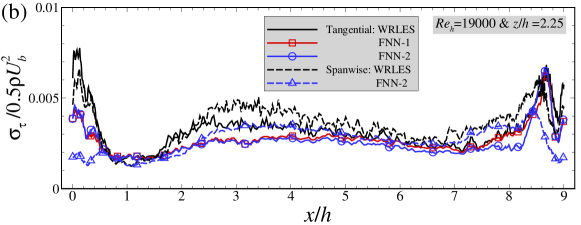
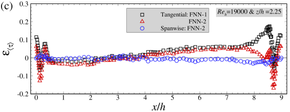
Here we examine the performance of the FNN models for predicting the mean skin friction coefficient. As seen in Figure 11(a), the mean skin friction coefficients at predicted by the FNN-2 model are in good agreement with WRLES results at all streamwise locations. Some discrepancies are observed between the FNN-1 predictions and the WRLES predictions highlighting the importance of having the spanwise wall shear stress as one of the output labels. As expected, the mean spanwise wall shear stress component is close to zero for both FNN model predictions and WRLES predictions. Similar with those observed in the cases with and , the normalized standard deviations of wall shear stress fluctuations predicted by the FNN models are smaller than those from WRLES, as shown in Figure 11(b). In Figure 11(d), the relative errors of the time-averaged wall shear stress are smaller than 0.1 at most streamwise locations, which are slightly larger than those computed using the training dataset. It is also noticed that the magnitude of the relative error for the predictions from the FNN-2 model is smaller than that from the FNN-1 model especially at locations around .
Although further improvement is still needed for the FNN wall model to accurately predict the standard deviations of wall shear stress fluctuations, the evaluations against the testing datasets at different Reynolds numbers demonstrate the excellent generalization capacity of the trained FNN wall models.
V Conclusion
As a first step towards developing a general wall model for complex turbulent flows, in this work we developed a data-driven wall model for LES of flow over periodic hills using the physics-informed feedforward neural networks and WRLES data.
Data preparation is critical for the success of training data-driven wall models. As the objective of this work is to develop a wall model that is applicable to different streamwise locations (of different flow regime, i.e. attached wall turbulence, flow separation and reattachment) of the periodic hill, the flow data near the surface of the hill at all streamwise locations are grouped together as the training data. The wall shear stresses are taken as the ouput labels. The input features include wall-normal distance, different components of velocity and pressure gradient at different wall-normal locations.
Effects of number of input features and number of neurons in the hidden layers on training performance were tested. It was found that using the flow data at more than two off-wall locations (in addition to the velocity at the boundary, which is implicitly taken into account) are adequate for training the data-driven wall model. Further increasing the number of input features does not improve the convergence rate when training the model. Employing more than 20 neurons in each hidden layer is found enough for this case. In the data-driven model developed in this work, flow data at three off-wall locations are employed as input features with 20 neurons for each hidden layer. Two different wall models, i.e. one using only the tangential wall shear stress as the output label (FNN-1), and the other one using both wall shear stress components as the output labels (FNN-2), are tested.
The prediction accuracy and generalization capacity of the trained FNN wall model were examined by comparing the predicted wall shear stresses with the WRLES data. The instantaneous wall shear stresses predicted by the FNN wall model show an overall good agreement with the WRLES data with some discrepancies observed at locations near the crest of the hill. For the mean wall shear stress, the predictions from the FNN wall models agree very well with WRLES data. However, the standard deviations of the fluctuations of the wall shear stress are underpredicted by the FNN wall model. Furthermore, it is noticed that the predictions from the two models, i.e. FNN-1 and FNN-2, are very similar with each other for the and cases, which are employed for training the model. For the case, for which the flow data are not employed for training the model, the FNN-2 model is observed performing better than the FNN-1 model. In summary, good performance and generalization capacity are observed for the developed FNN wall models. Implementation of the developed FNN wall model in WMLES and evaluation of its performance using a posteriori LES will be carried out in our future work.
Acknowledgements.
This work is partly supported by NSFC Basic Science Center Program for “Multiscale Problems in Nonlinear Mechanics” (No. 11988102) and National Natural Science Foundation of China (No. 12002345).Appendix A Details on the employed grid and validation of the present WRLES case
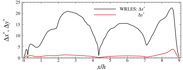
In this appendix, we show some details on the employed grid and validate the employed VFS-Wind code and the case setup for simulating turbulent flows over periodic hills at by comparing our WRLES results with the DNS results by Krank et al. Krank et al. (2018) ( grid points). Figure 12 shows the distribution of the grid spacings in wall units for and direction along the lower wall, where denotes the streamwise grid spacing in wall unit. The height of the first off-wall grid nodes in wall units, , is in the range of 0.056 to 3.95.
In Figure 13, we plot the vertical profiles of the time-averaged streamwise velocity and vertical velocity , primary Reynolds shear stress , turbulence kinetic energy . As seen, the WRLES results are in good agreement with the DNS results Krank et al. (2018) except for some minor differences observed in the Reynolds shear stress and the turbulence kinetic energy (with the relative error less than ). Figure 14 shows the comparison of the skin friction coefficient and the pressure coefficient . Again, the and from the present WRLES agree very well with the DNS predictions.
Appendix B Feedforward neural network
The detailed procedures for calculating the output based on the input in the FNN are described in this appendix.
The input layer is
| (11) |
where denotes the input feature, is the number of neurons in the input layer. The matrixes of weight and bias coefficient connecting the input layer and the hidden layer are
| (12) |
where denotes the weight coefficient connecting the neuron in the hidden layer and the neuron in the input layer, denotes the bias coefficient for the neuron in the hidden layer, is the number of neurons in the hidden layer. Initially, the weight coefficients are set to be random numbers from truncated normal distribution (0.0 mean and 0.1 standard deviation) and the bias coefficients are set to zero.
The output of the hidden layer is
| (13) |
where denotes the activation function to carry out the nonlinear mapping of the FNN, and the superscript “T” denotes the transpose of matrix. After the data transmission of multi hidden layers, the matrixes of weight and bias coefficient connecting the last hidden layer and the output layer are
| (14) |
where denotes the weight coefficient connecting the neuron in the output layer and the neuron in the hidden layer, denotes the bias coefficient for the neuron in the output layer and is the number of neurons in the output layer.
The output of the FNN is calculated by
| (15) |
References
- Moin and Mahesh (1998) P. Moin and K. Mahesh, “Direct numerical simulation: A tool in turbulence research,” Annu. Rev. Fluid Mech. 30, 539–578 (1998).
- Choi and Moin (2012) H. Choi and P. Moin, “Grid-point requirements for large eddy simulation: Chapman’s estimates revisited,” Phys. Fluids 24, 011702 (2012).
- He et al. (2017) G. W. He, G. D. Jin, and Y. Yang, “Space-time correlations and dynamic coupling in turbulent flows,” Annu. Rev. Fluid Mech. 49, 51–70 (2017).
- Piomelli and Balaras (2002) U. Piomelli and E. Balaras, “Wall-layer models for large-eddy simulations,” Annu. Rev. Fluid Mech. 34, 349–374 (2002).
- Cabot and Moin (2000) W. Cabot and P. Moin, “Approximate wall boundary conditions in the large-eddy simulation of high Reynolds number flow,” Flow Turbul. Combust. 63, 269–291 (2000).
- Davidson (2009) L. Davidson, “Large eddy simulations: How to evaluate resolution,” Int. J. Heat Fluid Flow 30, 1016–1025 (2009).
- Piomelli (2008) U. Piomelli, “Wall-layer models for large-eddy simulations,” Prog. Aerosp. Sci. 44, 437–446 (2008).
- Bose and Park (2018) S. T. Bose and G. I. Park, “Wall-modeled large-eddy simulation for complex turbulent flows,” Annu. Rev. Fluid Mech. 50, 535–561 (2018).
- Duraisamy et al. (2019) K. Duraisamy, G. Iaccarino, and H. Xiao, “Turbulence modeling in the age of data,” Annu. Rev. Fluid Mech. 51, 357–377 (2019).
- Brunton et al. (2020) S. L. Brunton, B. R. Noack, and P. Koumoutsakos, “Machine learning for fluid mechanics,” Annu. Rev. Fluid Mech. 52, 477–508 (2020).
- Pope (2000) S. B. Pope, Turbulent flows (Cambridge University Press, Cambridge, 2000).
- Wang and Moin (2002) M. Wang and P. Moin, “Dynamic wall modeling for large-eddy simulation of complex turbulent flows,” Phys. Fluids 14, 2043 (2002).
- Kawai and Larsson (2013) S. Kawai and J. Larsson, “Dynamic non-equilibrium wall-modeling for large eddy simulation at high Reynolds numbers,” Phys. Fluids 25, 015105 (2013).
- Park and Moin (2014) G. I. Park and P. Moin, “An improved dynamic non-equilibrium wall-model for large eddy simulation,” Phys. Fluids 26, 015108 (2014).
- Yang et al. (2015a) X. I. A. Yang, J. Sadique, R. Mittal, and Meneveau C., “Integral wall model for large eddy simulations of wall-bounded turbulent flows,” Phys. Fluids 27, 025112 (2015a).
- Chung and Pullin (2009) D. Chung and D. I. Pullin, “Large-eddy simulation and wall modelling of turbulent channel flow,” J. Fluid Mech. 631, 281–309 (2009).
- Cheng et al. (2015) W. Cheng, D. I. Pullin, and R. Samtaney, “Large-eddy simulation of separation and reattachment of a flat plate turbulent boundary layer,” J. Fluid Mech. 785, 78–108 (2015).
- Bose and Moin (2014) S. T. Bose and P. Moin, “A dynamic slip boundary condition for wall-modeled large-eddy simulation,” Phys. Fluids 26, 015104 (2014).
- Bae et al. (2018) H. J. Bae, A. Lozano-Durán, S. T. Bose, and P. Moin, “Turbulence intensities in large-eddy simulation of wall-bounded flows,” Phys. Rev. Fluids 3, 014610 (2018).
- Larsson et al. (2016) J. Larsson, S. Kawai, J. Bodart, and I. Bermejo-Moreno, “Large eddy simulation with modeled wall-stress: Recent progress and future directions,” Mechanical Engineering Reviews 3, 15–00418 (2016).
- Frere et al. (2018) A. Frere, K. Hillewaert, L. P. Chatelain, and G. Winckelmans, “High Reynolds number airfoil: From wall-resolved to wall-modeled LES,” Flow Turbul. Combust. 101, 457–476 (2018).
- Bae et al. (2019) H. J. Bae, A. Lozano-Duran, S. T. Bose, and P. Moin, “Dynamic slip wall model for large-eddy simulation,” J. Fluid Mech. 859, 400–432 (2019).
- Ling et al. (2016a) J. Ling, A. Kurzawski, and J. Templeton, “Reynolds averaged turbulence modelling using deep neural networks with embedded invariance,” J. Fluid Mech. 807, 155–166 (2016a).
- Zhou et al. (2019) Z. D. Zhou, G. W. He, S. Z. Wang, and G. D. Jin, “Subgrid-scale model for large-eddy simulation of isotropic turbulent flows using an artificial neural network,” Comput. Fluids 195, 104319 (2019).
- King et al. (2018) R. King, O. Hennigh, A. Mohan, and M. Chertkov, “From deep to physics-informed learning of turbulence: Diagnostics,” arXiv:1810.07785v2 (2018).
- Lee and You (2019) S. Lee and D. You, “Data-driven prediction of unsteady flow over a circular cylinder using deep learning,” J. Fluid Mech. 879, 217–254 (2019).
- Fukami et al. (2019) K. Fukami, K. Fukagata, and K. Taira, “Super-resolution reconstruction of turbulent flows with machine learning,” J. Fluid Mech. 870, 106–120 (2019).
- Liu et al. (2020) B. Liu, J. P. Tang, H. B. Huang, and X. Y. Lu, “Deep learning methods for super-resolution reconstruction of turbulent flows,” Phys. Fluids 32, 025105 (2020).
- Ling et al. (2016b) J. Ling, R. Jones, and J. Templeton, “Machine learning strategies for systems with invariance properties,” J. Comput. Phys. 318, 22–35 (2016b).
- Wang et al. (2017) J.-X. Wang, J.-L. Wu, and H. Xiao, “Physics-informed machine learning approach for reconstructing Reynolds stress modeling discrepancies based on DNS data,” Phys. Rev. Fluids 2, 034603 (2017).
- Wu et al. (2018) J.-L. Wu, H. Xiao, and E. Paterson, “Physics-informed machine learning approach for augmenting turbulence models: A comprehensive framework,” Phys. Rev. Fluids 3, 074602 (2018).
- Gamahara and Hattori (2017) M. Gamahara and Y. Hattori, “Searching for turbulence models by artificial neural network,” Phys. Rev. Fluids 2, 054604 (2017).
- Maulik et al. (2018) R. Maulik, O. San, A. Rasheed, and P. Vedula, “Data-driven deconvolution for large eddy simulations of Kraichnan turbulence,” Phys. Fluids 30, 125109 (2018).
- Vollant et al. (2017) A. Vollant, G. Balarac, and C. Corre, “Subgrid-scale scalar flux modelling based on optimal estimation theory and machine-learning procedures,” J. Turbul. 18, 854–878 (2017).
- Milano and Koumoutsakos (2002) M. Milano and P. Koumoutsakos, “Neural network modeling for near wall turbulent flow,” J. Comput. Phys. 182, 1–26 (2002).
- Yang et al. (2019) X. I. A. Yang, S. Zafar, J.-X. Wang, and H. Xiao, “Predictive large-eddy-simulation wall modeling via physics-informed neural networks,” Phys. Rev. Fluids 4, 034602 (2019).
- Huang et al. (2019) X. L. D. Huang, X. I. A. Yang, and R. F. Kunz, “Wall-modeled large-eddy simulations of spanwise rotating turbulent channels-Comparing a physics-based approach and a data-based approach,” Phys. Fluids 31, 125105 (2019).
- Fröhlich et al. (2005) J. Fröhlich, C. P. Mellen, W. Rodi, L. Temmerman, and M. A. Leschziner, “Highly resolved large-eddy simulation of separated flow in a channel with streamwise periodic constrictions,” J. Fluid Mech. 526, 19–66 (2005).
- Temmerman et al. (2003) L. Temmerman, M. A. Leschziner, C. P. Mellen, and J. Fröhlich, “Investigation of wall-function approximations and subgrid-scale models in large eddy simulation of separated flow in a channel with streamwise periodic constrictions,” Int. J. Heat Fluid Flow 24, 157–180 (2003).
- Manhart et al. (2008) M. Manhart, N. Peller, and C. Brun, “Near-wall scaling for turbulent boundary layers with adverse pressure gradient,” Theor. Comput. Fluid Dyn. 22, 243–260 (2008).
- Duprat et al. (2011) C. Duprat, G. Balarac, O. Métais, P. M. Congedo, and Brugière O., “A wall-layer model for large-eddy simulations of turbulent flows with/out pressure gradient,” Phys. Fluids 23, 015101 (2011).
- Breuer et al. (2009) M. Breuer, N. Peller, Ch. Rapp, and M. Manhart, “Flow over periodic hills - Numerical and experimental study in a wide range of Reynolds numbers,” Comput. Fluids 38, 433–457 (2009).
- Rapp and Manhart (2011) Ch. Rapp and M. Manhart, “Flow over periodic hills: an experimental study,” Exp. Fluids 51, 247–269 (2011).
- Krank et al. (2018) B. Krank, M. Kronbichler, and W. A. Wall, “Direct numerical simulation of flow over periodic hills up to =10,595,” Flow Turbul. Combust. 101(2), 521–551 (2018).
- Xiao et al. (2020) H. Xiao, J.-L. Wu, S. Laizet, and L. Duan, “Flows over periodic hills of parameterized geometries: A dataset for data-driven turbulence modeling from direct simulations,” Comput. Fluids 200, 104431 (2020).
- Yang et al. (2015b) X. L. Yang, F. Sotiropoulos, R. J. Conzemius, J. N. Wachtler, and M. B. Strong, “Large-eddy simulation of turbulent flow past wind turbines/farms: the Virtual Wind Simulator (VWiS),” Wind Energy 18(12), 2025–2045 (2015b).
- Yang and Sotiropoulos (2018) X. L. Yang and F. Sotiropoulos, “A new class of actuator surface models for wind turbines,” Wind Energy 21(5), 285–302 (2018).
- Kang and Sotiropoulos (2012) S. Kang and F. Sotiropoulos, “Numerical modeling of 3D turbulent free surface flow in natural waterways,” Adv. Water Resour. 40, 23–36 (2012).
- Kang et al. (2014) S. Kang, X. L. Yang, and F. Sotiropoulos, “On the onset of wake meandering for an axial flow turbine in a turbulent open channel flow,” J. Fluid Mech. 744, 376–403 (2014).
- Khosronejad and Sotiropoulos (2014) A. Khosronejad and F. Sotiropoulos, “Numerical simulation of sand waves in a turbulent open channel flow,” J. Fluid Mech. 753, 150–216 (2014).
- Yang et al. (2017a) X. L. Yang, A. Khosronejad, and F. Sotiropoulos, “Large-eddy simulation of a hydrokinetic turbine mounted on an erodible bed,” Renewable Energy 113, 1419–1433 (2017a).
- Yang and Sotiropoulos (2019a) X. L. Yang and F. Sotiropoulos, “On the dispersion of contaminants released far upwind of a cubical building for different turbulent inflows,” Build. Environ. 154, 324–335 (2019a).
- Yang and Sotiropoulos (2019b) X. L. Yang and F. Sotiropoulos, “Wake characteristics of a utility-scale wind turbine under coherent inflow structures and different operating conditions,” Phys. Rev. Fluids 4(2), 024604 (2019b).
- Foti et al. (2019) D. Foti, X. L. Yang, L. Shen, and F. Sotiropoulos, “Effect of wind turbine nacelle on turbine wake dynamics in large wind farms,” J. Fluid Mech. 869, 1–26 (2019).
- Khosronejad et al. (2020) A. Khosronejad, K. Flora, and S. Kang, “Effect of inlet turbulent boundary conditions on scour predictions of coupled LES and morphodynamics in a field-scale river: Bankfull flow conditions,” J. Hydraul. Eng. 146(4), 04020020 (2020).
- Germano et al. (1991) M. Germano, U. Piomelli, P. Moin, and W. H. Cabot, “A dynamic subgrid-scale eddy viscosity model,” Phys. Fluids A 3, 1760 (1991).
- Ge and Sotiropoulos (2007) L. Ge and F. Sotiropoulos, “A numerical method for solving the 3D unsteady incompressible Navier-Stokes equations in curvilinear domains with complex immersed boundaries,” J. Comput. Phys. 225(2), 1782–1809 (2007).
- Kang et al. (2011) S. Kang, A. Lightbody, C. Hill, and F. Sotiropoulos, “High-resolution numerical simulation of turbulence in natural waterways,” Adv. Water Resour. 34(1), 98–113 (2011).
- Yang et al. (2017b) X. Yang, S. Bose, and P. Moin, “A physics-based interpretation of the slip-wall LES model,” Center for Turbulence Research Annual Research Briefs (Stanford University, Stanford), 65–74 (2017b).
- Goodfellow et al. (2016) I. Goodfellow, Y. Bengio, and A. Courville, Deep Learning (MIT Press, Cambridge, MA, 2016).
- Kingma and Ba (2014) D. P. Kingma and J. Ba, “Adam: A method for stochastic optimization,” arXiv:1412.6980v9 (2014).