-meson twist-2 distribution amplitude within the QCD sum rules and investigation of
Abstract
In this paper, moments of -meson twist-2 light-cone distribution amplitudes were deeply researched by using QCD sum rules approach within background field theory. Up to 9th-order accuracy, we present at the initial scale , i.e. , , , , , respectively. An improved light-cone harmonic oscillator model for -meson twist-2 light-cone distribution amplitudes is adopted, where its parameters are fixed by using the least squares method based on the , and their goodness of fit reach to . Then, we calculate the transition form factors within the light-cone sum rules approach, and at largest recoil point, we obtain and . As a further application, the branching fractions of the semileptonic decays are given. Taking the decay into consideration, we obtain , , which are consistent with the BESIII collaboration and PDG data within errors. Finally, we present the angle observables of forward-backward asymmetries, -differential flat terms and lepton polarization asymmetry of the semileptonic decay .
pacs:
12.38.-t, 12.38.Bx, 14.40.AqI Introduction
In the past few decades, especially for the discovery of resonance state Ammar:1968zur , nature of scalar mesons below 1 GeV is a long-standing puzzle, which becomes one of hot topics in hadron physics. In the quark model scenario, the composition of has turned out to be mysterious. Its intriguing internal structure allows tests of various hypotheses, such as quark-antiquark Achasov:1987ts ; Cheng:2005nb , tetraquark states Jaffe:1976ig ; Alford:2000mm ; Humanic:2022hpq ; Brito:2004tv ; Klempt:2007cp ; Alexandrou:2017itd , two-meson molecule bound states Weinstein:1982gc ; Branz:2007xp ; Dai:2012kf ; Dai:2014lza ; Sekihara:2014qxa and hybrid states Ishida:1995 . However, until now there is no definite conclusion of which scenario is correct or have no general agreement on the inner structure of . Among the hadronic decay processes including state, semileptonic decay of charmed meson provides a simpler decay mechanism and final-state interactions, which can give an ideal platform for studying the meson’s properties.
From the experimental side, BESIII collaboration observed the charmless hadronic decay processes involving -meson, i.e. and with the significance up to and , respectively BESIII:2018sjg . Experimental facilities have reported the most precise results on the semileptonic decay of to pseudoscalar and vector mesons. From theory point of view, these channels are straightforward to study because the internal stucture/quark content of the meson is a typical quark-antiquark system. But the quark structure of the scalar meson below 1 GeV has varied explanations, cf. the review “Scalar mesons below 1 GeV” of Particle Data Group (PDG) ParticleDataGroup:2022pth . Wang et al. conclude the ratio provides a model independent way to distinguish the quark components of the light scalar meson, i.e. the four-quark and two-quark pictures Wang:2009azc . And this value has not confirmed exactly from experiments. Nowadays, the two-quark picture are researched by some theoretical group, such as covariant confined quark model (CCQM) Soni:2020sgn , light-cone sum rule (LCSR) Cheng:2017fkw ; Huang:2021owr , AdS/QCD Momeni:2022gqb , perturbative QCD (pQCD) Rui:2018mxc and Bethe-Salpeter equation Santowsky:2021ugd . So it is also meaningful to reconsider the two-quark scenario in detail and to compare the experimental observable, which is also the starting point of this paper.
The important physical quantity for semileptonic decays is the transition form factors (TFFs). As is known that the analogous semileptonic TFFs are also the essential ingredients for the indirect search of new physics beyond the Standard Model Aslam:2009cv . Therefore, an accurate TFFs is crucial for the semileptonic decay process. The LCSR approach is one of an effective method in dealing with heavy to light decays, which makes the operator production expansion (OPE) into the increasing twist light-cone distribution amplitudes (LCDAs), i.e twist-2, 3, 4 LCDAs. The LCSR is suitable in the large and middle recoil region. In this paper, we will adopt the LCSR to recalculate the TFFs and the experimental observable. One of the key quantities that characterize the TFFs is the twist-2 LCDA, which describes the dominant momentum fraction distribution for each part of a meson. In general, the -meson twist-2 LCDA can be expanded as a Gegenbauer polynomial series
| (1) |
where and . The zeroth-order Gegenbauer moment is equals to zero, and the even Gegenbauer coefficients are highly suppressed, which exactly equal to zero under the approximation that ( are masses of two constituent quarks), and the LCDA of the scalar meson is then dominated by the odd Gegenabuer moments. In contrast, the odd Gegenbauer moments vanish for and mesons. Thus, the behavior of tends to antisymmetric form under the exchange in isospin symmetry. Currently, the -meson twist-2 LCDA is mainly coming from QCDSR by Cheng et al. Cheng:2005nb , which gives the first two nonzero -moments 222The -moments can be related with Gegenbauer moments directly, which the formulae can be found in Ref. Cheng:2005nb . In our previous work Zhong:2022lmn , based on the pionic leading-twist DA, we analyzed in detail the influence of different numbers of -moments included in the fitting, and found that when the order of -moments is not more than ten, the change of the number of -moments has an obvious impact on the fitting result. When the order of -moment is more than ten, the change of the number of -moments has a very small impact on the fitting results. Thus, the higher-order -moments should be given in order to get more accuracy behavior and get more accuracy predictions for the processes involving -meson.
To achieve this target, the QCDSR under the framework of background field theory (BFT) is one of the effective way Novikov:1983gd ; Hubschmid:1982pa ; Govaerts:1983ka ; Govaerts:1984bk ; Ambjorn:1982bp ; Ambjorn:1982en ; Reinders:1984sr ; Elias:1987ac ; Huang:1986wm ; Huang:1989gv . In this approach, the quark and gluon fields are composed by background fields and quantum fluctuations around them. By decomposing quark and gluon fields into classical background fields describing nonperturbative effects and quantum fields describing perturbative effects, BFT can provide clear physical images for the separation of long-range and short-range dynamics of OPE. At present, the BFT has been applied to calculate the LCDAs of pseudoscalar and vector/axial vector mesons Fu:2016yzx ; Hu:2021zmy ; Hu:2021lkl ; Zhong:2014jla ; Fu:2018vap ; Zhong:2016kuv ; Huang:2004tp ; Zhong:2011rg . Therefore, we will study the scalar -meson twist-2 LCDA by using BFT. To get a more accurate behavior of , a research scheme is used which combine the LCHO model and nonperturbative QCD sum rule for -moments. Specifically, a new QCD sum rule formula will be used due to the zeroth-order -moments can not be normalized in the whole Borel parameters region. In this paper, we will calculate the first five-order nonzero -moments and determine the LCHO model parameters with the least squares method. This scheme is used in the pion case Zhong:2021epq , and subsequently for the kaon leading-twist DA Zhong:2022ecl and -meson longitudinal twist-2 DA Hu:2021lkl .
The remaining parts of this paper are organized as follows. In Sec. II, we calculate the -meson twist-2 LCDA moments and introduce the LCHO model. A new improved model is proposed and the model parameters shall be obtained by fitting moment with the least square method. Section III gives the numerical results and discussions, which include the transition form factor, decay width, decay branching ratio of semileptonic decays . Meanwhile, the forward-backward asymmetries, the differential flat terms and lepton polarization asymmetry of the semileptonic decay are also given. Section IV is for a brief summary.
II Theoretical framework
The -meson have three types of states, one is -meson with component, the other is -meson with component, and the third one is -meson with . Based on the basic procedure of QCD sum rules, one can adopt the following two-point correlator to derive the sum rules for -meson twist-2 LCDA moments , which can be read off,
| (2) | |||||
where and take odd numbers. The currents are taken as and , which are mainly come from definitions of the scalar -meson twist-2 LCDA and twist-3 LCDA , which can be written as Cheng:2005nb
| (3) | |||
| (4) |
From one side, one can apply the OPE for the correlator, e.g. Eq. (2) in deep Euclidean region . The calculation is carried out in the framework of BFT Huang:1989gv . Based on the basic assumptions and Feynman rules of BFT, the correlator can be expanded into three terms including the quark propagators and the vertex operators,
| (5) |
where “Tr” indicates trace for the -matrix and color matrix, and indicate the light-quark propagator from to 0 and from 0 to . The are the vertex operators from current . The expressions up to dimension-six of the quark propagator, the vertex operator, and the vacuum matrix elements such as and have been derived in our previous works Zhong:2011rg ; Zhong:2014jla ; Zhong:2021epq ; Hu:2021zmy . By substituting those corresponding formula into Eq. (5), the OPE of correlator (2), , can be obtained. Meanwhlie, we take stand for the light , -quark. On the other hand, one can insert a complete set of -meson intermediated hadronic states with the same quantum number into the correlator and obtain the hadronic expression
| (6) |
with is the light quark mass, where the slight difference between mass of -quark and -quark is ignored in this paper. Meanwhile, the stands for the continuum threshold. Here the definitions of moments for -meson twist-2, 3 LCDAs are used, which have the following formula
| (7) | |||
| (8) |
where and stand for -meson mass and its decay constant, respectively. By considering the dispersion relation and performing Borel transformation, we can get the sum rule for ,
| (9) |
with . For a more thorough considering the sum rule for , it might be convenient to calculate . To achieve this target, one can use the correlator for the -meson twist-3 LCDA 0th moment. Followed by the basic procedure of the QCDSR, the expression of the 0th moment of scalar meson -meson twist-3 LCDA can be obtained,
| (10) |
Here, the light quark is taken as and corresponding vacuum condensates are given in the next Section. Since higher-order and higher-dimensional corrections are difficult to calculate completely, the moments of the sum rule (9) cannot be normalized in the intire Borel parameter region. To get a more accurate moments for sum rule, we can use the following expression
| (11) |
This method can eliminate the systematic errors caused by many factors. The discussion for the pion and kaon cases can be found in our previous work Zhong:2021epq ; Zhong:2022ecl .
Furthermore, -meson twist-2 DA describes the momentum fraction distribution of partons in -meson for the lowest Fock state. Due to the is the universal nonperturbative physical quantity, it should be researched by the nonperturbative QCD approach. Normally, one can study the based on the combination of nonperturbative QCD and phenomenological model. Meanwhile, conformal expansion of LCDAs Gegenbauer polynomials makes the higher-order Gegenbauer moments unreliable. To improve this situation, the LCHO is adopted to determine -meson twist-2 LCDA. Referring to the LCHO model of the pion leading-twist WF raised in Refs. Wu:2010zc ; Wu:2011gf , one can start with the Brodsky-Huang-Lepage (BHL) prescription, which assuming there is a connection between the equal-times wave function in the rest frame and the light-cone wave function BHL . it can be expressed as:
| (12) |
where is transverse momentum. Furthermore, and are the helicities of the two constituent quark. stands for the spin-space WF that comes from the Wigner-Melosh rotation. The different forms of are shown in Table 1, which can also been seen in Refs. Huang:1994dy ; Cao:1997hw ; Huang:2004su ; Wu:2005kq . The spin-space WF, e.g. . Then, by combing the spatial WF , the -meson WF will be obtained. Here, the , stand for the normalization constant and light quark mass. The final -meson twist-2 LCDA can be obtained by using the relationship between the twist-2 LCDA and WF of -meson, e.g. integrated over the squared transverse momentum, which can be expressed as
| (13) |
where is the error function, and . Based on the experience of other mesons Huang:2013gra ; Huang:2013yya ; Wu:2012kw ; Zhong:2015nxa ; Zhang:2021wnv ; Hu:2021lkl ; Zhong:2018exo ; Zhong:2022ecl ; Zhong:2021epq , we take the wavefunction parameter . Whether the value of is accurate can be judged by goodness of fit . The free parameters and can be obtained by fitting the moments with the least squares method directly.
In deriving the complete expression for TFFs, one can take the following correlator
| (14) |
with , . Followed by the standard LCSR approach, one can make the OPE near the light-cone in the space-like region, and insert a complete set of -meson states in the physical region. After performing the Borel transformation, we can get the TFFs up to twist-3 accuracy, which can be read off
| (15) | |||
| (16) |
Here the abbreviation is used. The lower limits of the integration is . Here, and are the mass and decay constant of -meson, is the -quark mass, , stands for the continuum threshold. and , are twist-2 and twist-3 LCDAs, respectively. The twist-3 LCDA can be found in Refs. Han:2013zg ; Lu:2006fr . Here, we have a notation that the analytical expressions for the sum rules of the TFFs, i.e. Eqs. (15) and (16) are equivalent with the tree-level LCSR for the exclusive heavy-to-light TFFs () have been previously constructed in Ref. Wang:2008da , without the surface term coming from the twist-3 LCDA contributions. In this paper, the TFFs analytical expressions are derived based on the pion cases Duplancic:2008ix , where the power of denominator is reduced by taking the derivative of the final state light-cone distribution amplitude.
Then, the explicit expression for the full differential decay width have the following form
| (17) | |||||
with the angular coefficient functions , and are Becirevic:2016hea
| (18) |
Here with and stand for CKM matrix element and fermi coupling constant. and stand for the leptonic mass and helicity angle. In the massless lepton limit, the angular functions , . In addition, with . The in the expression can be expressed as Fu:2013wqa . After integrating over the helicity angle , we can get the expression -dependence differential decay width Cheng:2017fkw ; Huang:2021owr
Furthermore, the TFFs are also the basic component of indirect search for new physics Beyond the Standard Model (BSM) phenomenologically. So the angular observables which are sensitive to BSM, i.e. the normalized forward-backward asymmetries, the -differential flat terms and lepton polarization asymmetry , , of the semileptonic decay , respectively. The relationships between these observables and TFFs are as follows Cui:2022zwm :
| (20) |
III Numerical analysis
To do the numerical analysis, we adopt meson’s mass , and . Besides, the current quark-mass are and at scale . The -meson decay constant is . The values of the non-perturbative vacuum condensates appearing in the BFTSR are given below as Narison:2014ska ; Colangelo:2000dp ; Zhong:2021epq ,
| (21) |
The values of the double-quark condensate , quark-gluon mixed condensate are at . Otherwise, these parameters can be calculated to any scale according to the evolution equation.
In the context of BFTSR, there are two important parameters the continuous threshold and the Borel parameter , respectively. We generally take the scale . Under the 3-loop approximate solution, the for the number of quark flavors , with which the , , and are used. Furthermore, the gluon or quark vacuum condensates and non-perturbative matrix element at initial scale can be running to other scales thought out the renormalization group equations RGE) Yang:1993bp ; Hwang:1994vp , which can be written as a general formula:
| (22) |
with which the function are , and for the , and , respectively. The coefficient and is the number of active quark flavors. According to the basic assumption of BFTSR, it is worth noting that is the coupling constant between background fields in the above vacuum condensates, which is different from the coupling constant in pQCD and should be absorbed into the vacuum condensates as part of these non-perturbative parameters. The RGE of the Gegenbauer moments of the -meson twist-2 LCDA is Cheng:2005nb :
| (23) |
with . The and represent the initial scale and the running scale, the one-loop anomalous dimensions is , with . According to the RGE of the Gegenbauer moments, one can get the moments for the arbitrary scale .
| Con. | |||
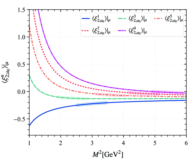
Furthermore, the continuum threshold parameter for the sum rule can be determined by normalization for , which leads to . Then, the Borel window for the each order of -meson LCDA moments can be determined by limiting the continuum states and the dimension-six condensates contributions. Then, the moments with within uncertainties coming from Borel parameters are listed in Table 2. Based on the BFTSR, the dimension-six condensates contributions for are less than for all the th-order. To get the suitable Borel window, the continuum contributions for are restrict to for respectively. Since the dimension-six condensates contributions are very small, we determine the upper limit of the Borel parameter through the continuum contributions. Then the lower limit of the Borel parameter can be determined by the method of the upper limits, so as to obtain the appropriate Borel window. At the same time, the values of the moments are stable in the appropriate Borel window. To have a deeper insight into the relationship of the LCDA moments versus Borel parameter , the first five moments’s curves are shown in Fig. 1, which can be seen that
-
•
In the region of Borel window, the curves for changed dramatically. With the increase of Borel window , the change trend of moments , , , , tends to be gentle.
-
•
With increases, the absolute value of the moments tend to be smaller.
Taking all the input uncertainties into consideration, we can get the moments with under two types of factorization scale and ,
| (24) |
Our results for the first two order are slightly smaller than the Cheng’s predictions, e.g. and by using the QCDSR approach from Ref. Cheng:2005nb , which is more likely to be antisymmetric behavior. The little difference may be related to the different methods in determining the continuum threshold . Meanwhile, the higher order such as are given for the first time. The new formulae Eq. (11) can reduce the systematic error of sum rules of the -moments, and it enables us to calculate higher-order moments to provide more complete information of DA.
| 200 MeV | |||
| 250 MeV | |||
| 300 MeV | |||
| 350 MeV |
Secondly, the free parameters and for the LCHO model can be fixed by adopting the method of least squares to fit calculated in the framework of the BFTSR shown in Eq. (24). The goodness of fit can be judged by the probability () 333For more details, one can see our previous work for pion Zhong:2021epq .. By fitting the moments at the scale , the optimal model parameters are obtained as follows,
| (25) |
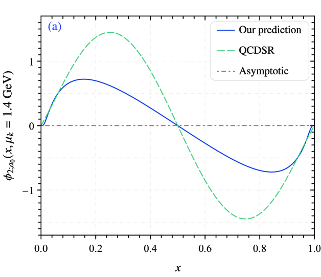
The above parameters are derived from . From these parameters, we obtain the scalar -meson twist-2 LCDA , which is shown in the left panel of Fig. 2. In the meantime, we also present the results of QCDSR Cheng:2005nb prediction as a comparison. From the perspective of variation trend, our prediction results are relatively consistent with the those of QCDSR, and twist-2 LCDA are both antisymmetric. However, there are also some differences between the two, which may be due to differences in calculation methods. The former uses the Gegenbauer moments polynomials expansion, while we take the LCHO model to construct LCDA .
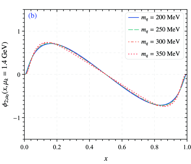
For further study, we also analyze the relationship between the goodness-fit of the -meson twist-2 LCDA and the quark mass listed in Table 3. It is obvious that as the quark mass increases, the goodness of fit also increases. The goodness of fit also indicates that is reasonable. Considering the effect of quark mass on the -meson twist-2 LCDA , the behavior of LCHO model for different quark masses is shown in the right panel of Fig. 2. As can be seen from the figure, the peak value of the LCHO model curves increases with the increase of mass . In addition to this, the relationship between goodness of fit and parameters and is also shown in Fig. 3. From the table we can see that the can reach to , which shows the fitting is good.
. This work CCQM Soni:2020sgn LCSR 2021 Huang:2021owr LCSR 2017 Cheng:2017fkw AdS/QCD Momeni:2022gqb -
The TFFs is an important parameter in the calculation of the semileptonic decay . To obtain the numerical results of TFFs, we take , ParticleDataGroup:2022pth , Cheng:2005nb . For the continuum threshold , it is generally taken near the mass square of the first excited state of -meson, that is, near the mass square of -meson. Based on the prediction of the sum rule of heavy quark effective theory (HQET) Huang:1998sa , we take the continuum threshold parameter . The adopted threshold parameter is consistent with the LCSR analysis for the heavy-to-heavy form factors with the bottom-meson distribution amplitudes as discussed in Ref. Li:2012gr ; Wang:2017jow .
According to LCSR, in the suitable Borel window, we predict the end values of the semileptonic decay TFFs shown in Table 4. As a comparison, the results predicted from various approaches, CCQM Soni:2020sgn , LCSR 2017 Cheng:2017fkw , LCSR 2021 Huang:2021owr and AdS/QCD Momeni:2022gqb also are presented in Table 4. It is not difficult to see from the Table 4 that our predicted results are significantly different from those obtained by other predictions. The reason lies in the twist-2 LCDA is different, which the LCHO model is used here.
| Central value | Upper limits | Lower limits | |
| 0.18‰ | 0.17‰ | 0.18‰ | |
| Central value | Upper limits | Lower limits | |
| 0.26‰ | 0.30‰ | 0.23‰ |
| This work | ||||
| CCQM Soni:2020sgn | ||||
| LCSR 2017 Cheng:2017fkw | - | - | ||
| LCSR 2021 Huang:2021owr | ||||
| AdS/QCD Momeni:2022gqb | - | - | - |
| This work | ||
| BESIII BESIII:2018sjg | ||
| LCSR 2021 Huang:2021owr | ||
| PDG ParticleDataGroup:2022pth |
In the physical sense, the LCSR method is suitable for in low and intermediate region. The physical region for TFFs is . In order to obtain reasonable LCSR results, we can extend them to the entire physical -region . Therefore, we can fit the complete analysis results with simplified series expansion (SSE), which is a rapidly convergent series on the -expansion Fu:2018yin ; Bharucha:2015bzk ; Bourrely:2008za .
| (26) |
where stands for TFFs, the fit coefficients,and
| (27) |
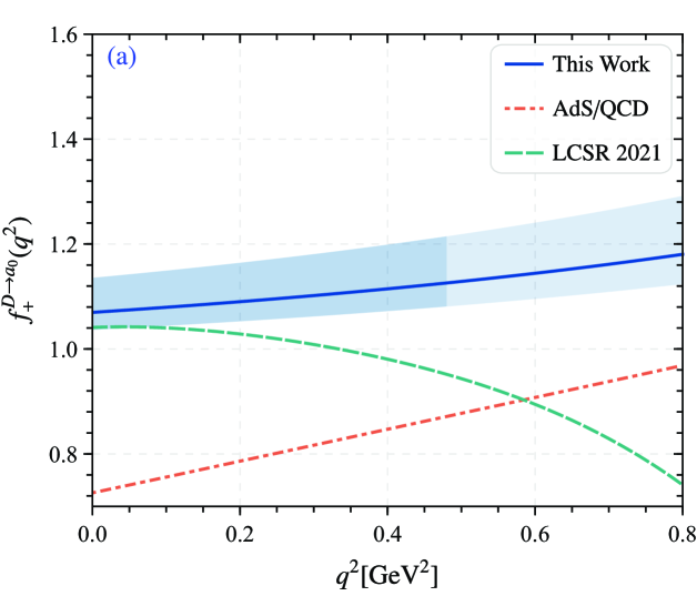
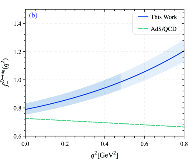
with , . is a simple pole corresponding to the first resonance in the spectrum. Meanwhile, there have another alternation version of the -series parametrization for the heavy-to-light TFFs from Wang and Shen Wang:2015vgv , which can also achieve this purpose. The fitting parameters for the TFFs within uncertainties are given in Table 5. Meanwhile, the goodness of fit with for each TFFs are also presented. After extrapolating TFFs to the whole region, the curves are shown in the Fig. 4. We also give the curves obtained by LCSR 2021 Huang:2021owr and AdS/QCD Momeni:2022gqb for comparison. The results show our prediction is a certain discrepancy between the results in Ref. Huang:2021owr . There are also some deviations from results predicted by AdS/QCD, but the curve trend is relatively consistent. In most cases, The shows an upward trend with the increase of . Our prediction is quite reasonable. The is also exhibit upward tendency and it turns out that there are some differences.
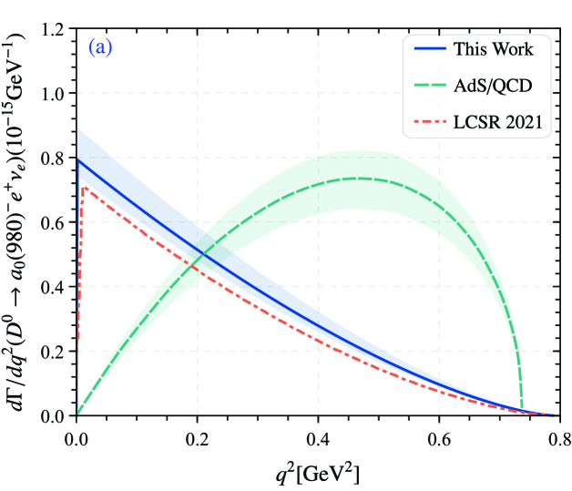
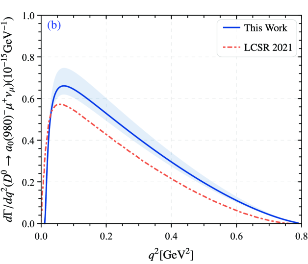
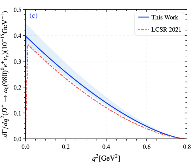
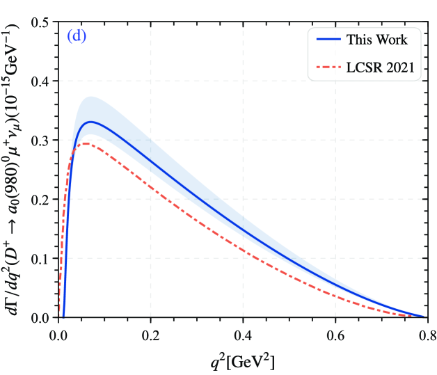
As other important parameters for , the CKM matrix element from the PDG ParticleDataGroup:2022pth , the fermi coupling constant . By taking the derived TFFs and the related parameters into the differential decay widths Eq. (II), one can get the differential decay widths of with presented in Fig. 5. For comparison, we also present the results of LCSR 2021 Huang:2021owr predictions in Fig. 5. The figure shows that our prediction is consistent with the result of LCSR 2021 within a certain error range. In Fig. 5(a), discrepancy between our prediction and the result of AdS/QCD, which may be caused by the different TFFs. Obviously, the predicted results converge to zero in the small recoil region . The shaded part in the figure is the error of the width, which mainly comes from the uncertainty of all parameters.
Furthermore, by taking the lifetimes of and meson and from PDG, we can obtain the branching ratio of semileptonic decay channels () and in Table LABEL:branching_ratios. What’s more, the predictions from theoretical groups such as CCQM Soni:2020sgn , LCSR Cheng:2017fkw ; Huang:2021owr , AdS/QCD Momeni:2022gqb are shown in Table LABEL:branching_ratios. It is obvious that our results are relatively consistent with those of CCQM and LCSR 2021 within the error. However, the significant difference between our predictions and LCSR 2017, AdS/QCD may be caused by the difference of the TFFs and -meson twist-2 LCDA.
. Observables Results
Additionally, we also calculate the absolute branching ratio of decays by using the relationship
| (28) |
Here the can be used Cheng:2005nb . Combing with the been calculated in this paper, we can get the results for and , which are listed in Table LABEL:ratios. For comparison, the results of the BESIII BESIII:2018sjg collaboration, theory groups LCSR 2021 Huang:2021owr and PDG ParticleDataGroup:2022pth predictions are also given. The results show that our predicted absolute branching ratio are in good agreement with those predicted of BESIII, LCSR 2021 and PDG within the error range. It is clear that our prediction is more accurate than the LCSR 2021 prediction, with an improvement of about . It shows that the result of our prediction is reasonable.
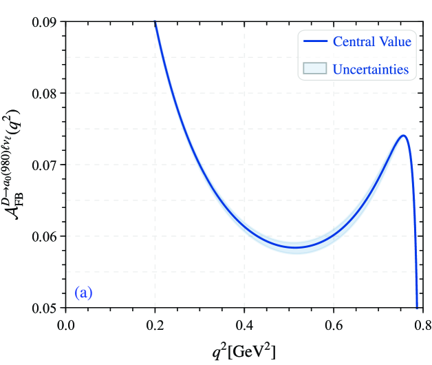
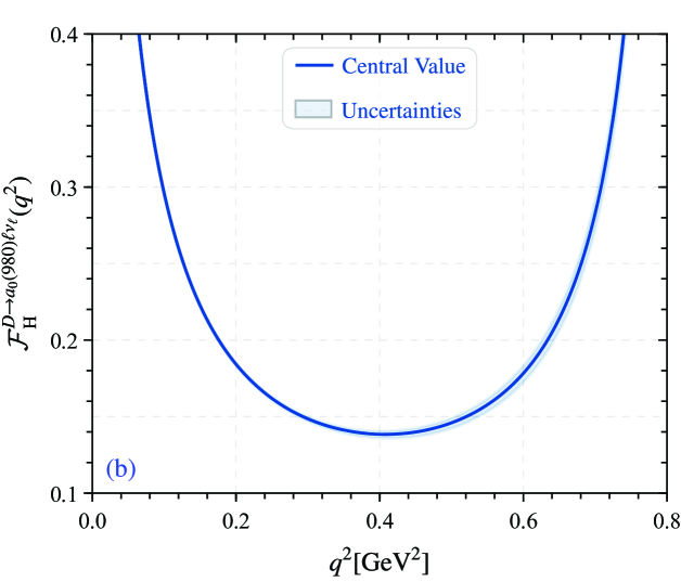
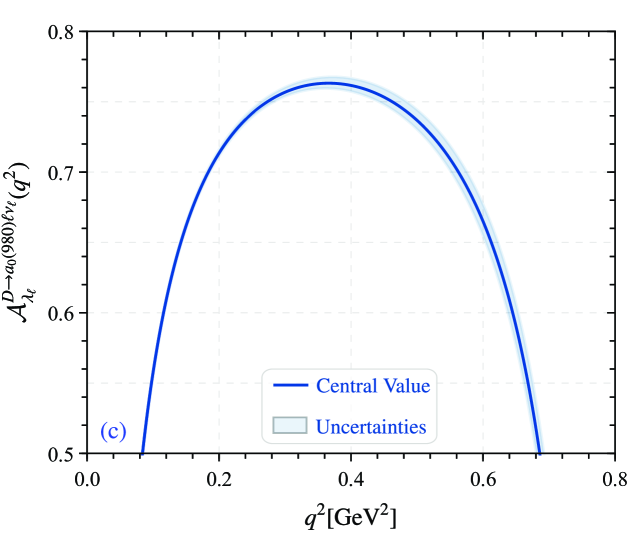
Finally, the three differential distribution of angle observables for forward-backward asymmetries, the -differential flat terms and lepton polarization asymmetry of the semileptonic decay , i.e. , and are shown in Fig. 6. The forward-backward asymmetries curves, i.e. Fig. 6(a) are different with pion and kaon cases Cui:2022zwm , while the -differential flat terms and lepton polarization asymmetry have the same tendency overall with pion and kaon cases, but have slight differences. Meanwhile, the uncertainties for the three angle observables are small. Finally, we present the integral results for the three observables in Table 8.
IV Summary
In this paper, we have calculated the moments of -meson twist-2 LCDA by adopting the QCDSR approach within the background field theory. The continuum threshold parameter is determined from the normalization for the -meson twist-3 LCDA 0th-order moments. After seeking the suitable Borel windows, we present the first five order moments, i.e. with under two different factorization scales and . Then, we study -meson twist-2 LCDA based on the LCHO model for improving the accuracy of the calculation. The least square method is used to fit the moments and to determine the model parameters. The goodness of fit can be up to . Then, the curves of -meson twist-2 LCDA comparing with other theoretical groups and with different constituent quark masses are presented.
The TFFs are calculated within the LCSR approach. The TFFs at large recoil region are listed in Table 4. After extrapolating the TFFs to the whole region, the curves are shown in Fig. 4. A comparison of TFFs with other LCSR and AdS/QCD predictions are also given. Using the resultant TFFs, we further studied the semileptonic decays with . Their differential decay widths are presented in Fig. 5, and their branching fractions are given in Table LABEL:branching_ratios. The ratio of partial branching fractions is given
| (29) |
which agree with the CCQM prediction Soni:2020sgn and the LCSR predictions Cheng:2017fkw ; Huang:2021owr within errors.
After considering the decay , we have calculated the branching fractions for the decay processes , and . The results of our predictions are consistent with the BESIII data and PDG average value within errors, which indicate the two-quark picture of is also reasonable in comparing with four-quark picture. Along with other results of branching fraction for scalar meson discovered experimentally, we will have a reliable input for understanding the nature of the light scalar mesons.
Finally, we also predicted the forward-backward asymmetries, the differential flat terms and lepton polarization asymmetry of the semileptonic decay . The overall behavior of , and as a function of is shown in Fig. 6, and the numerical results of the integration are listed in Table 8, which can provides phenomenology value for exploring other new physics.
Acknowledgements.
We are grateful for the referee’s valuable comments and suggestions. This work was supported in part by the National Natural Science Foundation of China under Grant No.12265010, No.12265009, No.12175025 and No.12147102, the Project of Guizhou Provincial Department of Science and Technology under Grant No.ZK[2021]024 and No.ZK[2023]142, the Project of Guizhou Provincial Department of Education under Grant No.KY[2021]030, and by the Chongqing Graduate Research and Innovation Foundation under Grant No. ydstd1912.References
- (1) R. Ammar, R. Davis, W. Kropac, J. Mott, D. Slate, B. Werner, M. Derrick, T. Fields and F. Schweingruber, Boson resonance of mass 980 MeV decaying into , Phys. Rev. Lett. 21, 1832-1835 (1968).
- (2) N. N. Achasov and V. N. Ivanchenko, On a Search for Four Quark States in Radiative Decays of phi Meson, Nucl. Phys. B 315 (1989), 465-476.
- (3) H. Y. Cheng, C. K. Chua and K. C. Yang, Charmless hadronic decays involving scalar mesons: Implications to the nature of light scalar mesons, Phys. Rev. D 73,014017 (2006). [hep-ph/0508104]
- (4) R. L. Jaffe, Multi-quark hadrons. 1. The phenomenology of mesons, Phys. Rev. D 15, 267 (1977).
- (5) M. G. Alford and R. L. Jaffe, Insight into the scalar mesons from a lattice calculation, Nucl. Phys. B 578, 367-382 (2000). [hep-lat/0001023]
- (6) T. Humanic [ALICE Collaboration], Studying the (980) tetraquark candidate using interactions in the LHC ALICE collaboration, Rev. Mex. Fis. Suppl.3, 0308039(2022) .
- (7) T. V. Brito, F. S. Navarra, M. Nielsen and M. E. Bracco, QCD sum rule approach for the light scalar mesons as four-quark states, Phys. Lett. B 608, 69-76 (2005). [hep-ph/0411233]
- (8) E. Klempt and A. Zaitsev, Glueballs, hybrids, multiquarks. Experimental facts versus QCD inspired concepts, Phys. Rept. 454 1-202 (2007). [arXiv:0708.4016]
- (9) C. Alexandrou, J. Berlin, M. Dalla Brida, J. Finkenrath, T. Leontiou and M. Wagner, Lattice QCD investigation of the structure of the meson, Phys. Rev. D 97, 034506 (2018). [arXiv:1711.09815]
- (10) J. D. Weinstein and N. Isgur, Do Multi-Quark Hadrons Exist?, Phys. Rev. Lett. 48, 659 (1982).
- (11) T. Branz, T. Gutsche and V. E. Lyubovitskij, -meson as a molecule in a phenomenological Lagrangian approach, Eur. Phys. J. A 37, 303 (2008). [arXiv:0712.0354]
- (12) L. Y. Dai, X. G. Wang and H. Q. Zheng, Pole Analysis of Unitarized One Loop PT Amplitudes - A Triple Channel Study, Commun. Theor. Phys. 58, 410-414 (2012). [arXiv:1206.5481]
- (13) L. Y. Dai and M. R. Pennington, Two photon couplings of the lightest isoscalars from BELLE data, Phys. Lett. B 736, 11-15 (2014). [arXiv:1403.7514]
- (14) T. Sekihara and S. Kumano, Constraint on compositeness of the and resonances from their mixing intensity, Phys. Rev. D 92, 034010 (2015). [arXiv:1409.2213]
- (15) S. Ishida et al. in Proceeding of the 6th International conference on Hadron Spectroscopy, Manchester, UK, 1995.
- (16) M. Ablikim et al. [BESIII Collaboration], Observation of the semileptonic decay and evidence for , Phys. Rev. Lett.121, 081802 (2018). [arxiv:1803.02166]
- (17) R. L. Workman et al. [Particle Data Group], Review of Particle Physics, PTEP 2022, 083C01 (2022).
- (18) W. Wang and C. D. Lu, Distinguishing two kinds of scalar mesons from heavy meson decays, Phys. Rev. D 82, 034016 (2010). [arXiv:0910.0613]
- (19) N. R. Soni, A. N. Gadaria, J. J. Patel and J. N. Pandya, Semileptonic decays of charmed mesons to light scalar mesons, Phys. Rev. D 102, 016013 (2020). [arXiv:2001.10195]
- (20) X. D. Cheng, H. B. Li, B. Wei, Y. G. Xu and M. Z. Yang, Study of decay in the light-cone sum rules approach, Phys. Rev. D 96, 033002 (2017). [arXiv:1706.01019]
- (21) Q. Huang, Y. J. Sun, D. Gao, G. H. Zhao, B. Wang and W. Hong, Study of form factors and branching ratios for with light-cone sum rules, [arXiv:2102.12241]
- (22) S. Momeni and M. Saghebfar, Semileptonic -meson decays to the vector, axial vector and scalar mesons in Hard-Wall AdS/QCD correspondence, Eur. Phys. J. C 82, 473 (2022).
- (23) Z. Rui, Y. Q. Li and J. Zhang, Isovector scalar and resonances in the decays, Phys. Rev. D 99, 093007 (2019). [arXiv:1811.12738]
- (24) N. Santowsky and C. S. Fischer, Light scalars: Four-quark versus two-quark states in the complex energy plane from Bethe-Salpeter equations, Phys. Rev. D 105, 034025 (2022). [arXiv:2109.00755]
- (25) M. J. Aslam, C. D. Lu and Y. M. Wang, decays in supersymmetric theories, Phys. Rev. D 79, 074007 (2009). [arXiv:0902.0432]
- (26) T. Zhong, Z. H. Zhu and H. B. Fu, Constraint of -moments calculated with QCD sum rules on the pion distribution amplitude models, arXiv:2209.02493.
- (27) V. A. Novikov, M. A. Shifman, A. I. Vainshtein and V. I. Zakharov, Calculations in external fields in quantum chromodynamics. Technical review, Fortsch. Phys. 32, 585 (1984).
- (28) W. Hubschmid and S. Mallik, Operator expansion at short distance in QCD, Nucl. Phys. B 207, 29-42 (1982).
- (29) J. Govaerts, F. de Viron, D. Gusbin and J. Weyers, Exotic mesons from QCD sum rules, Phys. Lett. B 128, 262 (1983).
- (30) J. Govaerts, F. de Viron, D. Gusbin and J. Weyers, QCD sum rules and hybrid mesons, Nucl. Phys. B 248, 1-18 (1984).
- (31) J. Ambjorn and R. J. Hughes, Canonical quantization in nonabelian background fields. 1., Annals Phys. 145, 340 (1983).
- (32) J. Ambjorn and R. J. Hughes, Gauge fields, BRS symmetry and the sasimir effect, Nucl. Phys. B 217, 336-348 (1983).
- (33) L. J. Reinders, H. Rubinstein and S. Yazaki, Hadron properties from QCD sum rules, Phys. Rept. 127, 1 (1985).
- (34) V. Elias, T. G. Steele and M. D. Scadron, and higher dimensional condensate contributions to the nonperturbative quark mass, Phys. Rev. D 38, 1584 (1988).
- (35) T. Huang, X. N. Wang, X. d. Xiang and S. J. Brodsky, The quark mass and spin effects in the mesonic structure, Phys. Rev. D 35, 1013 (1987).
- (36) T. Huang and Z. Huang, Quantum chromodynamics in background fields, Phys. Rev. D 39 1213 (1989).
- (37) H. B. Fu, X. G. Wu, W. Cheng and T. Zhong, meson longitudinal leading-twist distribution amplitude within QCD background field theory, Phys.Rev. D 94, no.7, 074004 (2016). [arXiv:1607.04937]
- (38) D. D. Hu, H. B. Fu, T. Zhong, Z. H. Wu and X. G. Wu, meson longitudinal twist-2 distribution amplitude and the decay processes, Eur. Phys. J. C 82, 603 (2022). [arXiv:2107.02758]
- (39) H. B. Fu, L. Zeng, W. Cheng, X. G. Wu and T. Zhong, Longitudinal leading-twist distribution amplitude of the J/ meson within the background field theory, Phys. Rev. D 97, 074025 (2018). [arXiv:1801.06832]
- (40) T. Zhong, X. G. Wu, T. Huang and H. B. Fu, Heavy pseudoscalar twist-3 distribution amplitudes within QCD theory in background fields, Eur. Phys. J. C 76, 509 (2016). [arXiv:1604.04709]
- (41) T. Huang, X. H. Wu and M. Z. Zhou, Twist three distribute amplitudes of the pion in QCD sum rules, Phys. Rev. D 70, 014013 (2004). [hep-ph/0402100]
- (42) T. Zhong, X. G. Wu, Z. G. Wang, T. Huang, H. B. Fu and H. Y. Han, Revisiting the pion leading-twist distribution amplitude within the QCD background field theory, Phys. Rev. D 90, 016004 (2014) [arXiv:1405.0774]
- (43) T. Zhong, X. G. Wu, H. Y. Han, Q. L. Liao, H. B. Fu and Z. Y. Fang, Revisiting the twist-3 distribution amplitudes of meson within the QCD background field approach, Commun. Theor. Phys. 58, 261-270 (2012). [arXiv:1109.3127]
- (44) D. D. Hu, H. B. Fu, T. Zhong, L. Zeng, W. Cheng and X. G. Wu, meson twist-2 distribution amplitude within QCD sum rule approach and its application to the semi-leptonic decay , Eur. Phys. J. C 82, 12 (2022). [arXiv:2102.05293]
- (45) T. Zhong, Z. H. Zhu, H. B. Fu, X. G. Wu and T. Huang, Improved light-cone harmonic oscillator model for the pionic leading-twist distribution amplitude, Phys. Rev. D 104, 016021 (2021). [arXiv:2102.03989]
- (46) T. Zhong, H. B. Fu and X. G. Wu, Investigating the ratio of CKM matrix elements from semileptonic decay and kaon twist-2 distribution amplitude, Phys. Rev. D 105, 116020 (2022). [arXiv:2201.10820]
- (47) X. G. Wu and T. Huang, An implication on the pion distribution amplitude from the pion-photon transition form factor with the new BaBar data, Phys. Rev. D 82 034024 (2010). [arXiv:1005.3359]
- (48) X. G. Wu and T. Huang, Constraints on the light pseudoscalar meson distribution amplitudes from their meson-photon transition form factors, Phys. Rev. D 84 074011 (2011). [arXiv:1106.4365]
- (49) S. J. Brodsky, T. Huang, and G. P. Lepage, in Particles and Fields-2, Proceedings of the Banff Summer Institute, Ban8; Alberta, 1981, edited by A. Z. Capri and A. N. Kamal (Plenum, New York, 1983), p. 143; G. P. Lepage, S. J. Brodsky, T. Huang, and P. B.Mackenize, ibid. , p. 83; T. Huang, in Proceedings of XXth International Conference on High Energy Physics, Madison, Wisconsin, 1980, edited by L. Durand and L. G Pondrom, AIP Conf. Proc. No. 69 (AIP, New York, 1981), p. 1000.
- (50) T. Huang, B. Q. Ma and Q. X. Shen, Analysis of the pion wave function in light cone formalism, Phys. Rev. D 49 1490 (1994). [hep-ph/9402285]
- (51) F. G. Cao and T. Huang, Large corrections to asymptotic and in the light cone perturbative QCD, Phys. Rev. D 59 093004 (1999). [hep-ph/9711284]
- (52) T. Huang and X. G. Wu, A Model for the twist-3 wave function of the pion and its contribution to the pion form-factor, Phys. Rev. D 70 093013 (2004). [hep-ph/0408252]
- (53) X. G. Wu and T. Huang, Pion electromagnetic form-factor in the factorization formulae, Int. J. Mod. Phys. A 21 901(2006). [hep-ph/0507136]
- (54) T. Zhong, Y. Zhang, X. G. Wu, H. B. Fu and T. Huang, The ratio and the -meson distribution amplitude, Eur. Phys. J. C 78 937 (2018). [arXiv:1807.03453]
- (55) T. Huang, X. G. Wu and T. Zhong, Finding a way to determine the pion distribution amplitude from the experimental data, Chin. Phys. Lett. 30, 041201 (2013). [arXiv:1303.2301]
- (56) T. Huang, T. Zhong and X. G. Wu, Determination of the pion distribution amplitude, Phys. Rev. D 88, 034013 (2013). [arXiv:1305.7391]
- (57) X. G. Wu, T. Huang and T. Zhong, Information on the pion distribution amplitude from the pion-photon transition form factor with the Belle and BaBar data, Chin. Phys. C 37, 063105 (2013). [arXiv:1206.0466]
- (58) T. Zhong, X. G. Wu and T. Huang, The longitudinal and transverse distributions of the pion wave function from the present experimental data on the pion–photon transition form factor, Eur. Phys. J. C 76, 390 (2016). [arXiv:1510.06924]
- (59) Y. Zhang, T. Zhong, H. B. Fu, W. Cheng and X. G. Wu, meson leading-twist distribution amplitude within the QCD sum rules and its application to the transition form factor, Phys. Rev. D 103, 114024 (2021). [arXiv:2104.00180]
- (60) H. Y. Han, X. G. Wu, H. B. Fu, Q. L. Zhang and T. Zhong, Twist-3 distribution amplitudes of scalar mesons within the QCD sum rules and its application to the transition form factors, Eur. Phys. J. A 49, 78 (2013). [arXiv:1301.3978]
- (61) C. D. Lü, Y. M. Wang and H. Zou, Twist-3 distribution amplitudes of scalar mesons from QCD sum rules, Phys. Rev. D 75, 056001 (2007) . [hep-ph/0612210]
- (62) Y. M. Wang, M. J. Aslam and C. D. Lu, Scalar mesons in weak semileptonic decays of , Phys. Rev. D 78, 014006 (2008). [arXiv:0804.2204]
- (63) G. Duplancic, A. Khodjamirian, T. Mannel, B. Melic and N. Offen, Light-cone sum rules for form factors revisited, HEP 04 (2008), 014. [arXiv:0801.1796]
- (64) B. Y. Cui, Y. K. Huang, Y. L. Shen, C. Wang and Y. M. Wang, Precision calculations of decay form factors in soft-collinear effective theory, JHEP 03, 140 (2023) [arXiv:2212.11624]
- (65) D. Becirevic, S. Fajfer, I. Nisandzic and A. Tayduganov, Angular distributions of decays and search of New Physics, Nucl. Phys. B 946, 114707 (2019). [arXiv:1602.03030]
- (66) H. B. Fu, X. G. Wu, H. Y. Han, Y. Ma and T. Zhong, from the semileptonic decay and the properties of the meson distribution amplitude, Nucl. Phys. B 884, 172-192 (2014) [arXiv:1309.5723]
- (67) S. Narison, Improved and from QCD Laplace sum rules, Int. J. Mod. Phys. A 30 1550116(2015). [arXiv:1404.6642]
- (68) P. Colangelo and A. Khodjamirian, QCD sum rules, a modern perspective, [hep-ph/0010175]
- (69) K. C. Yang, W. Y. P. Hwang, E. M. Henley and L. S. Kisslinger, QCD sum rules and neutron proton mass difference, Phys. Rev. D 473001-3012 (1993).
- (70) W. Y. P. Hwang and K. C. Yang, QCD sum rules: and mass splittings, Phys. Rev. D49 460(1994).
- (71) T. Huang and Z. H. Li, The binding energy of the excited heavy light mesons in HQET, Phys. Lett. B 438, 159-164 (1998).
- (72) Z. H. Li, N. Zhu, X. J. Fan and T. Huang, Form factors and in and determination of and , JHEP 05, 160 (2012). [arxiv:1206.0091]
- (73) Y. M. Wang, Y. B. Wei, Y. L. Shen and C. D. Lü, Perturbative corrections to B → D form factors in QCD, JHEP 06, 062 (2017) [arxiv:1701.06810]
- (74) A. Bharucha, D. M. Straub and R. Zwicky, in the standard model from light-cone sum rules, JHEP 08, 098 (2016). [arxiv:1503.05534]
- (75) C. Bourrely, I. Caprini and L. Lellouch, Model-independent description of decays and a determination of , Phys. Rev. D 79, 013008 (2009). [arxiv:0807.2722]
- (76) H. B. Fu, L. Zeng, R. Lü, W. Cheng and X. G. Wu, The semileptonic and radiative decays within the light-cone sum rules, Eur. Phys. J. C 80, 194 (2020). [arXiv:1808.06412]
- (77) Y. M. Wang and Y. L. Shen, QCD corrections to B→ form factors from light-cone sum rules, Nucl. Phys. B 898, 563 (2015). [arXiv:1506.00667]