Absolute Properties of the Oscillating Eclipsing Algol X Trianguli
Abstract
We report results from the TESS photometric data and new high-resolution spectra of the Algol system X Tri showing short-period pulsations. From the echelle spectra, the radial velocities of the eclipsing pair were measured, and the rotational rate and effective temperature of the primary star were obtained to be km s-1 and K, respectively. The synthetic modeling of these observations implies that X Tri is in synchronous rotation and is physically linked to a visual companion TIC 28391715 at a separation of about 6.5 arcsec. The absolute parameters of our target star were accurately and directly determined to be , , , , , and . The phase-binned mean light curve was used to remove the binary effect from the observed TESS data. Multifrequency analysis of the residuals revealed 16 significant frequencies, of which the high-frequency signals between 37 day-1 and 48 day-1 can be considered probable pulsation modes. Their oscillation periods of 0.0210.027 days and pulsation constants of 0.0140.018 days are typical values of Sct variables. The overall results demonstrate that X Tri is an oEA star system, consisting of a Sct primary and its lobe-filling companion in the semi-detached configuration.
1 INTRODUCTION
Most stars in binary and multiple systems are born almost simultaneously and evolved by interaction between their components (Duchêne & Kraus 2013). The pulsations in such systems are very useful for probing the impacts of mass transfer and tides on stellar evolution and interior structure (Murphy 2018; Bowman et al. 2019). Many of them are Sct pulsations in the mass-accreting primary components of semi-detached interacting Algols (Zhou 2010; Lee et al. 2016; Kahraman Aliçavuş et al. 2017; Liakos & Niarchos 2017; Mkrtichian et al. 2018), the so-called oscillating eclipsing Algol (oEA) class (Mkrtichian et al. 2002, 2004). In oEA precursors, the original more massive components fill their Roche lobes and some masses are transferred to the less massive companions. As a consequence of the mass transfer and accretion, the gainers become the present A/F-type pulsating primary components and the losers become the current low-mass secondary stars of spectral type FK that are magnetically active.
For eclipsing Sct stars, a possible relationship between the orbital and pulsation periods was established empirically and theoretically, respectively, by Soydugan et al. (2006) and Zhang et al. (2013); the longer the former (), the longer the latter (). Liakos & Niarchos (2015, 2017) suggested that the oscillations are influenced by the binarity in 13 days. However, Kahraman Aliçavuş et al. (2017) showed that the threshold is too low and the Sct pulsators in eclipsing binaries (EBs) oscillate in shorter pulsation periods with lower amplitudes than single variables. Mkrtichian et al. (2018) reported that the rapid mass accretion on the oscillating primary in the oEA system RZ Cas is produced by the magnetic cycle of its lobe-filling companion, and this can induce a periodic variation in pulsation properties. Recently, many new Sct-like pulsators in EBs have been detected from the archival data of the TESS mission, but their physical properties remain unclear (e.g., Kahraman Aliçavuş et al. 2022; Shi et al. 2022). A review of such pulsating EBs was presented in Lampens (2021).
We have been carrying out follow-up spectroscopy of the EB systems with pulsating components. The Algol system X Tri (TIC 28391714; Gaia EDR3 298268990328628224; TYC 1763-2733-1; = 8.565; = 9.036, = 0.328; = 0.9715 days) has been included as a probable oscillating EB in our target list. It was individually discovered by Walker (1921) and Neujmin (1922) as a variable star. The previous spectra of the program target were secured by Struve (1946). He classified the spectral types of both components as A3G3 and obtained only primary radial velocities (RVs) with a semi-amplitude of = 110 km s-1 and a rotation rate of = 50 km s-1, about 0.56 times slower than its synchronous value (van Hamme & Wilson 1990). Bozkurt et al. (1976) and Liakos et al. (2010) made complete photoelectric and CCD light curves in the and bands, respectively, and analyzed their own observations. Mezzetti et al. (1980) solved again the multiband light curves of Bozkurt et al. (1976) with the elements of spectroscopic orbits of Struve (1946) and presented the masses and radii of each component: = 2.3 0.7 , = 1.2 0.3 , = 1.71 0.03 , and = 1.96 0.03 . The historical results indicate that the program target has a semi-detached configuration with the lobe-filling secondary. Meanwhile, its orbital period has been studied by Gadomski (1932), Wood (1950), Wood & Forbes (1963), Frieboes-Conde & Herczeg (1973), Rafert (1982), Rovithis-Livaniou et al. (2000), and Qian (2002). Most recently, Liakos et al. (2010) suggested that X Tri is likely a quintuple system with three circumbinary companions in periods and minimal masses of 36.9 yrs and 0.18 M⊙, 22.4 yrs and 0.24 M⊙, and 16.8 yrs and 0.22 M⊙.
There have been some photometric attempts to search for pulsation features in X Tri. Kim et al. (2003) and Liakos & Niarchos (2009) did not find any noticeable signals from their 2001 and 20072008 observations, respectively, while Turner et al. (2014) detected an oscillation with a period of 0.0220 days and an amplitude of 20 mmag in passband during their campaign on October 2010. This article is the tenth in a series studying the absolute properties of the pulsating EBs by combining our high-resolution spectra with existing or new photometric data (cf. Hong et al. 2015; Kim et al. 2022).
2 TESS PHOTOMETRY AND ECLIPSE TIMES
X Tri was observed in Sector 17 (BJD 2,458,764.688 2,458,789.684) by camera 1 of TESS (Ricker et al. 2015) and recorded with a 2-min cadence. The observations had an interruption of about 1.5 days near the midpoint for data download. For this study, we used the SAP-FLUX data available from the MAST portal111https://archive.stsci.edu/ and did not include all points between BJD 2,458,772.466 and 2,458,776.278 showing unrealistic light variations. The raw data were detrended and normalized by applying a second-order polynomial fit to each of the two segments divided by the interruption (Lee et al. 2019). We transformed the corrected fluxes to magnitudes.
From the time-series data, 38 mid-eclipse timings were calculated with the Kwee & van Woerden (1956) method and are compiled in Table 1. With the timing measurements, we derived the linear eclipse ephemeris for the TESS observations, as follows:
| (1) |
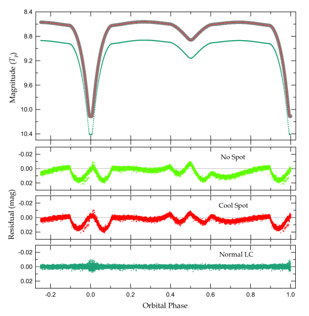
The orbital period () is equivalent to a frequency of = 1.0293088 0.0000005 day-1. Using this ephemeris, the phase-folded light curve of X Tri is presented in Figure 1.
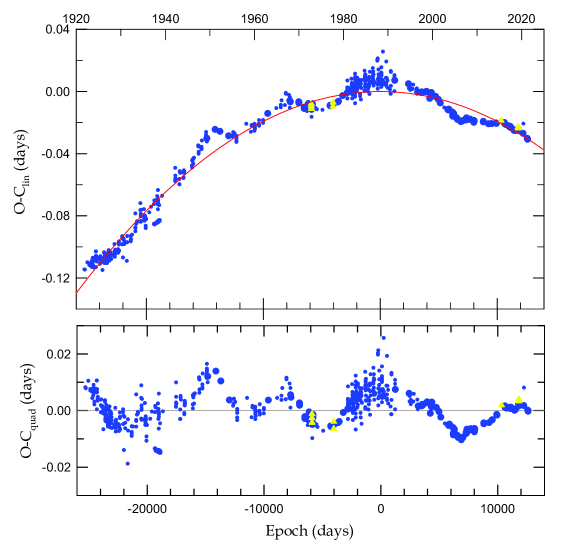
Using all available minimum epochs, we plotted the current eclipse timing diagram of X Tri, which is given in the upper panel of Figure 2. In this study we collected 653 times of minimum light. Most of the eclipse times can be found f.e. in the Gateway database222http://var2.astro.cz/ocgate/index.php?lang=en. The general trend of the values is a downward parabola, suggesting a long-term period decrease in this system. With the least-squares method, we derived the following quadratic ephemeris:
| (2) |
As was claimed by previous investigators, the secular period decrease cannot be connected with a mass transfer in the system. In case of a conservative mass transfer in such a semidetached system with the Roche-lobe filling secondary and more massive primary component, the orbital period should be increasing. The timing residuals from the quadratic ephemeris are presented in the lower panel. One can see irregular or quasi-periodic oscillations with typical lengths of about 20 years, which cannot be explained simply by a light-time effect (LITE) due to a circumbinary object. In this context, Liakos et al. (2010) suggested a multiple LITE of three additional bodies, which partially explain these variations.
X Tri is a member of a similar short-period Algol group (TU Her, FH Ori, TY Peg, Z Per, Y Psc) with a known long-term period decrease as well as short-period changes (Qian 2002). The nature of the long-term decrease as well as short-term irregular period changes has not yet been clearly and convincingly explained, and are often attributed to the mass and angular momentum loss mechanism, as developed by Tout & Hall (1991). Concerning a possible magnetic activity cycle in the secondary companion, there is not enough energy in the outer layers of the active cool star to reproduce the observed orbital period changes (Rovithis-Livaniou et al. 2000).
3 NEW SPECTROSCOPY AND DATA ANALYSIS
We conducted time-series spectroscopy through the BOES spectrograph mounted on the 1.8 m telescope at the Bohyunsan Optical Astronomy Observatory (Kim et al. 2007). Thirty-five spectra of X Tri were acquired on five nights between December 2019 and November 2020. Their wavelength range and resolving power are = 360010,200 and = 30,000, respectively. The integration time of the program target was set to 30 min, corresponding to 0.021 of the eclipse period. The raw CCD images were processed utilizing the IRAF packages CCDRED and ECHELLE. The reduction process was identical to that employed by Hong et al. (2015). The consequential signal-to-noise ratio (SNR) is approximately 40, measured between 4000 and 5000 .
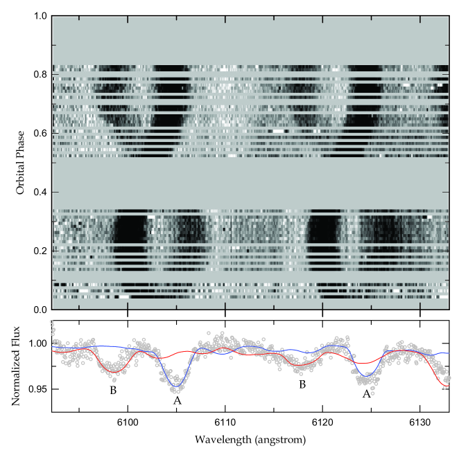
Struve (1946) reported that his results were not fully exempted from rotational broadening and line blending between the components. Trailed spectra are of great use to reveal and track the orbital motions of binary stars (e.g., Lee et al. 2018, 2020a,b). In order to look for sets of absorption lines for X Tri, we made the phase-folded trailed spectra from the BOES observations and examined them in detail at full wavelength. As a consequence, we found that Fe I 4957.61 and Ca I doublet 6103/6122 lines are strong enough to individually trace both component stars.
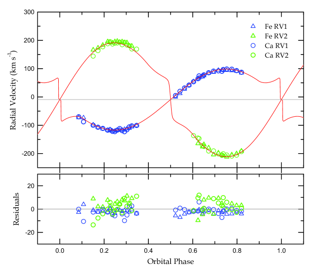
In Figure 3, the trailed spectra of the Ca I doublet are displayed in the upper panel and the spectrum observed on BJD 2,459,169.0452 (0.73 phase) is presented as an example in the lower panel. For RV determinations, the absorption lines were fitted several times by means of double Gaussian functions with the deblending routine in the IRAF task. The final RVs and their 1- values were averaged and standardized from these measurements. They are presented in Table 2 and Figure 4, where triangles and circles denote Fe I and Ca I RVs, respectively. From a sine-curve fit to each star’s RVs, we obtained the preliminary semi-amplitudes of = 107.8 km s-1 and = 202.2 km s-1, respectively, corresponding to a mass ratio of = 0.533.
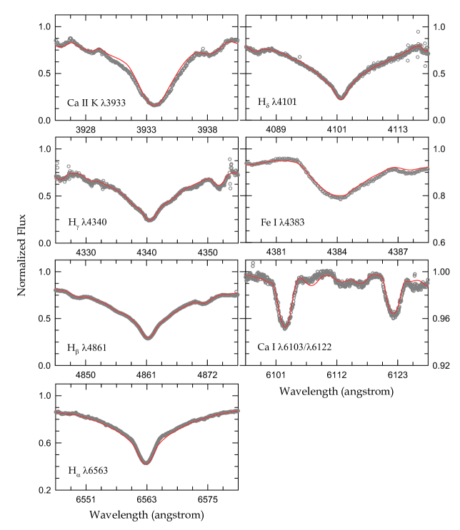
The atmospheric parameters of X Tri can be measured by comparing its observed spectra and synthetic models (Hong et al. 2017; Lee et al. 2022b). First of all, we constructed a disentangled spectrum from our BOES spectra and RV measures using the FDBinary code of Ilijić et al. (2004). Then, the projected rotational velocity () and effective temperature () of the primary component were yielded by minimizing the statistic between the reconstructed spectrum and model spectra. To do this, we generated grids of synthetic spectra in ranges of 10 200 km s-1 and 6000 10,000 K from the BOSZ spectral library (Bohlin et al. 2017). The surface gravity of = 4.3 (cf. Section 6) and the solar metallicity of Fe/H were applied to the calculations of the model spectra, because the two parameters are highly correlated with stellar temperatures. For the minimization, we selected seven spectral regions (Ca II 3933, Hδ 4101, Hγ 4340, Fe I 4383, Hβ 4861, Ca I doublet 6103/6122, Hα 6563), which are displayed in Figure 5. We acquired the best-fitting parameters of km s-1 and K. These values indicate that the primary star is rotating 1.7 times faster than Struve’s (1946) rate of 50 km s-1 and its spectral type is deduced to be A6.5 V (Pecaut & Mamajek 2013).
On the other hand, there is no evidence of any Balmer emission nor the presence of a circumstellar matter in our observed spectra. This may be because the emission feature is very weak and/or our SNR is not enough to detect it.
4 BINARY MODELING AND ABSOLUTE DIMENSIONS
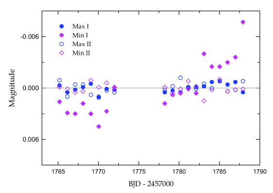
Like the historical data (Bozkurt et al. 1976; Liakos et al. 2010), the TESS light curve of X Tri has similarities to that of classical Algols. To see if there was any light variability in X Tri, we divided the time-series TESS data into 19 light curves at intervals of = 0.9715257 days and measured each of them at four orbital phases 0.0 (Min I), 0.25 (Max I), 0.5 (Min II), and 0.75 (Max II). These measurements appear in Table 3, where the BJD time of each segment is the middle of the beginning and the end. The average values at each phase are given in the last line of Table 3. As presented in this table, the primary eclipse depth is more than five times (1.24 mag) deeper than the secondary one and the depth difference implies a large temperature difference between the component stars. Further, Max I is 0.006 mag brighter than Max II, which may be indicative of stellar activities on and around both components. The light levels for each light curve were subtracted from the TESS average for the whole datasets and the mean residuals are plotted in Figure 6. We show that the primary minima gradually brightened up after the interruption in the middle point.
The TESS archive data and our velocity curves of X Tri were solved applying the Wilson-Devinney (W-D) code (Wilson & Devinney 1971, van Hamme & Wilson 2007) with the proximity and eclipse effects on RVs, as in the case of V404 Lyr (Lee et al. 2020a) and WASP 0131+28 (Lee et al. 2020b). The main difference between the 2007 version we used and the latest version is (1) direct distance estimation and (2) the use of absolute physical units (e.g., Kallrath, J. 2022), which does not affect our X Tri parameters. Thus, we used the 2007-version W-D code with features optimized by us, including repetitive routines. The absolute dimensions and distance determination of X Tri were calculated independently regardless of the W-D code.
In our synthesis, we fixed the primary’s temperature at K measured from the BOES spectra. It is assumed that X Tri A and B have predominately radiative and convective atmospheres, respectively. Bolometric albedo and gravity-darkening exponent were set to be (, ) = (1.0, 1.0) and (, ) = (0.5, 0.32). The logarithmic law was used for the limb-darkening effect (van Hamme 1993). Based on km s-1 and for the lobe-filling secondary, we adopted the rotation parameters of = 1.0 in the W-D synthetic code.
In a simultaneous light and RV solution, it is hard to assign reasonable weights to these observations. To resolve this, the binary modeling in this article was conducted in two steps. To begin with, the TESS light curve was analyzed using the value taken from our RV fitting. In the second, our RV curves were fitted by adopting the light curve parameters derived in the first step. Then again, the TESS data were analyzed applying the newly calculated spectroscopic elements (, , and ). This process was carried out for two cases without and with a starspot, and was repeated until both curves were reasonably solved.
Table 4 presents the final model parameters with a cool starspot located on the secondary’s surface, and the RV synthetic curves from them are shown as red lines in Figure 4. The red line in the top panel of Figure 1 presents our spot solution, and the light curve residuals corresponding to the unspotted and cool-spot models are given in the second and third panels. Although the light diminution seen between phases 0.5 and 0.8 was better described by the spot model, we could not fit the quasi-sinusoidal modulations to occur around both eclipses. The ‘W’-shape variation pattern of the residuals could result from some combination of stellar phenomena, such as magnetic activity, a gas stream from the lobe-filling component, and its impact on the detached companion. However, at present, we do not have a clear explanation for this puzzle. As in our previous studies (Lee et al. 2021, 2022a), the uncertainties of the binary star parameters in Table 4 were computed following the procedure applied by Southworth et al. (2020) for the TESS time-series data.
The binary star model indicates that X Tri is a semi-detached Algol, in which the detached primary component fills about 69 % of its inner Roche lobe. The absolute dimensions of each star in Table 5 were computed from the synthetic solution of the TESS data and our double-lined RVs. We used the solar magnitude of ⊙ = +4.73 and the empirical bolometric corrections (BCs) presented by Torres (2010). For measuring the distance to X Tri, we first obtained its apparent magnitude and color index (CI) to be = +9.01 0.02 and () = 0.28 0.03 mag, respectively, from the Tycho magnitudes of and (Høg et al. 2000). Then, the intrinsic CI of ()0 = +0.18 0.02 was estimated applying to the temperaturecolor calibration (Flower 1996), and () = +0.10 0.04. Our computed values lead to a nominal distance of 215 6 pc, which is in good agreement with 210 2 pc inverted from GAIA EDR3 ( = 4.753 0.042 mas; Gaia Collaboration et al. 2021).
5 PULSATIONAL CHARACTERISTICS
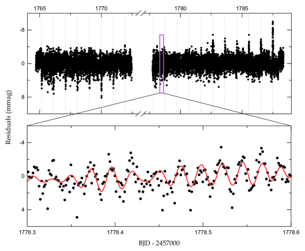
The fundamental parameters of X Tri in Table 5 indicate that the hotter primary star is present in the main-sequence (MS) Sct region of the Hertzsprung-Russell diagram, while the less massive secondary lies above the MS band where the lobe-filling companions of other semi-detached Algols exist (İbanoǧlu et al. 2006; Lee et al. 2016). Turner et al. (2014) found a pulsation period of 0.0220 0.0002 days in our target during their photometric survey to find eclipsing Sct stars. As displayed in the third panel of Figure 1, even our spot model did not fully explain the TESS light curve of X Tri with exceptional precision. It is not easy to extract reliable pulsating signals from the ‘W’-shape residuals. For useful multifrequency analyses, we made 1000 normal points phase-binning at intervals of 0.001. The mean light curve and the residuals from it are presented as the cyan dots in the top and bottom panels of Figure 1. The corresponding residuals distributed in BJD are given in Figure 7. We recognized that the binary signals were satisfactorily removed from the observed data and the primary eclipse depth varied with time.
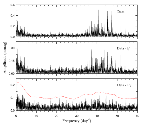
In order to investigate the oscillating features of X Tri, the PERIOD04 software by Lenz & Breger (2005) was introduced into the out-of-eclipse light curve residuals. The amplitude spectrum of the program target was calculated to the Nyquist frequency limit of 360 day-1. Using the pre-whitening technique (Lee et al. 2014), we found 16 significant signals with SNR larger than about 4 for each peak (Breger et al. 1993). The resultant frequency parameters are given in Table 6 and their uncertainties were obtained following Kallinger et al. (2008). The synthetic curve prepared from them appears as a solid line in Figure 7, and the periodogram of X Tri are presented in Figure 8. There are no conspicuous signals between 60 day-1 and .
As illustrated in Table 6 and Figure 8, the main signals of X Tri are distributed in the two frequency domains of 3 day-1 and 3652 day-1. Of our 16 frequencies, the highest amplitude signal corresponds to a frequency of 45.45 0.41 day-1 detected by Turner et al. (2014) within their errors, and appears to be the orbital harmonic of . We carefully explored combination frequencies within the Rayleigh frequency of = 0.042 day-1, from which our remarks are given in the last column of Table 6. We think the low frequencies below might be aliases or artefacts due to systematic trends. In contrast, most high frequencies may be identified as possible pulsation signals arising from the hotter and more massive primary.
6 DISCUSSION AND CONCLUSIONS
We have analyzed new spectroscopic observations of the semi-detached Algol X Tri with archival TESS data. The RV curves of the eclipsing pair were obtained by using the double Gaussian as a fitting function, and we measured the first RVs for the cool secondary star. The minimum method was applied to yield a rotational rate of km s-1 and a surface temperature of K for the primary star. With the atmospheric parameters, the TESS light and our RV curves let us characterize each binary component. From their simultaneous modeling, we determined the accurate masses and radii with less than 1% uncertainties, as follows: , , , and . For X Tri A, the synchronous rotation of = 86.7 0.5 km s-1 is well matched with our measurement of , unlike Struve’s (1946). At present, our program target is expected to be in a state of synchronous rotation. Meanwhile, X Tri is a semidetached Algol in which the less massive secondary fills the inner critical Roche lobe, while the more massive primary is detached and its fill-out factor is about 0.69. Thus, our target X Tri is a regular Algol, not a reverse Algol, i.e. the massive primary fills its Roche lobe.
Our binary synthesis revealed a third light of = 0.0374, which could originate from either circumbinary objects, as suggested by eclipse timing analyses, or other stars near X Tri because each pixel size of the TESS CCD camera is 21 arcsec on the sky (Ricker et al. 2015). There is a neighboring star TIC 28391715 (2MASS J02003411+2753233; Gaia EDR3 298268986033892480; = 12.007) with a separation of about 6.5 arcsec from our target star and a magnitude difference of 3.442 mag between them in the TESS passband. The brightness difference indicates that TIC 28391715 is about 24 times fainter than X Tri and hence contributes within 4 % of the total light. Thus, most of the source may be the nearby star TIC 28391715. The distance to TIC 28391715 is 207.6 0.7 pc from GAIA EDR3 parallax of 4.816 0.016 mas (Gaia Collaboration et al. 2021) and this is a good match to the Gaia distance 210 2 pc of X Tri. Further, the TESS targets seem to share a common proper motion; = 25.893 0.043 mas yr-1 and = 14.053 0.046 mas yr-1 for X Tri, and = 26.072 0.018 mas yr-1 and = 12.953 0.018 mas yr-1 for TIC 28391715. So then, TIC 28391715 may be gravitationally bound to the X Tri system, and the separation between them is estimated to be 1360 AU.
To extract more reliable oscillating frequencies, we formed a normal light curve at 0.001 phase intervals and the outside-eclipse residuals from it were applied to the PERIOD04 software package. Sixteen significant frequencies with SNR 4 were detected from the multifrequency analysis, of which the low frequencies in the gravity ()-mode domain are thought to be aliases or artefacts. Except for possible combinations within , our target star X Tri pulsates in the pressure ()-mode frequencies between 37 day-1 and 48 day-1 that originate from the primary star. The pulsation periods of the high frequencies are in the range of = 0.0210.027 days. Applying the Table 5 parameters to the relation of (Petersen & Jørgensen 1972), we obtained the pulsation constants of = 0.0140.018 days. The observed and values are typical of Sct oscillations (Breger 2000; Aerts et al. 2010). Thus, the detached primary component of X Tri is an oEA pulsator. Our pulsation data corresponding to the modes of Sct variables help to probe the stellar envelope of X Tri A through detailed asteroseismic modeling. However, it is difficult to probe the deep stellar interiors near the core region and to determine if there is a phase-dependence in these frequencies, because they did not detect in -mode pulsations and were observed in only a single TESS band.
Recently, Chen et al. (2022) found that three short-period binaries whose pulsations were discovered by TESS considerably exceed the upper limit of = 0.090.02, meaning that there is no correlation between them in these stars. X Tri has a relatively shorter orbital period than other normal oEA binaries (Mkrtichian et al. 2018). Its pulsation and orbital period ratios are . The physical parameters of our target star follow well the empirical relations of the , , and for the other oEA star with similiar orbital periods, where denotes the gravitational pulls onto the pulsating components exerted by companions (Soydugan et al. 2006; Liakos 2017; Liakos & Niarchos 2017). Also, our target exhibit almost the same pulsating characteristics as single Sct pulsators.
References
- Aerts et al (2010) Aerts, C., Christensen-Dalsgaard, J., & Kurtz, D. W. 2010, Asteroseismology (Dordrecht: Springer)
- Bohlin et al (2017) Bohlin, R. C., Mészáros, S., Fleming, S. W., et al. 2017, AJ, 153, 234
- Bowman et al (2019) Bowman, D. M., Johnston, C., Tkachenko, A., et al. 2019, ApJL, 883, L26
- Bozkurt et al (1976) Bozkurt, Ş., İbanoǧlu, C., Gülmen, Ö., & Güdür, N. 1976, A&AS, 23, 439
- Breger (2000) Breger, M. 2000, in ASP Conf. Ser. 210, Delta Scuti and Related Stars, ed. M. Breger and M. Montgomery (San Francisco: ASP), 3
- Breger et al (1993) Breger, M., Stich, J., Garrido, R., et al. 1993, A&A, 271, 482
- Chen et al (2022) Chen, X., Ding, X., Cheng, L., et al. 2022, ApJS, 263, 34
- Duchene & Kraus (2013) Duchêne, G., & Kraus, A. 2013, ARA&A, 51, 269
- Flower (1996) Flower, P. J. 1996, ApJ, 469, 355
- Frieboes-Conde & Herczeg (1973) Frieboes-Conde, H., & Herczeg, T. 1973, A&AS, 12, 1
- Gadomski (1932) Gadomski, J. 1932, Warsaw Univ. Reprint No. 15
- GAIA (2021) Gaia Collaboration, Brown, A. G. A., Vallenari, A., et al. 2021, A&A, 649, A1
- Høg (2000) Høg, E., Fabricius, C., Makarov, V. V., et al. 2000, A&A, 355, 27
- Hong et al (2015) Hong, K., Lee, J. W., Kim, S.-L., et al. 2015, AJ, 150, 131
- Hong et al (2017) Hong, K., Lee, J. W., Koo, J.-R., et al. 2017, AJ, 153, 247
- Ibanoǧlu et al (2006) İbanoǧlu, C., Soydugan, F., Soydugan, E., & Dervişoǧlu, A. 2006, MNRAS, 373, 435
- Ilijic et al (2004) Ilijić, S., Hensberge, H., Pavlovski, K., & Freyhammer, L. M. 2004, in ASP Conf. Ser. 318, Spectroscopically and Spatially Resolving the Components of the Close Binary Stars, ed. R. Hilditch, H. Hensberge, & K. Pavlovski (San Francisco: ASP), 111
- Kahraman Alicavus et al (2022) Kahraman Aliçavuş, F., Gümüş, D., Kirmizitaş, Ö., et al. 2022, RAA, 22, 085003
- Kahraman Alicavus et al (2017) Kahraman Aliçavuş, F., Soydugan, E., Smalley, B., & Kubát, J. 2017, MNRAS, 470, 915
- Kallinger et al (2008) Kallinger, T., Reegen, P., & Weiss, W. W. 2008, A&A, 481, 571
- Kallrath (2022) Kallrath, J. 2022, Galaxies, 10, 17
- Kim et al (2022) Kim, H.-Y., Hong, K., Kim, C.-H., et al. 2022, AJ, in press (arXiv:2209.09041)
- Kim et al (2007) Kim, K.-M., Han, I., Valyavin, G. G., et al. 2007, PASP, 119, 1052
- Kim et al (2003) Kim, S.-L., Lee, J. W., Kwon, S.-G., Youn, J.-H., Mkrtichian, D. E., & Kim, C. 2003, A&A, 405, 231
- Kwee & van Woerden (1956) Kwee, K. K., & van Woerden, H. 1956, BAN, 12, 327
- Lampens (2021) Lampens, P. 2021, Galaxies, 9, 28
- Lee et al (2021) Lee, J. W., Hong, K., & Kim, H.-Y. 2021, AJ, 161, 129
- Lee et al (2022a) Lee, J. W., Hong, K., Kim, H.-Y., & Park, J.-H. 2022a, MNRAS, 515, 4702
- Lee et al (2016) Lee, J. W., Hong, K., Kim, S.-L., & Koo, J.-R. 2016, MNRAS, 460, 4220
- Lee et al (2018) Lee, J. W., Hong, K., Koo, J.-R., & Park, J.-H. 2018, AJ, 155, 5
- Lee et al (2020a) Lee, J. W., Hong, K., Koo, J.-R., & Park, J.-H. 2020a, AJ, 159, 24
- Lee et al (2022b) Lee, J. W., Hong, K., & Park, J.-H. 2022b, MNRAS, 511, 654
- Lee et al (2014) Lee, J. W., Kim, S.-L., Hong, K., Lee, C.-U., & Koo, J.-R. 2014, AJ, 148, 37
- Lee et al (2020b) Lee, J. W., Koo, J.-R., Hong, K., & & Park, J.-H. 2020b, AJ, 160, 49
- Lee et al (2019) Lee, J. W., Kristiansen, M., & Hong, K. 2019, AJ, 157, 223
- Lenz & Breger (2005) Lenz, P., & Breger, M. 2005, Comm. Asteroseismology, 146, 53
- Liakos (2017) Liakos, A. 2017, A&A, 607, A85
- Liakos & Niarchos (2009) Liakos, A., & Niarchos, P. 2009, CoAst, 160, 2
- Liakos & Niarchos (2015) Liakos, A., & Niarchos, P. 2015, in ASP Conf. Ser. 496, Living Together: Planets, Host Stars and Binaries, ed. S. M. Rucinski, G. Torres, & M. Zejda (San Francisco: ASP), 195
- Liakos & Niarchos (2017) Liakos, A., & Niarchos, P. 2017, MNRAS, 465, 1181
- Liakos et al (2010) Liakos, A., Zasche, P., & Niarchos, P. 2010, in ASP Conf. Ser. 435, Binaries - Key to Comprehension of the Universe, ed. A. Prša, & M. Zejda (San Francisco: ASP), 101
- Mezzetti et al (1980) Mezzetti, M., Cester, B., Giuricin, G., & Mardirossian, F. 1980, A&AS, 39, 265
- Mkrtichian et al (2002) Mkrtichian, D. E., Kusakin, A. V., Gamarova, A. Y., et al. 2002, in ASP Conf. Ser. 256, Observational Aspects of Pulsating B- and A Stars, ed. C. Sterken, & D. W. Kurtz (San Francisco: ASP), 259
- Mkrtichian et al (2004) Mkrtichian, D. E., Kusakin, A. V., Rodriguez, E., et al. 2004, A&A, 419, 1015
- Mkrtichian et al (2018) Mkrtichian, D. E., Lehmann, H., Rodríguez, E., et al. 2018, MNRAS, 475, 4745
- Murphyz (2018) Murphy, S. J. 2018, preprint (arXiv:1811.12659)
- Neujmin (1922) Neujmin, G. 1922, AN, 217, 192
- Pecaut & Mamajek (2013) Pecaut, M. J., & Mamajek, E. E. 2013, ApJS, 208, 9
- Petersen & Jorgensen (1972) Petersen, J. O., & Jørgensen, H. E. 1972, A&A, 17, 367
- Qian (2002) Qian, S. 2002, PASP, 114, 650
- Rafert (1982) Rafert, J. B. 1982, PASP, 94, 485
- Ricker et al (2015) Ricker, G. R., Winn, J. N., Vanderspek, R., et al. 2015, JATIS, 1, 014003
- Rovithis-Livaniou et al (2000) Rovithis-Livaniou, H., Kranidiotis, A. N., Rovithis, P., & Athanassiades, G. 2000, A&A, 354, 904
- Shi et al (2022) Shi, X.-D., Qian, S.-B., & Li, L.-J. 2022, ApJS, 259, 50
- Soydugan et al (2006) Soydugan, E., İbanoǧlu, C., Soydugan, F., Akan, M. C., & Demircan, O. 2006, MNRAS, 366, 1298
- Struve (1946) Struve, O. 1946, ApJ, 104, 253
- Torres (2010) Torres, G. 2010, AJ, 140, 1158
- Tout & Hall (1991) Tout, C. A., & Hall, D. S. 1991, MNRAS, 253, 9
- Turner et al (2014) Turner, G., Katichuck, R., & Holaday, J. 2014, JAVSO, 42, 134
- Van Hamme (1993) Van Hamme, W. 1993, AJ, 106, 209
- Van Hamme & Wilson (1990) Van Hamme, W., & Wilson, R. E. 1990, AJ, 100, 198
- Van Hamme & Wilson (2007) Van Hamme, W., & Wilson, R. E. 2007, ApJ, 661, 1129
- Walker (1921) Walker, A. D. 1921, HarCi, 225, 1
- Wilson & Devinney (1971) Wilson, R. E., & Devinney, E. J. 1971, ApJ, 166, 605
- Wood (1950) Wood, F. B. 1950, ApJ, 112, 196
- Wood & Forbes (1963) Wood, B. D., & Forbes, J. E. 1963, AJ, 68, 257
- Zhang et al (2013) Zhang, X. B., Luo, C. Q., & Fu, J. N. 2013, ApJ, 777, 77
- Zhou (2010) Zhou, A. Y. 2010, arXiv:1002.2729v6
| BJD | Error | Min | BJD | Error | Min |
|---|---|---|---|---|---|
| 2,458,765.14863 | 0.00001 | I | 2,458,779.23707 | 0.00010 | II |
| 2,458,765.63585 | 0.00011 | II | 2,458,779.72151 | 0.00001 | I |
| 2,458,766.12013 | 0.00001 | I | 2,458,780.20852 | 0.00010 | II |
| 2,458,766.60747 | 0.00013 | II | 2,458,780.69301 | 0.00001 | I |
| 2,458,767.09168 | 0.00001 | I | 2,458,781.18010 | 0.00009 | II |
| 2,458,767.57895 | 0.00014 | II | 2,458,781.66456 | 0.00001 | I |
| 2,458,768.06322 | 0.00001 | I | 2,458,782.15148 | 0.00010 | II |
| 2,458,768.55024 | 0.00009 | II | 2,458,782.63613 | 0.00001 | I |
| 2,458,769.03474 | 0.00001 | I | 2,458,783.12299 | 0.00009 | II |
| 2,458,769.52184 | 0.00012 | II | 2,458,783.60761 | 0.00001 | I |
| 2,458,770.00627 | 0.00001 | I | 2,458,784.09455 | 0.00010 | II |
| 2,458,770.49336 | 0.00011 | II | 2,458,784.57913 | 0.00001 | I |
| 2,458,770.97779 | 0.00001 | I | 2,458,785.06601 | 0.00010 | II |
| 2,458,771.46491 | 0.00011 | II | 2,458,785.55067 | 0.00001 | I |
| 2,458,771.94933 | 0.00001 | I | 2,458,786.03754 | 0.00009 | II |
| 2,458,772.43605 | 0.00005 | II | 2,458,786.52221 | 0.00001 | I |
| 2,458,777.77844 | 0.00001 | I | 2,458,787.00902 | 0.00008 | II |
| 2,458,778.26567 | 0.00013 | II | 2,458,787.49374 | 0.00001 | I |
| 2,458,778.74997 | 0.00001 | I | 2,458,787.98039 | 0.00007 | II |
| Fe I 4957 | Ca I 6103 | |||||||||
|---|---|---|---|---|---|---|---|---|---|---|
| BJD | UT date | |||||||||
| (2,457,000+) | (km s-1) | (km s-1) | (km s-1) | (km s-1) | (km s-1) | (km s-1) | (km s-1) | (km s-1) | ||
| 1,820.0618 | 2019-12-02 | 6.1 | 2.2 | |||||||
| 1,820.0816 | 2019-12-02 | 4.4 | 6.2 | |||||||
| 1,820.1013 | 2019-12-02 | 4.9 | 6.3 | |||||||
| 1,820.1210 | 2019-12-02 | 5.9 | 6.7 | |||||||
| 1,820.1408 | 2019-12-02 | 7.6 | 5.0 | 8.5 | ||||||
| 1,820.1605 | 2019-12-02 | 5.6 | 10.0 | 7.7 | 10.7 | |||||
| 1,820.1803 | 2019-12-02 | 4.5 | 8.2 | 4.1 | 12.4 | |||||
| 2,145.1004 | 2020-10-22 | 8.8 | 6.7 | |||||||
| 2,145.1215 | 2020-10-22 | 7.4 | 11.9 | |||||||
| 2,145.2379 | 2020-10-22 | 6.4 | 9.0 | 7.0 | 6.7 | |||||
| 2,145.2590 | 2020-10-22 | 3.1 | 7.0 | 7.3 | 9.0 | |||||
| 2,145.2801 | 2020-10-22 | 4.5 | 4.5 | 5.3 | 5.5 | |||||
| 2,145.3013 | 2020-10-22 | 5.4 | 5.5 | 6.8 | 9.1 | |||||
| 2,145.3224 | 2020-10-22 | 6.8 | 8.2 | 4.3 | 5.3 | |||||
| 2,146.1355 | 2020-10-23 | 3.1 | 6.1 | 9.7 | 13.5 | |||||
| 2,146.1567 | 2020-10-23 | 6.4 | 6.8 | 5.4 | 10.2 | |||||
| 2,146.1778 | 2020-10-23 | 3.9 | 4.1 | 5.2 | 10.3 | |||||
| 2,146.1989 | 2020-10-23 | 5.4 | 9.6 | 4.5 | 8.5 | |||||
| 2,146.2201 | 2020-10-23 | 5.7 | 8.4 | 6.3 | 9.6 | |||||
| 2,146.2412 | 2020-10-23 | 5.0 | 5.5 | 4.2 | 7.2 | |||||
| 2,146.2623 | 2020-10-23 | 2.8 | 4.5 | 4.0 | 10.0 | |||||
| 2,146.2835 | 2020-10-23 | 5.0 | 5.1 | 5.2 | 7.6 | |||||
| 2,146.3046 | 2020-10-23 | 4.0 | 5.9 | 9.7 | 17.6 | |||||
| 2,146.3257 | 2020-10-23 | 2.6 | 5.6 | 7.8 | ||||||
| 2,167.0020 | 2020-11-13 | 3.4 | 5.6 | 16.9 | ||||||
| 2,167.0230 | 2020-11-13 | 3.0 | 9.8 | 5.2 | 17.1 | |||||
| 2,167.0441 | 2020-11-13 | 5.2 | 5.0 | 3.7 | 9.8 | |||||
| 2,167.0654 | 2020-11-13 | 5.4 | 6.6 | 6.0 | 9.1 | |||||
| 2,167.0868 | 2020-11-13 | 5.5 | 9.0 | 4.9 | 12.3 | |||||
| 2,167.1078 | 2020-11-13 | 4.5 | 7.3 | 6.7 | 8.7 | |||||
| 2,169.0452 | 2020-11-15 | 4.2 | 8.0 | 6.0 | 22.0 | |||||
| 2,169.0664 | 2020-11-15 | 5.0 | 7.8 | 6.5 | 9.6 | |||||
| 2,169.0883 | 2020-11-15 | 5.7 | 6.7 | 5.7 | 8.0 | |||||
| 2,169.1095 | 2020-11-15 | 3.0 | 8.2 | 7.1 | 8.2 | |||||
| 2,169.1308 | 2020-11-15 | 4.4 | 7.7 | 5.3 | 10.1 | |||||
| Mean Time | Min I | Max I | Min II | Max II |
|---|---|---|---|---|
| (BJD) | (mag) | (mag) | (mag) | (mag) |
| 2,458,765.17500 | 10.09720.0252 | 8.56520.0013 | 8.85620.0045 | 8.57080.0014 |
| 2,458,766.14726 | 10.09850.0275 | 8.56600.0014 | 8.85640.0040 | 8.57270.0020 |
| 2,458,767.11951 | 10.09860.0258 | 8.56570.0019 | 8.85680.0046 | 8.57130.0014 |
| 2,458,768.09176 | 10.09740.0263 | 8.56540.0024 | 8.85670.0039 | 8.57130.0013 |
| 2,458,769.06401 | 10.09860.0254 | 8.56500.0021 | 8.85540.0033 | 8.57250.0017 |
| 2,458,770.03626 | 10.10010.0268 | 8.56660.0011 | 8.85620.0036 | 8.57270.0011 |
| 2,458,771.00851 | 10.09830.0252 | 8.56560.0024 | 8.85570.0040 | 8.57200.0008 |
| 2,458,771.98006 | 10.09550.0265 | 8.56570.0019 | 8.85650.0034 | 8.57220.0008 |
| 2,458,778.22116 | 10.09740.0255 | 8.56600.0013 | 8.85620.0044 | 8.57190.0008 |
| 2,458,779.19340 | 10.09640.0254 | 8.56580.0006 | 8.85690.0042 | 8.57150.0016 |
| 2,458,780.16563 | 10.09620.0256 | 8.56600.0013 | 8.85640.0037 | 8.57050.0013 |
| 2,458,781.13787 | 10.09570.0262 | 8.56540.0010 | 8.85550.0026 | 8.57160.0017 |
| 2,458,782.11010 | 10.09620.0248 | 8.56540.0012 | 8.85610.0037 | 8.57180.0011 |
| 2,458,783.08232 | 10.09160.0260 | 8.56530.0012 | 8.85780.0033 | 8.57120.0010 |
| 2,458,784.05455 | 10.09310.0254 | 8.56480.0019 | 8.85650.0035 | 8.57170.0005 |
| 2,458,785.02678 | 10.09310.0257 | 8.56470.0010 | 8.85530.0025 | 8.57090.0008 |
| 2,458,785.99900 | 10.09260.0249 | 8.56510.0013 | 8.85670.0043 | 8.57210.0012 |
| 2,458,786.97122 | 10.09200.0258 | 8.56480.0007 | 8.85650.0042 | 8.57190.0009 |
| 2,458,787.90941 | 10.08790.0254 | 8.56600.0015 | 8.85640.0043 | 8.57090.0011 |
| Average | 10.09560.0031 | 8.56550.0005 | 8.85630.0006 | 8.57170.0006 |
| Parameter | Primary | Secondary |
|---|---|---|
| (BJD) | 2,458,765.1485970.000028 | |
| (day) | 0.97153190.0000018 | |
| () | 6.1050.021 | |
| (km s-1) | 9.210.29 | |
| (km s-1) | 108.150.50 | |
| (km s-1) | 209.830.98 | |
| 0.51540.0035 | ||
| (deg) | 88.900.14 | |
| (K) | 7900110 | 499050 |
| 4.2200.014 | 2.905 | |
| , | 0.673, 0.203 | 0.642, 0.165 |
| , | 0.5740.031, 0.214 | 0.6950.023, 0.188 |
| /(++) | 0.72100.0031 | 0.2416 |
| a | 0.03740.0024 | |
| (pole) | 0.26870.0013 | 0.30220.0011 |
| (point) | 0.27860.0015 | 0.43230.0013 |
| (side) | 0.27280.0013 | 0.31540.0012 |
| (back) | 0.27660.0014 | 0.34790.0012 |
| (volume)b | 0.27280.0014 | 0.32320.0012 |
| Spot Parameters: | ||
| Colatitude (deg) | 59.92.4 | |
| Longitude (deg) | 335.91.9 | |
| Radius (deg) | 16.82.8 | |
| spot/local | 0.8850.039 | |
| Parameter | Primary | Secondary |
|---|---|---|
| () | 2.1370.018 | 1.1010.010 |
| () | 1.6640.010 | 1.9720.010 |
| (cgs) | 4.3250.006 | 3.8900.006 |
| () | 0.4640.010 | 0.14390.002 |
| (km s-1) | 86.710.54 | 102.720.52 |
| (km s-1) | 846 | |
| (K) | 7900110 | 499050 |
| () | 9.670.55 | 2.160.09 |
| (mag) | 2.2670.062 | 3.8940.045 |
| BC (mag) | 0.0220.001 | 0.2920.017 |
| (mag) | 2.2450.062 | 4.1860.048 |
| Distance (pc) | 2156 | |
| Frequency | Amplitude | Phase | SNRb | Remark | |
|---|---|---|---|---|---|
| (day-1) | (mmag) | (rad) | |||
| 40.68400.0016 | 0.3220.062 | 1.550.57 | 8.86 | ||
| 45.22870.0010 | 0.4860.057 | 0.140.35 | 14.49 | ||
| 36.11390.0014 | 0.3200.054 | 1.150.49 | 10.16 | ||
| 43.51600.0014 | 0.3520.059 | 0.060.49 | 10.19 | ||
| 0.64020.0032 | 0.2530.095 | 5.561.10 | 4.57 | ||
| 37.30090.0017 | 0.2690.055 | 2.280.60 | 8.39 | ||
| 43.89750.0019 | 0.2660.059 | 2.100.64 | 7.78 | ||
| 45.29020.0015 | 0.3300.058 | 4.250.51 | 9.82 | ||
| 38.62360.0015 | 0.3210.056 | 2.740.51 | 9.76 | ||
| 51.82740.0017 | 0.2120.042 | 1.130.58 | 8.60 | ||
| 42.29500.0025 | 0.2090.063 | 1.110.88 | 5.72 | ||
| 0.95390.0041 | 0.1930.094 | 4.571.43 | 3.50 | ||
| 47.28910.0015 | 0.2980.054 | 5.470.53 | 9.43 | ||
| 2.09640.0036 | 0.2070.088 | 1.621.25 | 4.01 | ||
| 0.50660.0040 | 0.1980.094 | 6.061.39 | 3.61 | ||
| 39.77890.0034 | 0.1470.059 | 1.171.18 | 4.24 |