Abstract Orientable Incidence Structure and Algorithms for Finite Bounded Acyclic Categories. I. Incidence Structure

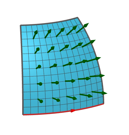
Below we will introduce incidence structure via parameterized $n$-dimensional surfaces, which are referred to as facets. Roughly speaking, a parameterized $n$-dimensional surface is a surface defined by a function of $n$ parameters. In order to rule out some strange geometries, some constraints are adopted. The points on the surface are described by the parameters called coordinates faithfully, so that the topological properties of this surface are fully described by the coordinate space. The coordinate space is not limit to an Euclidean space, so that it can describe non-trivial topology like torus. The values of coordinates are restricted to a given range in the coordinate space, which should be a compact and connected open subset. For example, the Figure 1 is a facet of a fragment of spherical shell described by $\{S(\theta,\phi)\mid 0<\theta<\pi/4,0<\phi<\pi/4\}$, where $S(\theta,\phi)\equiv\cos\theta\cos\phi\,\hat{x}+\sin\theta\cos\phi\,\hat{y}+\sin\phi\,\hat{z}$ is a point on the surface with coordinate $(\theta,\phi)$. The topology of this surface can be described by the coordinate range $(0,\pi/4)\times(0,\pi/4)\subset\mathbb{R}^{2}$. To describe a full sphere, the coordinate space cannot be an Euclidean space because it cannot faithfully refer to all points on the sphere. It is useful for doing actual geometric calculations if the coordinate space has a metric, which is important when it is not a Cartesian coordinate system. A good coordinate space should have small distortion, such that geometric calculations can be performed accurately. A cone can be described by $\{Y(x,y)|0<x^{2}+y^{2}<1\}$ with $Y(x,y)\equiv x\,\hat{x}+y\,\hat{y}+\,\sqrt{x^{2}+y^{2}}\hat{z}$, where the origin of the coordinate space $(0,0)$ has been removed since such point is not differentiable. This coordinate range is valid although it is not homeomorphic to a disk; there is no need to cut it off to make it homeomorphic to the disk. These examples shows how the flexibility of coordinate helps us to deal with real geometry more easily. As a special case, a point, described by a singleton set $\{P\}$, has a coordinate space with zero parameter, which is just a coordinate space that has only one valid coordinate.

If the coordinate space is orientable, the orientation of a facet can be defined. For convenience, we assume they are always orientable. The orientation of a facet at the point $F(u,v,\dots)$, denoted as $\hat{d}F(u,v,\dots)$, is defined as the normalization of the wedge product of the partial derivatives $dF(u,v,\dots)=\frac{\partial}{\partial u}F(u,v,\dots)\wedge\frac{\partial}{\partial v}F(u,v,\dots)\wedge\dots$. In the example of Figure 1, the orientation is $\hat{d}S(\theta,\phi)=\cos\theta\cos\phi\,\hat{y}\wedge\hat{z}+\sin\theta\cos\phi\,\hat{z}\wedge\hat{x}+\sin\phi\,\hat{x}\wedge\hat{y}$, which can be seen as a radial pseudovector. Each point in a $n$-dimensional facet has an orientation as a normalized multivector of degree $n$ (more precisely, a $n$-blade). In the same sense, the orientation of a line is just a multivector of degree 1, which is an unit tangent vector; the orientation of a point is just a multivector of degree 0, which only can be a sign. The orientation of a point cannot be derived naturally, so one should attach a sign to define its orientation, which is called a signed point.

A valid facet should be possible to be extended by including the boundary of the coordinate range, which is called closed facets. The image of the open coordinate range is called the inner of the facet, and the image of the boundaries of the coordinate range is called the boundaries of the facet. The inner and the boundaries of a facet should be disjoint. Unlike the inner of the facet, the boundaries are not faithfully described by coordinates, but are at least locally faithfully. To describe the boundaries of a given facet, a set of disjoint facets are introduced such that the union of them is equal to the boundaries, and these facets are called subfacets of the given facet. The relations between a facet and its subfacets are called incidence relations, which are described by embed function and local connectedness. Embed function is an mapping between coordinate spaces of facets, which shows how a facet is embedded into another one. For example, an arc $\{C(\theta)\mid 0<\theta<\pi/4\}$ with $C(\theta)\equiv\cos\theta\,\hat{x}+\sin\theta\,\hat{y}$ is covered by the surface of the example of Figure 1, which can be described by the equation $C(\theta)=S(\theta,0)$. This embed function is denoted as $\phi:C\to S$, where $C$ is a subfacet of the facet $S$. Notice that there can be multiple embed functions between two facets. For example, the circle, described by $\{C(\theta)|0<\theta<2\pi\}$ with $C(\theta)\equiv\cos\theta\,\hat{x}+\sin\theta\,\hat{y}$, covers the point $P\equiv 1\,\hat{x}+0\,\hat{y}$ in two ways: $P=C(0)$ and $P=C(2\pi)$. This is different from the conventional polytope, in which there is only one relation between incident facets.

The definiton of subfacets also implies two special facets. The null face $\varnothing$ is defined as an empty set, which has no valid coordinate. The null face is usually considered as a $(-1)$-dimensional facet. The null face $\varnothing$ is covered by all facets, because there is a map from an empty set to any set. Consider multiple disjoint facets with shared subfacets, the space containing these facets, called the universe $\mathbb{U}$, can also be considered as a facet. For example, 3D Euclidean space is defined as $\mathbb{U}(x,y,z)=x\,\hat{x}+y\,\hat{y}+z\,\hat{z}$. The universe $\mathbb{U}$ covers all facets because it is the codomain of functions defining facets. The null face $\varnothing$ and the universe $\mathbb{U}$ are called improper facets.

Another property of an incidence relation called the local connectedness is manifested by the relative position between two incident facets. If their dimensions differ by only $1$, the relative position can always be described by a sign (denoted as $|\phi|$), determining which the side of the subfacet faces the inner of the facet. In the example of Figure 1, the spherical shell is on the positive side of the arc according to the right-hand rule, so we define $|\phi|=+1$ (see Figure 1). Generalizing to incidence relation between $n$-dimensional and $(n{+}1)$-dimensional facets, we define the orientation between them as the difference of wedge products: if the $n$-dimentional subfacet $B$ is embedding into the $(n{+}1)$-dimentional facet $F$ by mapping $\phi:B\to F$, define $|\phi|$ as a sign such that $\hat{d}B\wedge\hat{n}=|\phi|\hat{d}F$, where $\hat{d}F$ and $\hat{d}B$ are their orientations at a point in the subfacet $B$, and $\hat{n}$ is a vector on this point pointing to the inner of the facet $F$. $|\phi|=+1$ ($|\phi|=-1$) means the subfacet $B$ is positively- (negatively-) oriented with respect to the facet $F$ (see Figure 2). Note that all points in the subfacet $B$ should give the same value of $|\phi|$. Under this definition, one can say: a line segment has one positive-oriented subfacet and one negative-oriented subfacet, and both of them are positive points at the endpoints; a circle with counter-clockwise tangent vectors is a positive-oriented subfacet of the enclosed disk; a sphere defined like the above example is negatively-oriented with respect to the enclosed ball. The incidence relation between the null face and a signed point is a special case: positive (negative) point always is positively- (negatively-) oriented with respect to the null face. A subfacet can be covered by a facet with multiple orientations. For example, consider a plane $S$ and a line segment $L$ which is in the middle of the plane. Since the plane is on the left and right of this line, there are two choices of the inward pointing vectors. Then the incidence relations between them are described by $\phi_{+}$ and $\phi_{-}$, which are the two identical embed functions with different orientations by letting $|\phi_{+}|=+1$ and $|\phi_{-}|=-1$.

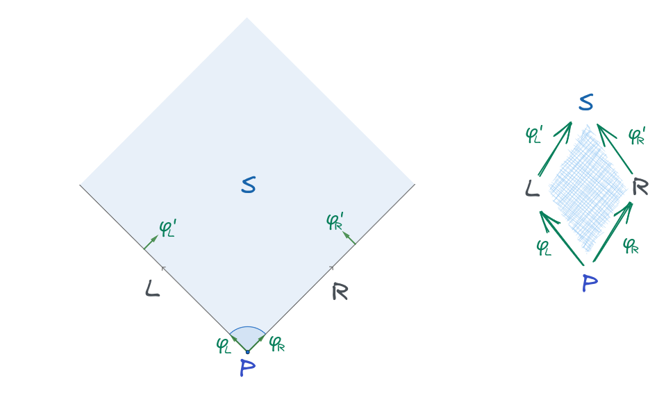
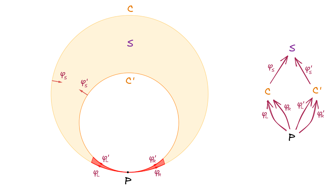
It is obviously that incidence relations are composable: if a point can embed into a line, and the line can embed into another surface, then this point can also embed into this surface. The equivalence relations between composed embed functions manifest the local connectedness, which is not just a sign. The incidence relations and their composition rules constitute an incidence structure. Figure 3 shows the incidence relations between a square and its vertex. The vertex point embeds into a square by mapping $\phi$, which is equal to composition $\phi_{L}^{\prime}\circ\phi_{L}$ and $\phi_{R}^{\prime}\circ\phi_{R}$, where $\phi_{L}$ ($\phi_{R}$) is the incidence relation from this point to the left (right) adjacent edge, and $\phi_{L}^{\prime}$ ($\phi_{R}^{\prime}$) is the incidence relation from the left (right) adjacent edge to the square. Such equivalence relation is just the diamond property in abstract polytope, and this property describes the completeness of the vertex. In abstract polytope, this diamond always exists and is unique for any two incident facets with dimension differing by $2$. If there is a shape that has two vertices sharing the same point, this point is covered by this area in two directions. For example, consider the area between two internally tangent circles called crescent shape (see Figure 4), the tangent point is covered by outer circle in two directions, say $\phi_{L}$ and $\phi_{R}$, and outer circle is also covered by the crescent shape, say $\phi_{S}$. Then one can go from the tangent point to the inner of the crescent shape in two ways, which is equal to $\phi_{S}\circ\phi_{L}$ and $\phi_{S}\circ\phi_{R}$. These two incidence relations are not equivalent, so they don’t form a diamond; the angle between these two edges has been separated by the inner circle. Instead, the diamonds are formed by $\phi_{S}\circ\phi_{L}=\phi_{S}^{\prime}\circ\phi_{L}^{\prime}$ and $\phi_{S}\circ\phi_{R}=\phi_{S}^{\prime}\circ\phi_{R}^{\prime}$, where $\phi_{L}^{\prime}$, $\phi_{R}^{\prime}$ and $\phi_{S}^{\prime}$ are the same as above but relative to the inner circle. These two diamonds represent two different directions of incidence relations between the tangent point and the crescent shape; there are two separated ranges of angles that can go from this point to the inner. It shows the difference between diamonds indicates the local connectedness around the point.

Not all incidence relations can be defined continuously. The Riemann surface $R(z)\equiv(z,f(z))$ for the function $f(z)=\sqrt{z}(1-|z|)$ with $0<|z|<1$ is a $2$-dimensional facet in a $4$-dimensional space, which doubly cover the unit circle $C(z)\equiv(z,0)$ with $|z|=1$. Their are two incidence relations: any point on the circle, say $C(e^{i\theta})$, should be mapped to $R(e^{i\theta})$ and $R(e^{i(2\pi+\theta)})$, representing two embed functions respectively. Depending on the choice of the branch cut, the embed functions are discontinuous at that point. It is impossible to write such embed functions as continuous functions. Breaking of continuity may cause some geometric calculation problems. To solve this problem, the calculation should be limited to a small range, such that in this range the embed functions can be written as continuous functions depending on where it is. A facet with a non-orientable subfacet will also encounter similar problems, in which the incidence relations cannot have a continuous sign. These kind of incidence relations are said to be non-orientable. To simplify the discussion, we only focus on the incidence structure with orientable incidence relations, which we call an orientable incidence structure.

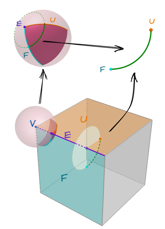
To explain the concept of local connectedness more clearly, we shall introduce vertex figures, which is defined in the same manner as polytope. To make a vertex figure on a $0$-dimensional facet (a positive point), one puts a ball $D^{n}$ on it, which is small enough so that only the facets that cover this point intersect this ball. Then the sliced images of facets (the intersection of the boundary of the ball $\partial D^{n}$ and facets) are defined as the vertex figure of the corresponding facets. For example, the vertex figure on a vertex of a cube is a spherical triangle, which is an intersection of the cube and a sphere centered at this vertex (see Figure 5). The orientation of the sliced image $L$ of the facet $F$ should obey $\hat{n}\wedge\hat{d}L=\hat{d}F$, where $\hat{n}$ is outward pointing vector from the center of the slicing ball. The incidence relations of this vertex figure can be trivially derived by restricting the domain and codomain of mapping. It’s easy to prove that the sign of incidence relations are the same. More general, the vertex figure on any facet can be defined as: pick a point on given $m$-dimensional facet $V$, and put a ball $D^{n-m}$ on this point, which is perpendicular to its orientation $\hat{d}V$ at this point. Then the sliced images of facets (the intersections of the boundary of this ball $\partial D^{n-m}$ and facets) are defined as the vertex figure of the corresponding facets on the facet $V$. All points on the facet $V$ should give the same vertex figure. The orientation of the sliced image $L$ of the facet $F$ should obey $\hat{d}V\wedge\hat{n}\wedge\hat{d}L=\hat{d}F$, where $\hat{n}$ is outward pointing vector from the center of the the slicing ball. For example, the vertex figure on an edge (i.e., the edge figure) of a cube is a segment of arc, which is the intersection of the cube and a circle with this edge as its axis (see Figure 5). Its obviously the operations of taking vertex figure are composable. For example, the edge figure of a cube is the vertex figure of the vertex figure, as shown in Figure 5.

Some sliced images on a subfacet have multiple connected components, each of them is defined as an individual facet in this vertex figure. This kind of facets are said to be locally separated by this subfacet. For example, the vertex figure of a plane on a point lying in the middle of the plane is a circle, which is connected, so we say the plane is not locally separated by this point. But the vertex figure of a plane on a line lying in the middle of the plane becomes two points, which have two connected components, so we say the plane is locally separated by this line. The crescent shape (Figure 4) is a non-trivial example, whose vertex figures on the tangent point are two line segments, so we say the crescent shape is locally separated by the tangent point. It shows the local connectedness property described by incidence relation becomes connectedness property of the vertex figure, and such correspondence is naturally required if one considers the incidence structure of the vertex figure. Also, the local connectedness property can be propagated via connectivity, so incidence relations can be tested in every points in the connected subfacet. These descriptions manifest the local and global properties of incidence relations.

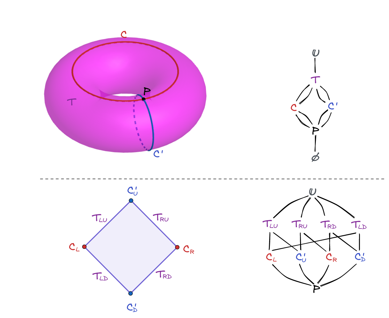
The orientable incidence structure can be drawn as directed acyclic multigraphs, where nodes are facets, and edges are nondecomposable embed functions. In this diagram, called the Hasse diagram, all incident facets can be connected by directed paths, manifesting the poset structure of incidence relations. The Hasse diagram is not enough to describe an orientable incidence structure, since the composition rules for incidence relations are not shown. Because sliced images of connected facets may become disconnected, the incidence structure of a vertex figure is not just a subgraph of the Hasse diagram. For example, the vertex figure on the intersection point of two circles on a torus is much more complicated to itself (see Figure 6), but the composition rules of incidence relations are always the same.

In our theory, the incidence relations are not unique to two incident facets. The difference of two incidence relations represents the local connectedness of the facet, which is the main difference to the conventional incidence structure. The existence of multiple incidence relations forces us to consider the composition rules between them. Unlike abstract polytope, where the structure can be described by a poset, the orientable incidence structure act like a category. We will extract out such structure in the next section.

The abstract orientable incidence structure is an algebraic structure which represents the orientable incidence relations between facets. Unlike previous section, it only captures its combinatorial nature without specifying geometric properties. An abstract orientable incidence structure, denoted as $\mathcal{F}$, is a graded bounded acyclic category satisfying semi-diamond property. An acyclic category is a category without non-trivial cycles. It is impossible to have two non-identity morphisms in opposite directions at the same time, so morphisms can only go in one direction. For a finite acyclic category, there is a rank function that maps an object to an integer, so that all morphisms increase the rank of object except identity. One can define the rank of an object as the dimension of corresponding facet. The acyclic category with a rank function is called graded acyclic category. Bounded means it has exactly one initial object and terminal object. The initial object, which has the lowest rank, represents the null face, denoted as $\varnothing$; the terminal object, which has the highest rank, represents the universe, denoted as $\mathbb{U}$. Morphisms represent incidence relations between the facets. The morphism $\phi:F\rightarrow S$ means that facet $F$ is covered by facet $S$. There may have multiple morphisms between two objects, and this property represents the local connectedness of the incidence relation, as we discussed above. Below we mainly focus on the property of bounded acyclic category, and compare it with the bounded poset.

Recall the definition of a bounded poset (a poset which includes its lower and upper bounds), which is the base of abstract polytope:

1. 1.

   irreflexivity: $a\nless a$.

2. 2.

   asymmetry: if $a<b$ then $b\nless a$.

3. 3.

   transitivity: if $a<b$ and $b<c$ then $a<c$.

4. 4.

   least: there exists exactly one $\varnothing$ such that forall $a\neq\varnothing$ there is $\varnothing<a$.

5. 5.

   greatest: there exists exactly one $\mathbb{U}$ such that forall $a\neq\mathbb{U}$ there is $a<\mathbb{U}$.

Now compare to the definition of bounded acyclic category:

1. 1.

   irreflexivity: there is no $\phi:F\rightarrow F$ for any $\phi\neq\operatorname{id}$.

2. 2.

   asymmetry: if there is $\phi:F\rightarrow S$ for some $\phi\neq\operatorname{id}$, then there is no $\phi^{\prime}:S\rightarrow F$ for any $\phi^{\prime}\neq\operatorname{id}$.

3. 3.

   transitivity: if there are $\phi:P\rightarrow F$ and $\phi^{\prime}:F\rightarrow S$ for some $\phi\neq\operatorname{id}$ and $\phi^{\prime}\neq\operatorname{id}$, then $\phi^{\prime}\circ\phi:P\rightarrow S$.

4. 4.

   initial: there exists exactly one $\varnothing$, such that forall $F\neq\varnothing$ there is $\phi:\varnothing\rightarrow F$ for exactly one $\phi\neq\operatorname{id}$.

5. 5.

   terminal: there exists exactly one $\mathbb{U}$, such that forall $F\neq\mathbb{U}$ there is $\phi:F\rightarrow\mathbb{U}$ for exactly one $\phi\neq\operatorname{id}$.

The key different is that, there can be multiple relations between two objects in the bounded acyclic category, and the transitivity of order relations becomes the composition of morphisms. A bounded poset is just a thin bounded acyclic category. It is natural to define an induced bounded poset for a bounded acyclic category by forgetting differences between multiple relations. In this sense, one says acyclic category is a generalization of poset. Abstract orientable incidence structure also loosens three constraints of abstract polytope, which will be discussed in the end of this section. Notice that the rules least and greatest in a bounded poset becomes initial and terminal, which looks stricter in the bounded acyclic category. The initial object and the terminal object are called improper objects.

The upper closure of an element $x$ in a bounded poset $\mathcal{P}$ is a subset whose element is greater than or equal to $x$. Such subset is also a bounded poset, where the order relation is inherited from the host poset $\mathcal{P}$. To emphasize this, it is denoted as $\mathcal{P}\operatorname{\uparrow}x$. Similarly, one can construct a full subcategory $\mathcal{F}^{\prime}$ by only including the upper closure of an object $F_{m}$. There is no non-trivial morphism that point to the object $F_{m}$, but it is not an initial object since the morphism $\phi:F_{m}\to S$ may not be unique for the object $S$, so that it is not a bounded acyclic category. To fix it, one should split objects such that there is only one initial morphism for each object. Construct upper category of object $F_{m}$ in a bounded acyclic category $\mathcal{F}$, denoted as $\mathcal{F}\operatorname{\uparrow}F_{m}$: $\operatorname{Obj}(\mathcal{F}\operatorname{\uparrow}F_{m})$ is a set of $F_{s}|\phi_{sm}\rangle$ for all objects $F_{s}$ and morphisms $\phi_{sm}:F_{m}\rightarrow F_{s}$. $\operatorname{Hom}(F_{s}|\phi_{sm}\rangle,F_{t}|\phi_{tm}\rangle)$ is a set of $\phi_{ts}|\phi_{sm}\rangle:F_{s}|\phi_{sm}\rangle\rightarrow F_{t}|\phi_{tm}\rangle$ for all morphisms $\phi_{ts}:F_{s}\rightarrow F_{t}$ and $\phi_{sm}:F_{m}\to F_{s}$ such that $\phi_{ts}\circ\phi_{sm}=\phi_{tm}$. The composition rule is $\phi_{pt}|\phi_{tm}\rangle\circ\phi_{ts}|\phi_{sm}\rangle=\phi_{ps}|\phi_{sm}\rangle$ with $\phi_{ps}=\phi_{pt}\circ\phi_{ts}$. The object $F_{t}$ have been marked with morphism $\phi_{tm}$, so that it is splitted into multiple objects corresponding to each initial morphism $\phi_{tm}$. Although the object splits, the composition rule is inherited from the host category $\mathcal{F}$. In terms of incidence structure, the upper category $\mathcal{F}\operatorname{\uparrow}F_{m}$ just corresponds to the vertex figure on an object $F_{m}$: in upper category, an object $F_{n}|\phi_{nm}\rangle$ represents a connected component of sliced images, and a morphism $\phi_{ts}|\phi_{sm}\rangle$ represents an incidence relation between facets $F_{s}|\phi_{sm}\rangle$ and $F_{t}|\phi_{tm}\rangle$.

There is a functor $F_{m}^{\downarrow}:\mathcal{F}\operatorname{\uparrow}F_{m}\rightarrow\mathcal{F}$ that maps object $F_{s}|\phi_{sm}\rangle$ to $F_{s}$, and maps morphism $\phi_{ts}|\phi_{sm}\rangle:F_{s}|\phi_{sm}\rangle\rightarrow F_{t}|\phi_{tm}\rangle$ to $\phi_{ts}:F_{s}\rightarrow F_{t}$. This functor is a reversed operation of taking upper category, so it is named downward functor. Drawn as Hasse diagrams, the downward functor becomes graph homomorphism between two graphs. Unlike the abstract polytope, this is not injective on nodes and edges, which manifests the local connectedness of incidence relations.

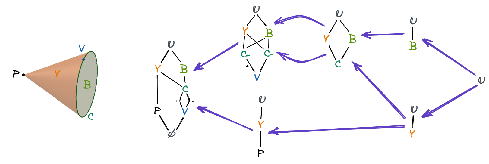
Since an upper category itself is also a bounded acyclic category, one can further construct an upper category of an object in the upper category. The category $\mathcal{F}\operatorname{\uparrow}F_{m}\operatorname{\uparrow}F_{n}|\phi_{nm}\rangle$ is an upper category of object $F_{n}|\phi_{nm}\rangle$, where $\operatorname{Obj}(\mathcal{F}\operatorname{\uparrow}F_{m}\operatorname{\uparrow}F_{n}|\phi_{nm}\rangle)$ is a set of object $F_{s}|\phi_{sm}\rangle|\phi_{sn}|\phi_{nm}\rangle\rangle$, or abbreviated as $F_{s}|\phi_{sn},\phi_{nm}\rangle$, for all objects $F_{s}$ and morphisms $\phi_{sn}:F_{n}\rightarrow F_{s}$; $\operatorname{Hom}(F_{t}|\phi_{tn},\phi_{nm}\rangle,F_{s}|\phi_{sn},\phi_{nm}\rangle)$ is a set of $\phi_{ts}|\phi_{sm}\rangle|\phi_{sn}|\phi_{nm}\rangle\rangle:F_{s}|\phi_{sm}\rangle|\phi_{sn}|\phi_{nm}\rangle\rangle\rightarrow F_{t}|\phi_{tm}\rangle|\phi_{tn}|\phi_{nm}\rangle\rangle$, or abbreviated as $\phi_{ts}|\phi_{sn},\phi_{nm}\rangle:F_{s}|\phi_{sn},\phi_{nm}\rangle\rightarrow F_{t}|\phi_{tn},\phi_{nm}\rangle$ for all morphisms $\phi_{ts}:F_{s}\rightarrow F_{t}$ and $\phi_{sn}:F_{n}\rightarrow F_{s}$ such that $\phi_{ts}\circ\phi_{sn}=\phi_{tn}$. Noting that we assume $\phi_{sm}=\phi_{sn}\circ\phi_{nm}$ and $\phi_{tm}=\phi_{tn}\circ\phi_{nm}$, and the abbreviation works because $\phi_{sm}$ can be determined uniquely. It is isomorphic to the upper category $\mathcal{F}\operatorname{\uparrow}F_{n}$, which shows that taking upper category is composable. This rule is consistent with above discussion: taking vertex figure is composable. Similarly, downward functors are also composable. Downward functor can be reduced down to a functor $\phi_{mn}^{\downarrow}:\mathcal{F}\operatorname{\uparrow}F_{m}\rightarrow\mathcal{F}\operatorname{\uparrow}F_{n}$ for morphism $\phi_{mn}:F_{n}\rightarrow F_{m}$, in which object $F_{s}|\phi_{sm}\rangle$ is mapped to $F_{s}|\phi_{sn}\rangle$, and morphism $\phi_{ts}|\phi_{sm}\rangle:F_{s}|\phi_{sm}\rangle\rightarrow F_{t}|\phi_{tm}\rangle$ is mapped to $\phi_{ts}|\phi_{sn}\rangle:F_{s}|\phi_{sn}\rangle\rightarrow F_{t}|\phi_{tn}\rangle$, where $\phi_{sn}=\phi_{sm}\circ\phi_{mn}$. Upper closures of a poset form a poset by inclusion relation, its opposite category is isomorphic to the host poset. Similarly, upper categories $\{\mathcal{F}\operatorname{\uparrow}F_{m}|F_{m}\in\operatorname{Obj}\}$ and downward functors $\{\phi_{mn}^{\downarrow}|\phi_{mn}\in\operatorname{Hom}\}$ also form a bounded acyclic category, its opposite category is isomorphic to the host category $\mathcal{F}$ (see Figure 7).

The Hasse diagram of a bounded acyclic category can easily see which part is splittable. Two proper objects are said to be linked if they are connected in the Hasse diagram excluding improper objects. If not all proper objects are linked, this category is said to be splittable. It is the generalization of connectedness condition of abstract polytope. The linked objects may form multiple clusters, and they can be splitted into separated bounded acyclic categories. The linked clusters can be determined by linkages between minimal/maximal objects, which are defined as minimal/maximal elements of the induced poset of all proper objects. A bounded acyclic category is said to be strongly unsplittable iff all sections are unsplittable, which is an analogue of strongly connectedness of posets. The definition of sections in an acyclic category will be introduced latter. The words “linked” and “splittable” are used because “disjoint” and “disconnected” are reserved for actual geometric properties.

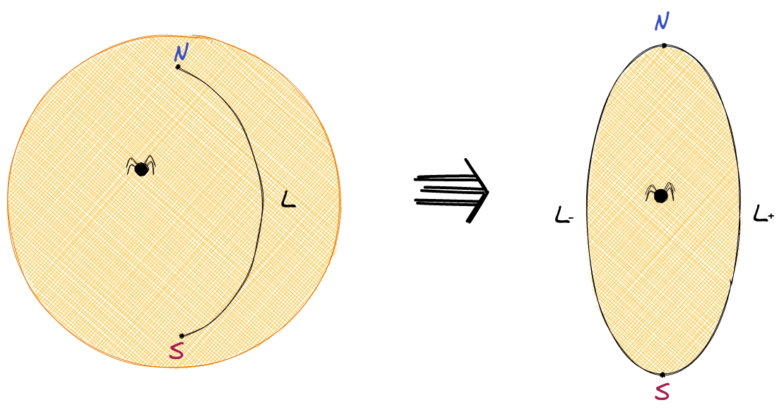
There is a dual concept of upper category called lower category, which is a generalization of lower closure of a poset. Upper category is constructed by treating one object as the initial object, and split objects such that outgoing morphisms are initial morphisms. In the opposite, lower category, denoted as $\mathcal{F}\operatorname{\downarrow}F_{m}$, is constructed by treating one object as the terminal object, and split objects such that incoming morphisms are terminal morphisms: $\operatorname{Obj}(\mathcal{F}\operatorname{\downarrow}F_{m})$ is a set of $\langle\phi_{mt}|F_{t}$ for all objects $F_{t}$ and morphisms $\phi_{mt}:F_{t}\rightarrow F_{m}$; $\operatorname{Hom}(\langle\phi_{ms}|F_{s},\langle\phi_{mt}|F_{t})$ is a set of $\langle\phi_{mt}|\phi_{ts}:\langle\phi_{ms}|F_{s}\rightarrow\langle\phi_{mt}|F_{t}$ for all morphisms $\phi_{ts}:F_{s}\rightarrow F_{t}$ and $\phi_{mt}:F_{t}\rightarrow F_{m}$ such that $\phi_{mt}\circ\phi_{ts}=\phi_{ms}$. The composition rule is $\langle\phi_{mp}|\phi_{pt}\circ\langle\phi_{mt}|\phi_{ts}=\langle\phi_{mp}|\phi_{ps}$ with $\phi_{ps}=\phi_{pt}\circ\phi_{ts}$. In geometry, lower category corresponds to face figure, which is like imagining an ant living in a 2D world. The face figure of a sphere with one meridian is equivalent to a 2D space bounded by two lines (see Figure 8). The line is duplicated because it is covered by the sphere in two ways. As a creature living in 3D space, we know it is one line, but for the 2D creatures living on the sphere, they only see a space rift, and they cannot confirm if there is a wider space in this rift.

There is also a categorical analogue of the interval of a poset: $[a,b]\equiv\{c\in\mathcal{P}|a\leq c\leq b\}$, which can be seen as a lower closure of an upper closure. Given a poset, by taking non-trivial intervals between all minimal and maximal elements, the given poset can be covered by multiple bounded posets. Similarly, an acyclic category can be turned into direct sum of bounded acyclic categories by splitting objects, and those bounded acyclic categories are called sections, whose name comes from abstract polytope. Consider an acyclic category, say $\mathcal{F}$, define a section category of morphism $\phi_{0}$ on $\mathcal{F}$, denoted as $\langle\mathcal{F}\rangle_{\phi_{0}}$: $\operatorname{Obj}(\langle\mathcal{F}\rangle_{\phi_{0}})$ is a set of $\langle\phi_{n}^{\ast}|\phi_{n}\rangle$ for all morphisms $\phi_{n}^{\ast}$ and $\phi_{n}$ such that $\phi_{n}^{\ast}\circ\phi_{n}=\phi_{0}$. $\operatorname{Hom}(\langle\phi_{n}^{\ast}|\phi_{n}\rangle,\langle\phi_{m}^{\ast}|\phi_{m}\rangle)$ is a set of $\langle\phi_{m}^{\ast}|\phi_{mn}|\phi_{n}\rangle$ for all morphisms $\phi_{m}^{\ast}$, $\phi_{mn}$, $\phi_{n}$ such that $\phi_{m}^{\ast}\circ\phi_{mn}\circ\phi_{n}=\phi_{0}$.

taking section category doesn’t break the algebra of morphisms, it just renames some objects so that it is bounded. “The algebra of morphisms” is the generalization of “the transitivity of order relation”. Define local-embedding function for a poset: an order-preserving function $f$ is local-embedding iff it is an order isomorphism between $[x,y]$ and $[f(x),f(y)]$ for any pair $x\leq y$. That is, the element $f(x)\leq z^{\prime}\leq f(y)$ implies there exists exactly one $x\leq z\leq y$ such that $f(z)=z^{\prime}$. Note that it is not an one-to-one function. The generalization to an acyclic category becomes a local-embedding functor: for any morphism $\phi$, the pair of morphisms $\psi^{\prime}$ and $\psi^{\prime\prime}$ with constraint $\psi^{\prime\prime}\circ\psi^{\prime}=\mu(\phi)$ implies there exists exactly one pair of morphisms $\phi^{\prime}$ and $\phi^{\prime\prime}$ with constraint $\phi^{\prime\prime}\circ\phi^{\prime}=\phi$ such that $\mu(\phi^{\prime})=\psi^{\prime}$ and $\mu(\phi^{\prime\prime})=\psi^{\prime\prime}$. The inverse of taking section categories is the local-embedding functor. Local-embedding functor describes the correspondence of algebra of morphisms without mention any object. It shows that the identity of object isn’t important in a bounded acyclic category; initial morphisms and terminal morphisms are enough to indicate objects in a bounded acyclic category.

The chain representation provides a clear view of this. Recall the definition of the chain of a poset, which is defined as a total ordering subset. A subset of a chain is also total ordering, called a subchain. In an acyclic category, the morphism between two objects is not unique, so the generalization becomes: the morphism chain of a morphism $\phi_{n0}:F_{0}\rightarrow F_{n}$ is a non-empty sequence of morphisms $\langle\phi_{n},\dots,\phi_{2},\phi_{1}\rangle$ that composed to this morphism. Its subchain can be constructed by composing adjacent morphisms into one. In other words, a subchain just skips some intermediate objects except the start and end, which is slightly different from the conventional definition of the morphism chain. A morphism chain containing identity morphisms is said to be degenerated. A morphism chain with $n$ intermediate object is called $n$-chain. $0$-chain is just the host morphism itself $\langle\phi_{n0}\rangle$, so it is said to be a trivial chain. $1$-chain represents an object of the section of the morphism $\phi_{n0}$, and $2$-chain represents a morphism, whose source object and target object are just two non-trivial subchains.

Abstract orientable incidence structure can be described by only their subchain relations, called a nerve, which is also slightly different from the conventional definition. The nerve of an acyclic category is composed by a collection of $n$-chains $N_{n}=\{\langle\phi_{n},\dots,\phi_{1},\phi_{0}\rangle\}$ for $n=0,1,2,\dots$ and the face maps $d_{i}:N_{n}\to N_{n-1}$ for $i=1\sim n$, which skip the $i$-th object in the $n$-chain, and the degeneracy maps $s_{i}:N_{n}\to N_{n+1}$ for $i=1\sim n$, which insert an identity morphism at the $i$-th object. The laws for face maps and degeneracy maps are the same as the conventional one, which should not be repeated here. Note that in our definition, a $1$-chain represents an object, not a morphism. A bounded acyclic category has nerve with only one $0$-chain, which will back to the conventional definition by replacing $n$ with $n-1$. The upper category of a $1$-chain $F$ becomes easy to define in this formulation, which is just letting $N_{n}^{\prime}=d_{1}^{-n}(F)$ and $d_{i}^{\prime}=d_{i}$, $s_{i}^{\prime}=s_{i}$, where $d_{1}^{-n}$ indicates taking preimage of $d_{1}$ $n$ times. Lower category and section category can be defined in a similar approach. Two acyclic categories will have the same nerve if they are surjectively section-embedded by the same direct sum of bounded acyclic categories. Because no relabeling is required, nerves are more natural for describing orientable incidence structures.

A section category not only can be defined on an acyclic category, but also on the non-recursive category, which is a category without non-trivial non-degenerated recursive morphism chain, that is, $\psi\circ\phi\circ\psi^{\prime}=\phi$ implies $\psi$ and $\psi^{\prime}$ being identity morphisms. This property only rules out the infinity of morphisms, and non-trivial cycles of morphisms are still possible, while ensuring that their section categories are bounded acyclic categories. Non-recursiveness and finiteness naturally induce acyclicity.

The diamond property of an abstract orientable incidence structure is stated as: a 2-rank morphism should be divided into exactly two maximum chains. 2-rank morphism means the rank of source object and target object differ by 2. In other words, a $1$-dimensional facet should have exactly 2 $0$-dimensional subfacets, that means only line segments are valid $1$-dimensional facets. Moreover, the multiplication of the sign of chains should be different, that is, a valid diamond should obey $\phi_{+}\circ\psi_{+}=\phi_{-}\circ\psi_{-}$ and $|\phi_{+}|\times|\psi_{+}|=-|\phi_{-}|\times|\psi_{-}|$. This property captures the topological nature of the Euclidean space. To include infinite lines and rays as valid $1$-dimensional facets, this property should be loosen. The semi-diamond property can be stated as: a 2-rank morphism can be divided into at most two maximum chains. In other words, a $1$-dimensional facet should have at most 2 $0$-dimensional subfacets.

Except diamond property, the conventional abstract polytope have two more constraints: strongly connected and uniform maximal chains. Strongly connected means all facets in the polytope are firmly glued together. With this property, it is not valid to glue two cubes together with one edge. Also, a disk with a hole is also invalid, since its boundaries are not connected. Uniform maximal chains property states that all maximal chains contain the same number of facets. With this property, the ranks of facets of a maximal chain are differed by $1$ adjacently, so that a rank function can be derived naturally. That means all facets only have direct subfacets with dimensions differing by $1$. They can be generalized as two additional properties for an abstract orientable incidence structure. That is, strongly decomposable: all morphisms (except terminal morphisms) can be decomposed down to 1-rank morphisms; strongly unsplittable: all section categories of morphisms with rank greater than 2 are unsplittable. A weaker version, called strongly initial unsplittable, can be defined as: a bounded acyclic category is said to be initial unsplittable iff all section categories of initial morphisms with rank greater than 2 are unsplittable. Strongly initial unsplittable further states that section categories of all non-initial morphisms can always be splitted into strongly initial unsplittable categories. Strongly initial unsplittable relaxes the constraint of shared vertices, but still limit to connected boundaries.

If only facets homeomorphic to $n$-disks are considered, it becomes a semi-regular and normal CW complex. A regular CW complex is a CW complex whose gluing maps are homeomorphisms onto images. A CW complex is said to be normal if each closed cell is a subcomplex. The incidence structure of a regular and normal CW complex is given by inclusion relations between closed cells, which forms a CW poset [1]. Define semi-regular CW complex as a CW complex whose gluing maps are local homeomorphisms onto images. A semi-regular and normal CW complex possesses an incidence structure manifested by the fibers of gluing maps, which forms a bounded acyclic category. It obeys diamond property and is strongly decomposable and strongly initial unsplittable: it is initial unsplittable due to connectivity of cells, and because of local embedding gluing maps, the vertex figure of a cell is always a disjoint union of simply-connected components, which leads to strongly initial unsplittable property. It seems there are more constraints on the incidence structure for a semi-regular and normal CW complex, such that the geometric realization of an abstract orientable incidence structure satisfying such constraints is also a semi-regular and normal CW complex.

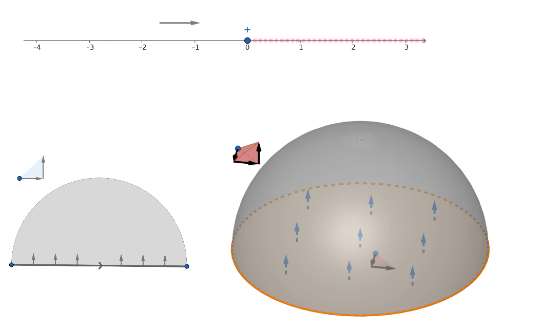
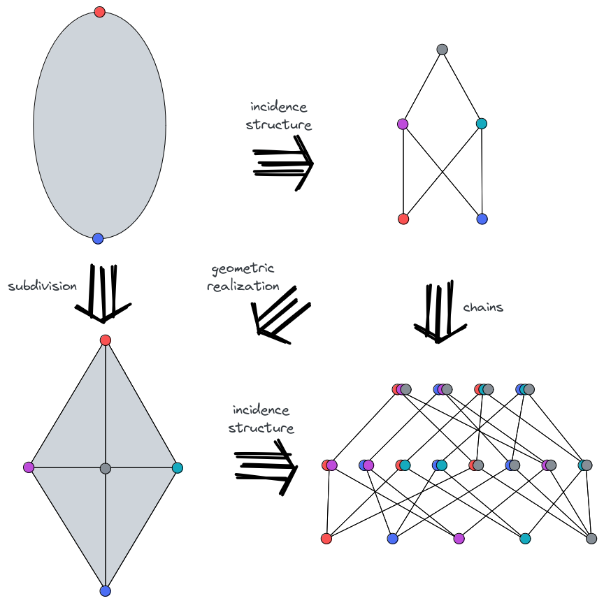
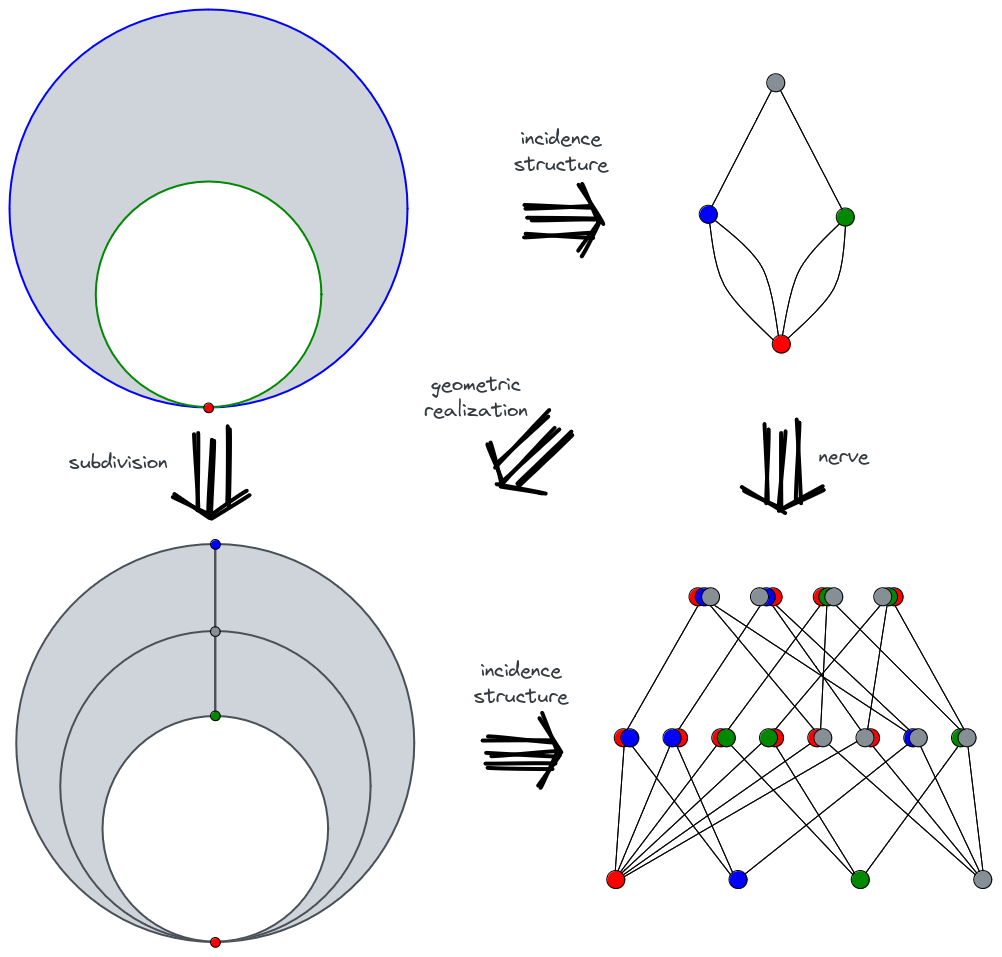
Under this constraint, the barycentric subdivision can be defined without geometric property. Recall that the barycentric subdivision of a conventional polytope is just the geometric realization (more precisely, the order complex) of its face lattice (see Figure 9). The barycentric subdivision of a semi-regular normal CW complex can be defined similarly, and it is just the geometric realization of the nerve of its incidence structure. In our definition of morphism chains, it should be defined as: the geometric realization of a nerve is constructed by making $(n{-}1)$-simplex for each non-degenerated $n$-chain $\langle\phi_{n},\dots,\phi_{2},\phi_{1}\rangle$ which is bounded by the corresponding simplexes of its direct subchains, where the orientation of this simplex should be defined such that the first boundary $\langle\phi_{n}\circ\phi_{n-1},\dots\rangle$ is positively-oriented with respect to it, and the second boundary $\langle\phi_{n},\phi_{n-1}\circ\phi_{n-2},\dots\rangle$ is negatively-oriented with respect to it, and so on. The $(-1)$-simplex is the null face. The geometric realization of the nerve of a semi-regular normal CW complex is just its barycentric subdivision (see Figure 10). More interestingly, the incidence structure of a vertex figure is just making a vertex figure of the geometric realization of upper closure of its incidence structure. There is a similar relation to the face figure. It shows “the incidence structure of a geometric object is related to the geometry of an incidence structure”. This series of articles will not discuss such correspondence further, since it only appears in a restricted incidence structure. In the next article, we will focus on finite bounded acyclic categories, and develop algorithms for them.

References

- [1] Anders Björner “Posets, regular CW complexes and Bruhat order” In European Journal of Combinatorics 5.1 Academic Press, 1984, pp. 7–16
- [2] Dimitry Kozlov “Combinatorial algebraic topology” Springer Science & Business Media, 2008
- [3] Peter McMullen and Egon Schulte “Abstract regular polytopes” Cambridge University Press, 2002