Accelerated Benders Decomposition and Local Branching for Dynamic Maximum Covering Location Problems
Abstract
The maximum covering location problem (MCLP) is a key problem in facility location, with many applications and variants. One such variant is the dynamic (or multi-period) MCLP, which considers the installation of facilities across multiple time periods. To the best of our knowledge, no exact solution method has been proposed to tackle large-scale instances of this problem. To that end, in this work, we expand upon the current state-of-the-art, branch-and-Benders-cut solution method in the static case, discussing several acceleration techniques. Additionally, we propose a specialised local branching scheme, which uses a novel distance metric in its definition of subproblems and features a new method for efficiently and exactly solving the subproblems. These methods are then compared with extensive computational experiments.
1 Introduction
A classic problem in operations research is the optimal location of facilities according to different aspects such as users’ preferences and installation cost. Within this category of problems is the maximum covering location problem (MCLP), attributed to Church and ReVelle (1974). In the MCLP, each facility covers the users within a certain radius and, due to limited resources, it is not possible to open every facility. Thus, a decision maker must select a subset of facilities to open, with the goal of maximising the total coverage. Due to its simplicity and versatility, the MCLP has been used in a wide range of applications, including emergency services location (Gendreau et al. 2001, Degel et al. 2015, Nelas and Dias 2020), healthcare services (Bagherinejad2018 and Shoeib 2018, Alizadeh et al. 2021), safety camera positioning (Dell’Olmo et al. 2014, Han et al. 2019), ecological monitoring or conservation (Church et al. 1996, Martín-Forés et al. 2021), bike sharing (Muren et al. 2020), and disaster relief (Zhang et al. 2017, Iloglu and Albert 2020, Yang et al. 2020). For a review of the MCLP and its applications, we refer to Murray (2016).
To include more complex interactions and restrictions, several variants of the MCLP have been developed. The one we consider is the dynamic (or multi-period) MCLP, where the decision maker conducts facility planning over a long time horizon, divided into discrete time periods (Schilling 1980, Gunawardane 1982). The intrinsic consideration of the time horizon is vital in many situations, such as when the demand to be covered varies across time (Porras et al. 2019), when planning infrastructure that will persist throughout future planning periods (Gunawardane 1982, Lamontagne et al. 2023), or in real-time operations of emergency services where exact positioning is important (Gendreau et al. 2001). Throughout the time horizon, open facilities may be forced to remain open for the duration of the time horizon (Lamontagne et al. 2023), may be allowed to change location with or without cost (Marín et al. 2018), or a subset may be required to relocated each time period (Dell’Olmo et al. 2014).
To the best of our knowledge, no exact method exists for solving large-scale dynamic MCLPs. More specifically, the only exact method employed in the literature for the dynamic MCLP is branch-and-bound, which has successfully solved instances with users, facilities, time periods (Dell’Olmo et al. 2014), and users, facilities, time periods (Lamontagne et al. 2023). Meanwhile, in terms of heuristic methods, Porras et al. (2019) used simulated annealing to solve instances with users, facilities, time periods, while Lamontagne et al. (2023) used a greedy method to solve instances with users, facilities, time periods. This compares with specialised methods for the static MCLP, which have successfully solved instances with users, facilities (Pereira et al. 2007), and users, facilities (Cordeau et al. 2019). Most notably, the method proposed in Cordeau et al. (2019) is specifically designed for problems in which there are significantly more users than facilities. This situation can occur when using a very fine discretisation of a continuous demand (e.g. Lamontagne et al. 2023) or when creating many different scenarios to model uncertainty in the problem (Daskin 1983, Berman et al. 2013, Vatsa and Jayaswal 2016, Nelas and Dias 2020). These categories of use cases support the need for a specialised method for the dynamic MCLP which can handle large-scale instances.
In this work, we present several contributions to the literature on the dynamic MCLP. First, we extend the branch-and-Benders-cut approach for the static MCLP of Cordeau et al. (2019) to the dynamic case. Second, we detail a suite of acceleration techniques tailored for the dynamic MCLP, which can be selected based on the structure of the application. This includes an intuitive and effective multi-cut generation technique, an efficient Pareto-optimal cut generation technique with a closed-form solution, a partial Benders decomposition strategy which leverages the problem structure, and a Benders dual decomposition approach which can further strengthen cuts for fractional solutions. Third, we present a specialized local branching method embedded within the branch-and-Benders cut framework. This method makes use of a new distance metric for defining subproblems, based on the problem structure. We then present a novel subproblem solution method, which can efficiently solve the local branching subproblems in an exact and proven-valid manner. Fourth, we present extensive computational results comparing our proposed methods. These experiments are carried out with instances based on real data from an electric vehicle charging station placement case study, underlying the practical interest of the dynamic MCLP. Our results validate the suitability of our methodological contributions to provide high-quality solutions to instances involving a large number of users, candidate locations and a planning horizon. In particular, our methods can produce solutions with a higher demand covered compared to the greedy heuristic in Lamontagne et al. (2023), in addition to providing performance guarantees via optimality gaps.
The rest of this paper is organized as follows: Section 2 discusses the literature about solution methods for the static and dynamic MCLP. Section 3 presents the general model for the dynamic MCLP. Section 4 is dedicated to the branch-and-Benders-cut methods, extending the work in Cordeau et al. (2019) and implementing improvement methods to the general framework. Section 5 then presents the local branching method, based on the work in Rei et al. (2009), with special consideration for the distance metric and the branching scheme. Finally, Section 6 provides our computational results, while Section 7 concludes our work.
2 Literature Review
Despite its long history, few exact solution methods have been developped for the MCLP, while heuristic methods are most commonly used (Murray 2016). We provide a summary of solution methods for both the static and dynamic MCLP in Table 1.
The most common exact method uses standard branch-and-bound techniques, in conjunction with off-the-shelf mixed-integer linear programming solvers. This method is commonly used for small-scale instances, or as a benchmark approach for heuristics. However, it has been repeatedly noted that this is insufficient for solving large-scale instances (see, e.g., ReVelle et al. 2008, Zarandi et al. 2013, Cordeau et al. 2019, Lamontagne et al. 2023). In addition, three other exact methods have been presented for the static MCLP. In Downs and Camm (1996), a lower bound is generated via a greedy procedure, similar to the one presented in Church and ReVelle (1974), while an upper bound is generated via Lagrangian relaxation of the covering constraints. Both are combined within a branch-and-bound framework to ensure optimality. In Pereira et al. (2007), the MCLP is reformulated as a p-median problem, with a column generation procedure used to solve the resulting model. In the procedure, stabilisation techniques are proposed to help improve the convergence rate, and limits are placed on both the number of columns generated and the total number of iterations. In Cordeau et al. (2019), the variables associated with the coverage of users are projected out in the Benders subproblem. An analytic solution is then given for the solution of the Benders dual subproblem, allowing for rapid generation of Benders cuts. This process is embedded within a branch-and-Benders-cut framework, allowing for large-scale problems to be solved efficiently.
In terms of heuristics, we note a wide variety of methods. However, two approaches which are used repeatedly include greedy methods and simulated annealing. In the greedy method (e.g. Church and ReVelle 1974), a solution is constructed by repeatedly opening a facility, each time selecting the one which causes the largest increase in coverage. In simulated annealing (e.g. Murray and Church 1996), the process simulates the cooling of metals, with a temperature parameter that varies across the solving process and which controls the mutability of our current solution (e.g. swapping an open facility for a closed one). In Xia et al. (2009), these two heuristics (along with greedy plus substitution, genetic algorithm and tabu search) were compared, with the simulated annealing method finding solutions of the best quality. By comparison, the greedy method solved instances faster, with solutions of value within a 1% relative gap of those of simulated annealing.
Our work contributes to the literature on exact methods for dynamic MCLPs, which, to our knowledge, is limited to branch-and-bound techniques. These have proved inadequate for tackling large-scale instances.
| Article | Variant | Methods proposed | Exact versus heuristic |
|---|---|---|---|
| Church and ReVelle (1974) | Static | Greedy, branch-and-bound | Both |
| Schilling (1980) | Dynamic | Weighing method | Heuristic |
| Gunawardane (1982) | Dynamic | Branch-and-bound | Exact |
| Downs and Camm (1996) | Static | Greedy + Lagrangian relaxation + Branch-and-bound | Exact |
| Galvão and ReVelle (1996) | Static | Greedy + Lagrangian relaxation | Heuristic |
| Murray and Church (1996) | Static | Greedy, simulated annealing | Heuristic |
| Adenso-Díaz and Rodríguez (1997) | Static | Tabu search | Heuristic |
| Resende (1998) | Static | GRASP | Heuristic |
| Galvão et al. (2000) | Static | Lagrangian relaxation, surrogate relaxation | Heuristic |
| Arakaki and Lorena (2001) | Static | Genetic algorithm | Heuristic |
| Gendreau et al. (2001) | Dynamic | Parallel tabu search | Heuristic |
| Pereira et al. (2007) | Static | Column generation | Exact |
| ReVelle et al. (2008) | Static | Heuristic concentration | Heuristic |
| Xia et al. (2009) | Static | Greedy, simulated annealing, genetic algorithm, tabu search | Heuristic |
| Rodriguez et al. (2012) | Static | Iterative greedy | Heuristic |
| Zarandi et al. (2013) | Dynamic | Simulated annealing | Heuristic |
| Dell’Olmo et al. (2014) | Dynamic | Branch-and-bound | Exact |
| Colombo et al. (2016) | Static | Variable neighbourhood search, heuristic concentration | Heuristic |
| Calderín et al. (2017) | Dynamic | Simulated annealing, evolutionary algorithm | Heuristic |
| Máximo et al. (2017) | Static | Intelligent-guided adaptive search | Heuristic |
| Marín et al. (2018) | Dynamic | Lagrangian relaxation | Heuristic |
| Cordeau et al. (2019) | Static | Branch-and-Benders-cut | Exact |
| Porras et al. (2019) | Dynamic | Simulated annealing | Heuristic |
| Lamontagne et al. (2023) | Dynamic | Greedy, GRASP, rolling horizon | Heuristic |
3 Problem Formulation
We present a general formulation for the dynamic MCLP. Let be the number of time periods, be the set of users and be the set of facilities. We use the index to denote a time period, the index for a user, and the index for a facility. We define the parameters such that if facility covers user in period , and otherwise. Let denote the demand of user in time period . We introduce a binary decision vector with entries such that if and only if facility exists in period . We also include in the model an auxiliary decision vector with entries such that if user is covered by some facility at period , and otherwise. Then, the dynamic maximum covering location is formulated as
| (1a) | |||||
| subject to | (1b) | ||||
| (1c) | |||||
| (1d) | |||||
| (1e) | |||||
The objective function (1a) maximises the demand covered over all time periods. Constraint (1b) defines the feasible domain for the variables , which can be any polytope not involving the variables . Typically, this includes either a cardinality constraint (e.g. Calderín et al. 2017) or a knapsack constraint (e.g. Cordeau et al. 2019) to restrict the number of facilities. The set can also include, for instance, diversification constraints imposing that the set of facilities must change in each time period (Dell’Olmo et al. 2014), or precedence constraints imposing that some facilities must be constructed before others (Lamontagne et al. 2023). Constraints (1c) impose that a suitable facility must exist for our users to be considered covered. Constraints (1d) and (1e) indicate that both sets of variables and must be binary. However, as noted in Murray (2016), integrality on the variables can be relaxed in Constraints (1e).
4 Benders Decomposition
In this section, we present an accelerated branch-and-Benders-cut approach tailored for the dynamic MCLP. This begins by generalising the current state-of-the-art approach in the static MCLP, the branch-and-Benders-cut method proposed by Cordeau et al. (2019), to the dynamic case. We then discuss acceleration techniques which aim to strengthen the formulation and accelerate convergence, applied within our dynamic context.
4.1 Single Cut Benders Decomposition
We detail the development of the branch-and-Benders-cut method proposed in Cordeau et al. (2019). While the process is nearly identical in the dynamic case as the static case, the development process is a prerequisite for the acceleration techniques we discuss below. As in Cordeau et al. (2019), we define as the set of users which are covered by only one facility.
Like in the classical Benders decomposition (Benders 1962), we project out the (continuous) variables of model (1). The value of the variables in the objective function is replaced with an auxiliary variable, . Then, in iteration , the main problem (MP) can be written as
| (3a) | |||||
| subject to | |||||
| (3b) | |||||
| (3c) | |||||
where and are the optimal dual vectors associated with the Benders subproblem in iteration . Since the Benders subproblem is feasible , it is not necessary to include feasibility cuts.
We denote —now and throughout this paper— as the candidate solution in iteration . Unless otherwise specified, it is assumed that this solution is integer feasible, i.e. that and . For each and , let denote the coverage of user in period by solution . When there is no risk of confusion, we use .
The Benders Primal Subproblem (BPS) is then given by
| (4a) | |||||
| subject to | (4b) | ||||
| (4c) | |||||
| (4d) | |||||
Let and denote the dual variables associated with Constraints (4b) and (4c). The Benders Dual Subproblem (BDS) is then
| (5a) | |||||
| subject to | (5b) | ||||
| (5c) | |||||
Similar to Cordeau et al. (2019), this subproblem can be easily solved by inspection: If , then the optimal solutions are . If , then . If , then any solution such that will be optimal. The optimality cut associated with these values is then
The resulting cut, reformulated as a function of the variables , is presented in Proposition 4.1. We set , and the left-hand side of the cut forms the term in (3b).
We remark that the names of the cuts (B0), (B1), and (B2) correspond to those of the equivalent cuts in Cordeau et al. (2019).
We note the following observations about these optimality cuts:
- •
-
•
By definition of the set , the condition will always be satisfied for .
- •
-
•
When evaluated at solution , the value of the left-hand side of the optimality cut (6) (and, thus, the corresponding objective value) matches the value of in Equation (2). This derives directly from the definition of . However, this evaluation is not correct (i.e. equal to in Equation (2)) in general if evaluated at a different solution.
We present a simple example of this in Figure 1. We drop the superscript as there is only one time period. If we generate the optimality cuts for the candidate solution , i.e. facility is opened whereas facilities and are closed, we have the following optimality cuts
(B0): (B1): (B2): All three types of cuts correctly identify the objective value of solution as , matching the value in Equation (2). However, if we then use these optimality cuts to calculate the objective value of the solution , we obtain the values and (for B0, B1, and B2 cuts respectively), while Equation (2) gives .
4.2 Improvements to the Single-Cut Method
In this section, we demonstrate and discuss the application of known techniques to our particular dynamic MCLP. These approaches aim to strengthen the Benders optimality cuts and improve the dual bound for the decomposition. For the sake of simplicity, the acceleration techniques are presented separately in relation to the decomposition presented in Section 4.1. However, it is possible to incorporate multiple techniques simultaneously. For a discussion of acceleration techniques in the general context of Benders decomposition, we refer to Rahmaniani et al. (2017).
There exist classes of improvement methods which heavily depend on the structure of , but which do not affect the structure of the Benders subproblems. Since they involve , their use is application-specific. However, since they do not impact the Benders subproblems, they can be applied to the methods in this work without affecting their validity. An example of such a technique would be a primal heuristic providing warmstart solutions. This can be used to obtain a good lower bound on the optimal objective value, which otherwise can be difficult during the early iterations of the Benders decomposition method (Rahmaniani et al. 2017). Another example would be valid cuts, which can be added to the main problem to tighten its linear programming (LP) relaxation. Examples for both techniques can be found in Santoso et al. (2005), Codato and Fischetti (2006), Costa et al. (2012).
The remainder of the techniques discussed in this section modify the Benders subproblems in some way, whether by changing the set of users (which, in turn, changes the amount of computational work required for the generation of cuts), modifying the frequency or type of cuts, or by directly providing reformulations for the BPS (4) or the BDS (5). When an aspect of the technique depends on the structure of (and thus may be application-specific), we include a discussion on this dependence.
Preprocessing
Preprocessing techniques which aggregate users reduce the size of and, consequently, the number of to be calculated in each iteration of the Benders decomposition. A method for doing this such that the resulting problem is equivalent is given in Legault and Frejinger (2022). Their method aggregates users based on their coverage from facilities, i.e., if users and are covered by exactly the same set of facilities then they can be aggregated. Heuristic methods also exist such as the ones by Dupačová et al. (2003) and Crainic et al. (2014). However, we note that, due to the analytic solution for the Benders dual subproblem, the marginal effects of each user is negligible in terms of the cut generation time.
Cut generation at fractional solutions
In Section 4.1, we observed that the Benders optimality cuts could be generated for both integer and fractional candidate solutions . In Cordeau et al. (2019), these cuts are generated at every node in the search tree, regardless if the corresponding solution is fractional or integer. However, in Botton et al. (2013), it was demonstrated that this can lead to an increase to the solving time, due to the computational effort required to generate the cuts with marginal benefits. As such, it was proposed to generate cuts at fractional solutions only at the root node.
Multi-cut method
Since the variables are only involved in the covering Constraints (1c), the Benders primal subproblem (4) can be separated per time period. This allows for more optimality cuts to be generated each iteration of the Benders decomposition, which accelerates convergence, as noted by Birge and Louveaux (1988) and Contreras et al. (2011). More specifically, we replace the auxiliary variable by the sum of new variables for . Then, for each iteration , we have the following MP:
| (7a) | |||||
| subject to | (7b) | ||||
| (7c) | |||||
| (7d) | |||||
where, as before, and are the optimal dual vectors associated with the Benders subproblem in time period and iteration . The BPS (4) and the BDS (5) as well as the process for deriving the Benders cuts is identical to the single-cut case, with the summations (and, as a consequence, indices) shifted from the subproblem to the main problem. The optimality cuts themselves are presented in Proposition 4.2.
While the Benders primal subproblem (4) can be separated per time period, it can also be separated by user. In fact, the preceding development can be done using auxiliary variables for and Benders primal subproblems defined for each time period and user. However, as this method is designed for large-scale instances with many users, such a decomposition may be computationally infeasible. Notably, while the multi-cut generation process given in Proposition 4.2 adds cuts in each iteration of the Benders decomposition, the equivalent version when separated by time period and by user would generated cuts in each iteration. As such, the number of constraints in the model would grow extremely rapidly each iteration of the Benders decomposition, quickly becoming intractable.
Pareto-optimal cuts
The optimal solution to the Benders dual subproblem may not be unique, and the strength of the resulting Benders cut may vary depending on the solution selected. This phenomenon is the principle behind the B0, B1, and B2-type cuts introduced in Proposition 4.1, with the strength of the resulting cuts discussed in depth in Cordeau et al. (2019). In the context of general Benders decomposition, the selection of an optimal solution leading to a Benders cut is introduced in Magnanti and Wong (1981). The authors propose a model for finding the strongest possible cut based on a core point, a point in the relative interior of the convex hull of . This technique was employed in Santoso et al. (2005), Contreras et al. (2011), and discussed further in Papadakos (2008).
Let be the candidate solution from the main problem (3) and be an associated optimal solution of the dual subproblem (5). Let denote a core point of . Magnanti and Wong (1981) define a Pareto-optimal cut with respect to a core point and a candidate solution as the one obtained by solving the following subproblem:
| (9a) | |||||
| subject to | (9b) | ||||
| (9c) | |||||
| (9d) | |||||
where is called a Pareto-optimal point.
Due to the presence of Constraint (9c), the Magnonti-Wong subproblem (9) is not quite identical to the Benders dual subproblem (5). Nevertheless, we are still able to describe the determination of an optimal solution to subproblem (9):
Proof.
We first emphasise that the solution to the Magnanti-Wong subproblem (9) must also be an optimal solution to the BDS (5) for , as specified in Magnanti and Wong (1981). This is enforced through Constraints (9b) and (9d) (which enforce feasibility), combined with Constraint (9c) (which enforces optimality). As described in Section 4.1, there is a set of optimal solutions to BDS (5) which can be analytically determined for each period and customer based on . Hence, let us denote by the set of optimal solution pairs . Concretely, recall that if , then . Likewise, implies that . Finally, if then .
In this way, we can equivalently formulate subproblem (9) with Constraint (9c) replaced by the following constraint:
This eliminates the linking constraint which involves all variables, reformulating the Magnonti-Wong subproblem (9) into the following:
| (10a) | ||||
| subject to | ||||
| (10b) | ||||
Now, it is easy to verify the feasibility and optimality of the solution described in the proposition statement. ∎
Corollary 4.1.
If the set is empty, then the Benders optimality cut is unique.
In practice, Proposition 4.2 states that, when determining if , we only need to consider the core point when . In those cases, rather than solely using information from and (as is the case for the cuts in Proposition 4.1), we can instead look to the coverage in the core point to determine if . If both and , then a different method is required. For example, it is possible to create analogous cuts to (B0), (B1), or (B2).
The calculation of Pareto-optimal points relies on finding a core point . Depending on the domain , it may not be possible to find a core point analytically. However, one may employ the iterative method proposed in Papadakos (2008), which starts with a feasible solution and takes the average with the candidate solution at every iteration to take the role of core point.
Benders Dual Decomposition
In Benders Dual Decomposition, information from the main problem is added to the Benders subproblems to generate better quality cuts. This is done via allowing some (or potentially all) of the upper level variables to change based on the dual information. Following the work in Rahmaniani et al. (2020), auxiliary variables are created by duplicating the decision variables . These auxiliary variables are then forced to match a fractional or integer candidate solution in the Benders subproblem, resulting in the following subproblem:
| (11a) | |||||
| subject to | (11b) | ||||
| (11c) | |||||
| (11d) | |||||
| (11e) | |||||
In its current form, the subproblem (11) is entirely equivalent to the original subproblem (4). However, by applying Lagrangian relaxation on the Constraints (11b), for a given Lagrangian multiplier for each and , we obtain the following Lagrangian subproblem:
| (12a) | ||||
| subject to | (12b) | |||
If we take as the optimal dual variables associated with Constraints (11b) after solving the subproblem (11) and as the optimal solutions of subproblem , this results in the optimality cuts
| (13) |
In Rahmaniani et al. (2020), it was shown that the cuts (13) are equivalent to the standard optimality cuts (6) when generated from an integer candidate solution . On the other hand, the authors also show that the cuts (13) are stronger than cuts (6) when generated from a fractional candidate solution.
If we further solve the full Lagrangian subproblem
| (14) |
with optimal solutions , we obtain the following optimality cuts:
| (15) |
As before, Rahmaniani et al. (2020) show that the cuts (15) are only useful for a fractional candidate solution, where the cuts (15) are stronger than both the standard optimality cuts (6) and the cuts (13).
However, in order to apply the Benders dual decomposition approach, we must repeatedly solve Lagrangian subproblems. Notably, depending on the structure of and the sizes of , solving the Lagrangian subproblems (12) or (14) may be computationally infeasible. As such, viability of this method is dependent on the application.
Partial Benders Decomposition
In Partial Benders Decomposition, information from the Benders subproblem is added to the main problem to improve the dual bound. This is done via including some variables of the Benders subproblem in the main problem. Following the work in Crainic et al. (2021), we partition into two sets, and , and define the following reformulation of the maximum covering problem:
| (16a) | |||||
| subject to | (16b) | ||||
| (16c) | |||||
| (16d) | |||||
| (16e) | |||||
| (16f) | |||||
This formulation is, clearly, equivalent to the original formulation (1). However, when we project the variables for the Benders decomposition, we keep the variables in the main problem. More specifically, in iteration of the Benders decomposition method, our main problem is given by
| (17a) | |||||
| subject to | (17b) | ||||
| (17c) | |||||
| (17d) | |||||
and the Benders primal subproblem is then given by
| (18a) | |||||
| subject to | (18b) | ||||
| (18c) | |||||
for which optimality cuts can be derived as before.
The users in are particularly well-suited for scenario retention, i.e. to make . If we take , by definition,, we have that . Next, we take the period and the facility such that . Then, since by definition, we have that Constraint (17c) will be satisfied with equality. As such, the variable can be removed from the main program (17), and the objective function can be replaced by
In addition to the scenario-retention method proposed in Crainic et al. (2021), the authors also propose a scenario-creation method. This involves the creation of artificial scenarios given by a convex combination of real scenarios. These artificial scenarios are then kept in the main problem as a proxy for their subproblem counterparts. However, this method relies on the variables , which are no longer present in the branch-and-Benders-cut framework presented in Section 4.1. As such, this approach is not suited for this framework.
5 Local Branching for Branch-And-Benders-Cut
In the local branching method by Fischetti and Lodi (2003) for tackling mixed-integer programs, small subdomains of the feasible space are defined via distance-based neighbourhoods around solutions. These small subdomains are then solved in a separate subproblem via a black-box solver, and excluded from the feasible space, thus gradually reducing the size of the search space. In Rei et al. (2009), this process was applied to a branch-and-Benders-cut framework, with the goal of simultaneously improving the upper and lower bounds for the search tree.
We start in Section 5.1 by presenting the framework (following the work in Rei et al. 2009) for embedding a local branching approach within our branch-and-Benders-cut method. This defines a modified main problem and the necessary subproblems, which are all reliant on a distance metric. In Section 5.2, we propose a new distance metric for the dynamic MCLP. Via this distance metric, we then provide a novel solution method for quickly solving subproblems. Finally, in Section 5.3, we discuss methods for separating the feasible subdomains explored in our subproblems.
5.1 Overview
We implement the local branching scheme within the framework of our branch-and-Benders-cut methods, as proposed in Rei et al. (2009). Since it is based on our branch-and-Benders-cut methods, any of the acceleration techniques presented in Section 4.2 can be applied to the local branching method as well. To that end, contrary to Section 4.2, we present this section using the multi-cut version of the Benders optimality cuts. Due to the central role of the time period in the proceeding developments, the multi-cut formulation allows for a more natural and interpretable explanation. Thus, at iteration of the Benders decomposition, we consider the following local branching main problem:
| (19a) | |||||
| subject to | |||||
| (19b) | |||||
| (19c) | |||||
where for are feasible facility location decisions previously determined. The function represents a distance metric, indicating that only solutions found at a distance from solution may be considered. We note that Constraints (19b) are the Benders optimality cuts (7c) provided by Proposition 4.2.
Our goal, given an integer candidate solution and a threshold distance , is to find the optimal solution to our original problem (1) restricted to distance around . As described in Rei et al. (2009), we can then generate Benders optimality cuts (8) for this high-quality solution, thus improving the upper bound in the local branching main problem (19). Simultaneously, the solution may also improve upon the incumbent, thus also increasing the lower bound. We can then exclude the subdomain of distance around from the local branching main problem (19) by adding a constraint of type (19c).
Formally, let denote the optimal solution to the restricted subproblem centered around , given by the solution to the following subproblem:
| (20a) | ||||
| subject to | ||||
| (20b) | ||||
If has a strictly higher objective than , we generate Benders optimality cuts (8) for , and we set and repeat the restricted problem (20) centered around . If , we create a diversified subproblem which replaces the threshold distance in Constraint (20b) with , and adds the constraint . This guarantees that the resulting optimal solution is different than , and we create Benders optimality cuts (8) from .
By setting , we ensure that the feasible domain in the restricted subproblem (20) in iteration and the main problem in iteration are complementary. More specifically, the restricted subproblem only considers solutions with distance , whereas the main problem considers solutions with distance . Since the candidate solution is integer feasible, it is not necessary to consider solutions with distance , as these correspond to fractional solutions.
We remark that the local branching main problem (19) and the restricted subproblem (20) can be defined via any distance metric and with any threshold distance . By increasing the size of the subdomain, we can remove a larger area from the feasible space of the local branching main problem (19), but at the cost of a restricted subproblem (20) that is harder to solve than that of a smaller size. We also note that any method can be used to find the optimal solution to the restricted subproblem (20). In Fischetti and Lodi (2003), a general-purpose mixed-integer linear solver is used, while the branch-and-Benders-cut approach with the acceleration techniques proposed in Section 4.2 is a natural choice in our case. However, by carefully selecting our distance metric and threshold distance , we can derive an exact solution method for the restriced subproblem (20) which is more effective than the accelerated branch-and-Benders-cut method.
5.2 An effective formulation for a tailored distance metric
The distance metric typically used is the Hamming distance (see, e.g., Fischetti and Lodi 2003, Rei et al. 2009). This results in Constraint (20b) taking the form
| (21) |
However, we propose to use a modified distance metric in the dynamic case, which enforces that the Hamming distance in each time period must be within our threshold. This results in Constraint (20b) taking the form
| (22) |
The motivation behind this new distance metric derives from infrastructure contexts, where the facilities under consideration correspond to significant investments (e.g. warehouses, stores, etc.). In those contexts, facilities which are added in early time periods are likely to persist throughout the time horizon. In the case of the general Hamming distance, this incurs a repeated penalty in each time period, increasing the total distance. As an illustration, consider the example in Figure 1 and the two solutions and , and a time horizon . These solutions are at distance when considering the general Hamming distance, whereas they are only at distance using the new metric.
An important benefit of this new distance metric allows for an efficient solving method if we consider . To describe this method we first note that, for a candidate solution and time period , there are only two sets of modifications which result in an integer solution at distance exactly :
-
1a)
Add one facility which is currently not selected.
-
1b)
Remove one facility which is currently selected.
Likewise, at distance exactly , there are only three sets of modifications:
-
2a)
Add two facilities which are currently not selected.
-
2b)
Remove one facility which is currently selected, and add one facility which is currently not selected.
-
2c)
Remove two facilities which are currently selected.
Since, by assumption and , options 1b) and 2c) cannot lead to an increase in the objective function, and hence, can be disregarded.
As a consequence, there is a limited number of feasible solutions contained within the restricted subproblem (20) when considering . We can then use Proposition 5.2 to evaluate the quality of feasible solutions (as given in Equation (2)) based on Benders optimality cuts.
Proof.
We first note that, by rearranging the terms in the left-hand side, we have that
Now, we concentrate on both cases for .
If is given by (B0), then we have that
where implies that , since all elements in the summation are binary.
From there, for the first term, being binary also implies that . As such, we have that
. For the second term, we note that since has an extra facility compared to , we also have that the coverage for each user must be equal or greater. Concretely, , and thus .
As a consequence, we have that
If is given by (B1), then we have that
We note that, by definition of the set , we always have that . As a consequence, we have that . The last two terms can be transformed using reasoning similar to that of the prior case, which gives our result.
∎
We remark that Proposition 5.2 does not hold in general if is given by (B2). As a counterexample if is given by (B2), consider the example illustrated in Figure 1, the candidate solution , and . We then have that and .
Put more simply, Proposition 5.2 states that if we take a given solution and only add one facility to it, then the Benders optimality cuts for accurately give the coverage for the modified solution.
We can then derive an efficient method for finding the optimal solution of distance two around by combining the limited number of valid modifications to along with Proposition 5.2. For this, let denote the elemental vector with in position and elsewhere. We then denote (respectively, ) as the modified solution which adds the currently unused facility in period (respectively, removes the currently used facility ). We present this method in Proposition (5.2).
Proof.
The feasible space for the variables are defined via Constraints (1b), (1d), (19c), and (23b). Since these constraints are present in both models, it follows that the set of feasible values for are the same. We now show that the objective value for every feasible solution is the same in both models.
From our previous discussion, there is a limited number of feasible solutions which we must consider: the solution itself, as well as the resulting solutions from modifications 1a), 2a) and 2b). The value of the solution is given by Constraint (23c). For all other solutions, we make use of Proposition 5.2. More specifically, for each type of modification, we have generated an optimality cut for a solution with exactly one fewer facilities:
- •
- •
- •
∎
We note the following observations about Proposition 5.2:
-
•
Due to the presence of Constraints (1d), model (23) is a mixed-integer linear program, which can be solved directly via a generic MILP solver. When solving model (23) directly with a generic solver is the strategy for finding the optimal solution to the restricted subproblem (20), we denote this as SubD . When, instead, the restricted subproblem (20) is solved via the branch-and-Benders-cut method, we denote this SubB .
-
•
Some of Constraints (23c)-(23e) may be redundant, in the sense that they allow for the evaluation of solutions which can either be evaluated using other constraints within the model or which correspond to infeasible solutions. In general, verifying the feasibility of the solutions before generating the associated Constraints (23d) or (23e) is unlikely to be beneficial, due to the speed at which these constraints can be built. Instead, infeasible solutions can be detected by the MILP solver via Constraints (1b) and (19c). However, some structures of may make the detection of some infeasible solutions a trivial task, such as the use of precedence constraints, and thus justify the computational effort of the verification process.
-
•
From the proof of Proposition 5.2, it is clear that the optimal objective value of the restricted subproblem (20) and of model (23) are the same. This is important, as it allows us to verify if the newly found solution has a better objective value than the incumbent, and update the incumbent accordingly.
5.3 Branching
Using Proposition 5.2, we can thus easily solve the restricted subproblem (20). However, this ease of solving comes at a cost when moving to solve the full problem (19).
After each candidate solution and the set of restricted and diversified subproblems, the Constraints (19c) ensure that the solver removes the subdomain examined during the subproblems, thus avoiding unnecessary work. In Rei et al. (2009), the Hamming distance is used in Constraints (19c), and hence, the complement of the set is simply
However, using the distance metric in Section 5.2, the set requires the Hamming distance to be at least in at least one time period, which cannot be modeled as a single linear constraint. Therefore, we must create a branch for each time period in order to mimic through disjoint problems. More specifically, for every , we generate the following problem:
| (24a) | ||||
| subject to | ||||
| (24b) | ||||
| (24c) | ||||
Each of these problems can be viewed as a branch at node in the search tree. In this way, the Constraints (19c) are formed of the branching constraints (24b) and (24c) from the prior nodes in the search tree. In essence, these branches progressively select each time period as the one that exceeds the threshold distance, and impose all prior years to be below the threshold in order to ensure distinct sets. When using these branches to separate the subdomains of the restricted and diversified subproblems, we refer to the method as SepB .
Alternatively, we can model this disjunction through a set of cuts, requiring the introduction of auxiliary binary variables and Big-M constraints. More specifically, the set can be obtained by adding to Constraints (19c) the constraints
| (25a) | |||||
| (25b) | |||||
| (25c) | |||||
However, since we are adding the binary variables and the Big-M constraints (25a) to the main program (19), the problem gets progressively more difficult to solve as more subdomains are removed.
We note that in the case that the distance , the Constraints (25) are equivalent to (and thus can be replaced by) the typical no-good cut:
| (26) |
which does not require the use of binary auxiliary variables.
6 Computational experiments
In this section, we compare the performance of the variations of the Benders decomposition techniques presented in this work. We start in Section 6.1 by giving the background information for the problem instances, which are obtained from an electric vehicle (EV) charging station location model, and based on real-life data. In Section 6.2, we then examine the performance metrics when using our Benders decomposition methods to solve these problem instances, which clearly demonstrates the capabilities and limitations of each method on a practical example. In Section 6.3, we evaluate the options for the local branching method presented in Section 5.2 for the restricted subproblem solution method. These experiments demonstrate the efficiency of solving our reformulated restricted subproblem (23), validating its use in Section 6.2. Similarly, in Section 6.4, we compare the options for eliminating feasible space already explored within the local branching method, as presented in Section 5.3. Additionally, we discuss the technical limitations that face the implementation of the SepB method, and the consequences of using either the SepD or SepB methods.
To more easily distinguish between the methodologies discussed in this paper, we present the following nomenclature:
-
1.
The unaccelerated branch-and-Benders-cut procedure in Cordeau et al. (2019) as described in Section 4.1 is referred to as the U-B&BC method. This procedure is unaccelerated in the sense that it does not include any of the acceleration techniques presented in Section 4.2. In particular, this method generates Benders optimality cuts (6) at every integer and fractional candidate solution.
-
2.
The accelerated branch-and-Benders-cut procedure presented in Section 4.2 is referred to as the A-B&BC method. As some techniques are dependent on the instance characteristics, we describe the set of acceleration techniques in more detail in Section 6.1. Notably, for the A-B&BC method, Benders optimality cuts are generated for every integer candidate solution, while Benders optimality cuts are generated for fractional candidate solutions only at the root node.
-
3.
The accelerated branch-and-Benders-cut procedure with local branching presented in Section 5 is referred to as the A-B&BC+LB-Sub-Sep method, where Sub indicates the restricted subproblem solution method as described in Section 5.2 and Sep indicates the subdomain separation scheme as described in Section 5.3. In all cases, we impose a time limit of 60 seconds for the solving of each restricted and diversified subproblem, after which the the best incumbent solution is used for the subsequent procedures.
Regardless of the subproblem solution method and the subdomain separation scheme, almost all acceleration techniques are identical between the A-B&BC and A-B&BC+LB-Sub-Seb methods. The one exception is the generation of optimality cuts for fractional solutions. It was observed that, in the hard instances, both the U-B&BC and A-B&BC methods spent a considerable amount of time in the root node generating optimality cuts for fractional solutions. Since the SepB separation scheme relies on branching, we push the solver to exit the root node more quickly. To do this, we solve the continuous relaxation of the model using the multi-cut method, then keep the resulting (fractional) optimality cuts in the formulation. We then solve the MILP formulation of the problem and only generate optimality cuts for integer solutions. This procedure is similar to the one proposed in Fortz and Poss (2009), where feasibility cuts for fractional solutions are only generated as part of solving the LP relaxation.
The tests were run on a server running Linux version 3.10, with an Intel Core i7-4790 CPU with eight virtual cores and 32 GB of RAM. The code is written in C++, and is publicly available111https://github.com/StevenLamontagne/BendersDecomposition. We use CPLEX version 22.1.1 limited to a single thread, and with the Benders cuts implemented via the generic callback feature. Other than the removal of incompatible preprocessing and reformulation options in the cases which use the callback feature, the only notable parameters which are not set at default value are the memory management and numerical precision. The Eigen library (Guennebaud et al. 2010) is used for efficient dense and sparse matrix calculations, notably for the calculation of and the subsequent generation of cuts. In all tests, we impose a two-hour (7,200 second) time limit for solving each instance.
6.1 Application: Electric vehicle charging station placement
We apply the proposed methods to the instances of the electric vehicle (EV) charging station placement problem by Lamontagne et al. (2023). We chose these problem instances because of their practical interest and the large number of users, which leads to large-scale dynamic MCLPs and therefore allows us to demonstrate the capabilities of our methodological contributions.
In this problem, there are two groups making sequential decisions over a multi-period time span. First, a decision maker which decides where to place public charging infrastructure. And second, users purchasing a vehicle in the given time period, who must elect between an EV or a conventional vehicle (a choice which depends on the charging network). If a user is covered by a charging station (in the maximum covering sense), then they elect to purchase an EV. The objective of the decision maker is to place the charging infrastructure in such a way as to maximise EV adoption.
In addition to determining which charging stations to open, this problem also aims to find the optimal sizing (i.e. number of charging outlets) of each open station. For this purpose, the decision variables are binary, indicating if a charging station has at least outlets (with ranging from to an upper bound ). The set is then composed of three sets of constraints: precedence constraints imposing for each station that in order to have at least outlets, one must first have at least outlets, constraints that forbid the removal of outlets between time periods, and budget constraints which force the cost of installing new outlets to be below a budget in each time period.
The test instances are divided into five datasets, each with different characteristics and each containing 20 instances. We refer to Lamontagne et al. (2023) for a detailed description. However we note that the Simple, Distance, and HomeCharging datasets are easier to solve than the LongSpan and Price datasets. Notably, no instances in the latter two datasets were solved exactly in Lamontagne et al. (2023), with the best incumbent objective value in the branch-and-cut method (via CPLEX 12.10) being below that of the greedy method described in that paper. As a consequence, we refer to the set of instances in the Simple, Distance, and HomeCharging datasets as the “easy instances”, while those from the LongSpan and Price datasets are called the “hard instances”.
Next, we discuss the customisation of the acceleration techniques described in Section 4.2 used for this problem.
-
•
There are two preprocessing techniques we can use to eliminate users from consideration, without affecting the objective value. The first technique, as proposed in Legault and Frejinger (2022), is to eliminate any users for which . Note that such users they can never be covered regardless of our efforts, implying that their elimination does not affect the objective. The second technique is to eliminate any user which is “precovered” (in the sense that there is an existing facility or option which guarantees coverage, regardless of decisions in the model). In particular, in the HomeCharging dataset, there are users who have access to a home charging system for their EV. As a consequence, a subset of those users will purchase an EV, regardless of the state of the public charging network, and can be eliminated from consideration.
-
•
For a heuristic warmstart, we use the greedy method proposed in Lamontagne et al. (2023). This is achieved via the warmstart feature present in CPLEX.
-
•
We keep the users within the main problem, as described in Section 4.2.
-
•
For the Benders optimality cuts, we use the multicut equivalent of the Pareto-optimal cuts in Proposition 4.2, using B1-type cuts. In other words, for , the sets in Proposition 4.2 are given by
(27) The users do not need to be considered, due to the partial Benders decomposition strategy mentioned above. We use the iterative method proposed in Papadakos (2008) for estimating a core point.
-
•
In the cases of the LongSpan and Price datasets, CPLEX is unable to solve even the linear programming relaxation of model (1) as shown in Lamontagne et al. (2023). As such, we do not use Benders dual decomposition, as repeatedly solving the Lagrangian subproblems (12) or (14) would be computationally infeasible.
6.2 Comparison of methodologies
In this section, we compare the performance of the U-B&BC , A-B&BC , and A-B&BC+LB-SubD-SepD methods for solving the instances. As will be discussed later, these options for the local branching method are the best suited for our application. Additionally, we compare these with a standard branch-and-cut tree via CPLEX, and the greedy method from Lamontagne et al. (2023). These last two methods are referred to as the B&C and Greedy methods, respectively. We note that the A-B&BC and A-B&BC+LB-SubD-SepD methods both use the Greedy method as a warmstart, and thus will always terminate with an objective value that is at least equal to it.
In Table 2, we summarise our computational results for each methodology and instance set. The solving time, objective value, optimality gap, and number of nodes are reported as given by CPLEX. However, we note that the number of nodes in the local branching case only includes the ones for the main problem. By examining the results, we note that:
-
•
While the U-B&BC method is able to find a non-trivial solution (i.e. a solution which places at least one facility) for all instances, it found worse quality solutions on average than the Greedy method, A-B&BC , and A-B&BC+LB-SubD-SepD methods in the hard instances.
-
•
The A-B&BC method was able to outperform the U-B&BC method in all instances. In addition, in the easy instances, the A-B&BC method is able to run faster than the B&C method. However, while it is able to reduce the optimality gap in the hard instances compared to the U-B&BC method, the objective value is only slightly better than the Greedy method. In fact, the A-B&BC method only improved the objective value compared to the Greedy method in two instances in the LongSpan dataset, and two instances in the Price dataset.
-
•
The A-B&BC+LB-SubD-SepD method required more time than either the A-B&BC or the B&C methods in the easy instances, and the optimality gap is considerably higher than the A-B&BC method in the hard instances. However, the A-B&BC+LB-SubD-SepD method improves the objective value compared to the Greedy method in all 20 instances in the LongSpan dataset and 17 instances in the Price dataset, which is notably more than the A-B&BC method.
Additional performance details are presented in A.1.
| Simple | Distance | HomeCharging | LongSpan | Price | ||
| Solve time (sec) | Greedy | 0.05 | 0.10 | |||
| B&C | 0.20 | 0.70 | 6.56 | 7186.12 | 7194.97 | |
| U-B&BC | 0.15 | 1.57 | 68.24 | 7184.25 | 7184.76 | |
| A-B&BC | 0.09 | 0.52 | 1.34 | 7184.54 | 7185.04 | |
| A-B&BC+LB-SubD-SepD | 4.67 | 4.81 | 13.00 | 7291.34 | 7305.71 | |
| Objective value | Greedy | 31814.20 | 16591.75 | 18016.47 | 133724.37 | 33641.74 |
| B&C | 31820.15 | 16627.14 | 18030.50 | 0.00 | 0.00 | |
| U-B&BC | 31820.15 | 16627.14 | 18030.47 | 116663.50 | 32563.31 | |
| A-B&BC | 31820.15 | 16627.14 | 18030.40 | 133728.65 | 33642.19 | |
| A-B&BC+LB-SubD-SepD | 31820.15 | 16627.14 | 18030.49 | 133781.88 | 33650.81 | |
| Optimality gap (%) | B&C | - | - | |||
| U-B&BC | 15.79 | 15.00 | ||||
| A-B&BC | 6.12 | 11.32 | ||||
| A-B&BC+LB-SubD-SepD | 11.86 | 18.66 | ||||
| Number of nodes | B&C | 59.25 | 43.35 | 131.95 | 0.00 | 0.00 |
| U-B&BC | 52.40 | 27.85 | 228.50 | 0.00 | 0.00 | |
| A-B&BC | 65.35 | 75.05 | 860.45 | 0.00 | 1499.60 | |
| A-B&BC+LB-SubD-SepD | 65.05 | 205.60 | 797.35 | 7282.65 | 1202.50 |
6.3 Further results: Local branching restricted subproblem solution method
In this section, we compare the methods for solving the restricted subproblems (20) of the local branching procedure. Since these subproblems are solved many times in each instance, it is imperative that they are solved efficiently. For this, we use the SubD and SubB procedures presented in Section 5.2. We recall that the SubD method solves the restricted subproblem (20) by directly providing the reformulation (23) to a generic MILP solver (in this case, CPLEX), while the SubB procedure solves the restricted subproblem (20) with the A-B&BC method.
For a more accurate comparison between the SubD and SubB methods, we simulate the entire solving process. This starts with the MP (19), with no optimality cuts (7c) nor feasible space reductions (19c). We then generate randomly a sequence of 255 feasible candidate solutions , which are used for both SubD and SubB methods. For each solution, we solve the resulting restricted problem (20) using each method. Then, we add the Constraints (25) and the Benders optimality cuts derived from the set (27) for , and continue to the next solution.
In Table 3, we report the average results across all instances in each dataset. The objective value and solve times are as reported as CPLEX, however only instances which terminate before the time limit are included in the solve time. For the subproblems solved it is indicated the percentage of the subproblems which were successfully solved before the time limit was reached.
Examining the results, we note that both methods performed nearly identically in the easy instances. Additionally, in terms of solving time, both methods were very similar in the hard instances. By contrast, the percentage of subproblems solved within the time limit is drastically different between the two methods, with the SubD method successfully solving nearly all instances whilst the SubB method is able to solve very few. This can also be seen in the objective values, with the average objective value for the SubD method being better than the SubB method in the hard instances. These results demonstrate quite clearly that the proposed method is much better for solving the subproblem in hard problems compared to the SubB method.
A detailed view of the evolution of the solve times in terms of the number of evaluated solutions is presented in Appendix A.2. In brief, we observe a similar increase in the solve time for both methods, with more variability in the SubB method.
| Simple | Distance | HomeCharging | LongSpan | Price | ||
|---|---|---|---|---|---|---|
| Objective value | SubD | 25382.61 | 12539.70 | 15817.63 | 130526.42 | 32559.12 |
| SubB | 25382.61 | 12539.70 | 15817.63 | 130462.23 | 32544.02 | |
| Solve time (fully solved, sec) | SubD | 0.07 | 0.16 | 0.21 | 30.78 | 14.67 |
| SubB | 0.08 | 0.14 | 0.20 | 38.84 | 14.39 | |
| Subproblems solved (%) | SubD | 100.00 | 100.00 | 100.00 | 89.04 | 100.00 |
| SubB | 100.00 | 100.00 | 100.00 | 1.75 | 5.69 |
6.4 Further results: Local branching subdomain separation scheme
In this section, we compare the two distinct approaches presented in Section 5.3 for exploring the disjoint search spaces in the local branching subproblems. We recall that the SepB approach consists in creating a series of branches indicating the time period for which the distance from our candidate exceeds the distance threshold. These branches can be created after any feasible solution, and so we compare branching after every iteration of the Benders decomposition with branching only in iterations of the Benders decomposition for which the solution found is better than the current incumbent. The SepD approach consists in using the Constraints (25) to model the disjunctive set. These constraints are added for every candidate solution encountered during the series of restricted and diversified subproblems.
From technical standpoint, it is only possible to create two branches at every branch-and-bound node of CPLEX (IBM 2022). As the SepB approach demands a branch per time period, this comparison is only possible for . Since all of the problem instances contain at least four time periods, we modify the instances in this section by not considering any time periods beyond the first two.
In Table 4, we see the average results across all instances in each dataset. The solve time, objective value, and optimality gap are reported directly by CPLEX. The number of diversified subproblems and restricted subproblems are collected as part of the callback, and include all subproblems regardless of their solution status. The number of local branching separations is also collected as part of the callback, and reports the number of branches created as part of the separation procedure.
By examining the results, we observe that the SepB method which branches after every iteration had the worst performance overall. In particular, the objective value is lower and the optimality gap is higher than both other methods. Comparing the SepD and the SepB method which branches only after improving solutions, we see a trade-off in terms of objective value and optimality gap. There is also a notable difference in terms of the number of restricted subproblems, with the SepD method performing roughly 50% more subproblems.
To better explain this difference, it is important to keep in mind how both the SepB and SepD methods work at a high level. On the one hand, the SepB method creates two branches at the candidate solution, corresponding to the threshold distance being exceeded in either the first time period or the second. As such, each of these branches solves the main problem (19) at a local level, within relatively large subdomains. By selecting to explore a subdomain which contains better quality solutions, the solver can then improve the incumbent. However, as the subdomains get more restrictive, the bounds provided by the Benders optimality cuts become more accurate, making it more difficult to find new, improving nodes to explore. Additionally, as a consequence of this branching procedure, any upper bounds that are found are locally valid, leading to a decreased optimality gap in unexplored branches. On the other hand, the SepD method effectively creates a hole within the feasible domain, imposing that all solutions must exceed the threshold distance. As such, the main problem (19) is working at a global level, not divided into subdomains. This may make it easier to find new, improving nodes, as the solver may easily move to areas of the feasible domain which have not been explored and, thus, areas in which the bounds from the Benders optimality cuts are less accurate. Additionally, since the main problem works at a global level, any upper bounds that are found are globally valid, leading to an improved optimality gap overall. Due to the black-box nature of the solver, it is not possible to verify this hypothesis. However, it is supported by the progressively increasing number of nodes and the progressively decreasing optimality gap from the SepB method at all solutions, to the SepB method at improving solutions, and then to the SepD method.
These results suggest that it may be beneficial to consider the SepB method for subproblem separation at improving solutions when higher-quality feasible solutions are sought. However, the limitations in terms of the number of time periods would need to be addressed in order to apply the SepB method more generally.
Additional performance details are presented in A.3.
| Simple | Distance | HomeCharging | LongSpan | Price | ||
|---|---|---|---|---|---|---|
| Solve time (sec) | SepB , all solutions | 46.52 | 2.32 | 1460.34 | 7176.68 | 9045.39 |
| SepB , improving solutions | 0.72 | 1.17 | 8.95 | 7192.53 | 7269.47 | |
| SepD | 1.12 | 1.68 | 4.99 | 7175.38 | 7292.31 | |
| Objective value | SepB , all solutions | 13718.14 | 6635.17 | 8151.72 | 18473.34 | 13439.35 |
| SepB , improving solutions | 13718.14 | 6634.57 | 8151.48 | 18882.63 | 13601.62 | |
| SepD | 13718.14 | 6634.37 | 8151.48 | 18851.94 | 13552.85 | |
| Optimality gap (%) | SepB , all solutions | 0.21 | 21.92 | 22.41 | ||
| SepB , improving solutions | 13.38 | 18.05 | ||||
| SepD | 12.47 | 17.47 | ||||
| Number of nodes | SepB , all solutions | 509.10 | 100.60 | 3061.90 | 1003.45 | 589.73 |
| SepB , improving solutions | 12.75 | 73.95 | 216.35 | 2654.30 | 1117.95 | |
| SepD | 10.00 | 64.10 | 170.80 | 4273.90 | 1592.75 | |
| Number of diversified subproblems | SepB , all solutions | 662.45 | 26.70 | 2892.20 | 760.50 | 278.27 |
| SepB , improving solutions | 13.60 | 13.05 | 61.80 | 889.15 | 276.30 | |
| SepD | 18.00 | 15.85 | 30.55 | 876.80 | 268.90 | |
| Number of restricted subproblems | SepB , all solutions | 1424.90 | 98.25 | 13127.65 | 4838.15 | 1708.62 |
| SepB , improving solutions | 31.25 | 41.60 | 195.60 | 4783.15 | 1338.45 | |
| SepD | 87.75 | 101.95 | 170.40 | 6773.35 | 1973.20 | |
| Number of user-created branches | SepB , all solutions | 654.70 | 27.00 | 2887.90 | 741.20 | 260.38 |
| SepB , improving solutions | 2.20 | 4.70 | 6.70 | 12.40 | 9.30 |
7 Conclusion
In this work, we present two new methods for solving the dynamic MCLP in an exact manner. The accelerated branch-and-Benders-cut method expands upon the current state-of-the-art in the static case, the Benders decomposition in Cordeau et al. (2019), adding several acceleration techniques from the literature to improve convergence. Computational experiments showed that the proposed method resulted in better performance across solving time, objective value, and optimality gap compared to the state-of-the-art. Additionally, the general nature of the model and the acceleration techniques may allow for the improved method to be applied to different structures of . For example, the dynamic equivalent to the budgeted MCLP (Khuller et al. 1999, Li et al. 2021, Wei and Hao 2023) or the MCLP under uncertainty (Daskin 1983, Berman et al. 2013, Vatsa and Jayaswal 2016, Nelas and Dias 2020).
The accelerated branch-and-Benders-cut method with local branching develops a specialised local branching scheme for the dynamic MCLP. This combines an intuitive distance metric with an innovative subproblem solution method to find improved feasible solutions. Indeed, in computational experiments, this method was the only one able to consistently find better quality feasible solutions compared to the warmstart solution.
Both methods were applied to an existing problem in the literature, an EV charging station placement model (Lamontagne et al. 2023). This provided faster solution methods with better performance guarantees, as well as improved lower bounds. These results validate the methodological contributions provided in this work for the dynamic MCLP.
From our experiments, we conclude that potential speedups should exploit the structure of . In other words, it is crucial to obtain primal formulations in which the linear relaxation is tight in the main problem variables. Hence, future work on specific dynamic MCLPs could follow this research direction in order to improve the performance of our Benders framework.
Acknowledgements
The authors gratefully acknowledge the assistance of Jean-Luc Dupré from Direction Mobilité of Hydro-Québec for sharing his expertise on EV charging stations and the network, as well as Ismail Sevim for his insights into the project. We also gratefully acknowledge the assistance of Walter Rei of Université de Québec à Montréal and Mathieu Tanneau of Georgia Institute of Technology in discussion about Benders decomposition techniques.
This research was supported by Hydro-Québec, NSERC Collaborative Research and Development Grant CRDPJ 536757 - 19, and the FRQ-IVADO Research Chair in Data Science for Combinatorial Game Theory.
References
- Adenso-Díaz and Rodríguez (1997) B. Adenso-Díaz and F. Rodríguez. A simple search heuristic for the MCLP: Application to the location of ambulance bases in a rural region. Omega, 25(2):181–187, 1997.
- Alizadeh et al. (2021) Roghayyeh Alizadeh, Tatsushi Nishi, Jafar Bagherinejad, and Mahdi Bashiri. Multi-period maximal covering location problem with capacitated facilities and modules for natural disaster relief services. Applied Sciences, 11(1), 2021.
- Arakaki and Lorena (2001) Reinaldo Gen Ichiro Arakaki and Luiz Antonio Nogueira Lorena. A constructive genetic algorithm for the maximal covering location problem. In Proceedings of metaheuristics international conference, pages 13–17, 2001.
- Bagherinejad2018 and Shoeib (2018) Jafar Bagherinejad2018 and Mahnaz Shoeib. Dynamic capacitated maximal covering location problem by considering dynamic capacity. International Journal of Industrial Engineering Computations, 9(2):249–264, 2018.
- Benders (1962) Jacques F. Benders. Partitioning procedures for solving mixed-variables programming problems. Numerische mathematik, 4(1):238–252, 1962.
- Berman et al. (2013) Oded Berman, Iman Hajizadeh, and Dmitry Krass. The maximum covering problem with travel time uncertainty. IIE Transactions, 45(1):81–96, 2013.
- Birge and Louveaux (1988) John R. Birge and François V. Louveaux. A multicut algorithm for two-stage stochastic linear programs. European Journal of Operational Research, 34(3):384–392, 1988.
- Botton et al. (2013) Quentin Botton, Bernard Fortz, Luis Gouveia, and Michael Poss. Benders decomposition for the hop-constrained survivable network design problem. INFORMS Journal on Computing, 25(1):13–26, 2013.
- Calderín et al. (2017) Jenny Fajardo Calderín, Antonio D. Masegosa, and David A. Pelta. An algorithm portfolio for the dynamic maximal covering location problem. Memetic Computing, 9(2):141–151, 2017.
- Church and ReVelle (1974) Richard Church and Charles ReVelle. The maximal covering location problem. In Papers of the regional science association, volume 32, pages 101–118. Springer-Verlag Berlin/Heidelberg, 1974.
- Church et al. (1996) Richard L. Church, David M. Stoms, and Frank W. Davis. Reserve selection as a maximal covering location problem. Biological Conservation, 76(2):105–112, 1996.
- Codato and Fischetti (2006) Gianni Codato and Matteo Fischetti. Combinatorial Benders’ cuts for mixed-integer linear programming. Operations Research, 54(4):756–766, 2006.
- Colombo et al. (2016) Fabio Colombo, Roberto Cordone, and Guglielmo Lulli. The multimode covering location problem. Computers & Operations Research, 67:25–33, 2016.
- Contreras et al. (2011) Ivan Contreras, Jean-François Cordeau, and Gilbert Laporte. Benders decomposition for large-scale uncapacitated hub location. Operations Research, 59(6):1477–1490, 2011.
- Cordeau et al. (2019) Jean-François Cordeau, Fabio Furini, and Ivana Ljubić. Benders decomposition for very large scale partial set covering and maximal covering location problems. European Journal of Operational Research, 275(3):882–896, 2019.
- Costa et al. (2012) Alysson M. Costa et al. Accelerating Benders decomposition with heuristic master problem solutions. Pesquisa Operacional, 32(1):3–19, 2012.
- Crainic et al. (2014) Teodor Gabriel Crainic, Mike Hewitt, and Walter Rei. Scenario grouping in a progressive hedging-based meta-heuristic for stochastic network design. Computers & Operations Research, 43:90–99, 2014.
- Crainic et al. (2021) Teodor Gabriel Crainic, Mike Hewitt, Francesca Maggioni, and Walter Rei. Partial Benders decomposition: General methodology and application to stochastic network design. Transportation Science, 55(2):414–435, 2021.
- Daskin (1983) Mark S. Daskin. A maximum expected covering location model: Formulation, properties and heuristic solution. Transportation Science, 17(1):48–70, 1983.
- Degel et al. (2015) Dirk Degel, Lara Wiesche, Sebastian Rachuba, and Brigitte Werners. Time-dependent ambulance allocation considering data-driven empirically required coverage. Health Care Management Science, 18(4):444–458, 2015.
- Dell’Olmo et al. (2014) Paolo Dell’Olmo, Nicoletta Ricciardi, and Antonino Sgalambro. A multiperiod maximal covering location model for the optimal location of intersection safety cameras on an urban traffic network. Procedia - Social and Behavioral Sciences, 108:106–117, 2014.
- Downs and Camm (1996) Brian T. Downs and Jeffrey D. Camm. An exact algorithm for the maximal covering problem. Naval Research Logistics (NRL), 43(3):435–461, 1996.
- Dupačová et al. (2003) J. Dupačová, N. Gröwe-Kuska, and W. Römisch. Scenario reduction in stochastic programming. Mathematical Programming, 95(3):493–511, 2003.
- Fischetti and Lodi (2003) Matteo Fischetti and Andrea Lodi. Local branching. Mathematical Programming, 98(1):23–47, 2003.
- Fortz and Poss (2009) B. Fortz and M. Poss. An improved Benders decomposition applied to a multi-layer network design problem. Operations Research Letters, 37(5):359–364, 2009.
- Galvão et al. (2000) Roberto D. Galvão, Luis Gonzalo Acosta Espejo, and Brian Boffey. A comparison of Lagrangean and surrogate relaxations for the maximal covering location problem. European Journal of Operational Research, 124(2):377–389, 2000.
- Galvão and ReVelle (1996) Roberto Diéguez Galvão and Charles ReVelle. A Lagrangean heuristic for the maximal covering location problem. European Journal of Operational Research, 88(1):114–123, 1996.
- Gendreau et al. (2001) Michel Gendreau, Gilbert Laporte, and Frédéric Semet. A dynamic model and parallel tabu search heuristic for real-time ambulance relocation. Parallel Computing, 27(12):1641–1653, 2001.
- Guennebaud et al. (2010) Gaël Guennebaud, Benoît Jacob, et al. Eigen v3. http://eigen.tuxfamily.org, 2010.
- Gunawardane (1982) Gamini Gunawardane. Dynamic versions of set covering type public facility location problems. European Journal of Operational Research, 10(2):190–195, 1982.
- Han et al. (2019) Zhigang Han, Songnian Li, Caihui Cui, Hongquan Song, Yunfeng Kong, and Fen Qin. Camera planning for area surveillance: A new method for coverage inference and optimization using location-based service data. Computers, Environment and Urban Systems, 78:101396, 2019.
- IBM (2022) IBM. CPLEX C++ reference manual, 2022. URL https://www.ibm.com/docs/en/icos/22.1.1?topic=optimizers-cplex-c-reference-manual. Last accessed: May 19th 2023.
- Iloglu and Albert (2020) Suzan Iloglu and Laura A. Albert. A maximal multiple coverage and network restoration problem for disaster recovery. Operations Research Perspectives, 7:100132, 2020.
- Khuller et al. (1999) Samir Khuller, Anna Moss, and Joseph (Seffi) Naor. The budgeted maximum coverage problem. Information Processing Letters, 70(1):39–45, 1999.
- Lamontagne et al. (2023) Steven Lamontagne, Margarida Carvalho, Emma Frejinger, Bernard Gendron, Miguel F. Anjos, and Ribal Atallah. Optimising electric vehicle charging station placement using advanced discrete choice models. INFORMS Journal on Computing, 35(5):1195–1213, 2023.
- Legault and Frejinger (2022) Robin Legault and Emma Frejinger. A model-free approach for solving choice-based competitive facility location problems using simulation and submodularity, 2022. URL https://arxiv.org/abs/2203.11329.
- Li et al. (2021) Liwen Li, Zequn Wei, Jin-Kao Hao, and Kun He. Probability learning based tabu search for the budgeted maximum coverage problem. Expert Systems with Applications, 183:115310, 2021.
- Magnanti and Wong (1981) Thomas L Magnanti and Richard T Wong. Accelerating Benders decomposition: Algorithmic enhancement and model selection criteria. Operations research, 29(3):464–484, 1981.
- Martín-Forés et al. (2021) Irene Martín-Forés, Greg R. Guerin, Samantha E. M. Munroe, and Ben Sparrow. Applying conservation reserve design strategies to define ecosystem monitoring priorities. Ecology and Evolution, 11(23):17060–17070, 2021.
- Marín et al. (2018) Alfredo Marín, Luisa I. Martínez-Merino, Antonio M. Rodríguez-Chía, and Francisco Saldanha da Gama. Multi-period stochastic covering location problems: Modeling framework and solution approach. European Journal of Operational Research, 268(2):432–449, 2018.
- Muren et al. (2020) Muren, Hao Li, Samar K. Mukhopadhyay, Jian jun Wu, Li Zhou, and Zhiping Du. Balanced maximal covering location problem and its application in bike-sharing. International Journal of Production Economics, 223:107513, 2020.
- Murray (2016) Alan T. Murray. Maximal coverage location problem: Impacts, significance, and evolution. International Regional Science Review, 39(1):5–27, 2016.
- Murray and Church (1996) Alan T. Murray and Richard L. Church. Applying simulated annealing to location-planning models. Journal of Heuristics, 2(1):31–53, 1996.
- Máximo et al. (2017) Vinícius R. Máximo, Mariá C.V. Nascimento, and André C.P.L.F. Carvalho. Intelligent-guided adaptive search for the maximum covering location problem. Computers & Operations Research, 78:129–137, 2017.
- Nelas and Dias (2020) José Nelas and Joana Dias. Optimal emergency vehicles location: An approach considering the hierarchy and substitutability of resources. European Journal of Operational Research, 287(2):583–599, 2020.
- Papadakos (2008) Nikolaos Papadakos. Practical enhancements to the Magnanti–Wong method. Operations Research Letters, 36(4):444–449, 2008.
- Pereira et al. (2007) Marcos Antonio Pereira, Luiz Antonio Nogueira Lorena, and Edson Luiz França Senne. A column generation approach for the maximal covering location problem. International Transactions in Operational Research, 14(4):349–364, 2007.
- Porras et al. (2019) Cynthia Porras, Jenny Fajardo Calderín, and Alejandro Rosete. Multi-coverage dynamic maximal covering location problem. Investigación Operacional, 40(1):140–149, 2019.
- Rahmaniani et al. (2020) Ragheb Rahmaniani, Shabbir Ahmed, Teodor Gabriel Crainic, Michel Gendreau, and Walter Rei. The Benders dual decomposition method. Operations Research, 68(3):878–895, 2020.
- Rahmaniani et al. (2017) Ragheb Rahmaniani et al. The Benders decomposition algorithm: A literature review. European Journal of Operational Research, 259(3):801–817, 2017.
- Rei et al. (2009) Walter Rei, Jean-François Cordeau, Michel Gendreau, and Patrick Soriano. Accelerating Benders decomposition by local branching. INFORMS Journal on Computing, 21(2):333–345, 2009.
- Resende (1998) Mauricio G.C. Resende. Computing approximate solutions of the maximum covering problem with grasp. Journal of Heuristics, 4(2):161–177, 1998.
- ReVelle et al. (2008) Charles ReVelle, Michelle Scholssberg, and Justin Williams. Solving the maximal covering location problem with heuristic concentration. Computers & Operations Research, 35(2):427–435, 2008. Part Special Issue: Location Modeling Dedicated to the memory of Charles S. ReVelle.
- Rodriguez et al. (2012) Francisco J. Rodriguez, Christian Blum, Manuel Lozano, and Carlos García-Martínez. Iterated greedy algorithms for the maximal covering location problem. In Jin-Kao Hao and Martin Middendorf, editors, Evolutionary Computation in Combinatorial Optimization, pages 172–181, Berlin, Heidelberg, 2012. Springer Berlin Heidelberg.
- Santoso et al. (2005) Tjendera Santoso, Shabbir Ahmed, Marc Goetschalckx, and Alexander Shapiro. A stochastic programming approach for supply chain network design under uncertainty. European Journal of Operational Research, 167(1):96–115, 2005.
- Schilling (1980) David A. Schilling. Dynamic location modeling for public-sector facilities: A multicriteria approach. Decision Sciences, 11(4):714–724, 1980.
- Vatsa and Jayaswal (2016) Amit Kumar Vatsa and Sachin Jayaswal. A new formulation and Benders decomposition for the multi-period maximal covering facility location problem with server uncertainty. European Journal of Operational Research, 251(2):404–418, 2016.
- Wei and Hao (2023) Zequn Wei and Jin-Kao Hao. Iterated hyperplane search for the budgeted maximum coverage problem. Expert Systems with Applications, 214:119078, 2023.
- Xia et al. (2009) Li Xia, Ming Xie, Weida Xu, Jinyan Shao, Wenjun Yin, and Jin Dong. An empirical comparison of five efficient heuristics for maximal covering location problems. In 2009 IEEE/INFORMS International Conference on Service Operations, Logistics and Informatics, pages 747–753, 2009.
- Yang et al. (2020) Pei Yang, Yiyong Xiao, Yue Zhang, Shenghan Zhou, Jun Yang, and Yuchun Xu. The continuous maximal covering location problem in large-scale natural disaster rescue scenes. Computers & Industrial Engineering, 146:106608, 2020.
- Zarandi et al. (2013) Mohammad Hossein Fazel Zarandi, Soheil Davari, and Seyyed Ali Haddad Sisakht. The large-scale dynamic maximal covering location problem. Mathematical and Computer Modelling, 57(3):710–719, 2013.
- Zhang et al. (2017) Bo Zhang, Jin Peng, and Shengguo Li. Covering location problem of emergency service facilities in an uncertain environment. Applied Mathematical Modelling, 51:429–447, 2017.
Appendix A Additional computational results
A.1 Comparison of methodologies
In Table 5, we report additional performance details for each of the solution methods compared in Section 6.2. The entries with the solve time, objective value, optimality gap, and the number of nodes have been duplicated in this table for ease of comparison. In addition, we present the number and average time for both lazy cuts (for integer candidate solutions) and user cuts (for fractional candidate solutions). Finally, since the local branching method solves the LP relaxation of the model with the multi-cut method independently, we include the LP solve time here.
| Simple | Distance | HomeCharging | LongSpan | Price | ||
| Solve time (sec) | Greedy | 0.00 | 0.00 | 0.00 | 0.05 | 0.10 |
| BranchAndCut | 0.20 | 0.70 | 6.56 | 7186.12 | 7194.97 | |
| SingleCutBenders | 0.15 | 1.57 | 68.24 | 7184.25 | 7184.76 | |
| MultiCutBenders | 0.09 | 0.52 | 1.34 | 7184.54 | 7185.04 | |
| LocalBranching | 4.67 | 4.81 | 13.00 | 7291.34 | 7305.71 | |
| Objective value | Greedy | 31814.20 | 16591.75 | 18016.47 | 133724.37 | 33641.74 |
| BranchAndCut | 31820.15 | 16627.14 | 18030.50 | 0.00 | 0.00 | |
| SingleCutBenders | 31820.15 | 16627.14 | 18030.47 | 116663.50 | 32563.31 | |
| MultiCutBenders | 31820.15 | 16627.14 | 18030.40 | 133728.65 | 33642.19 | |
| LocalBranching | 31820.15 | 16627.14 | 18030.49 | 133781.88 | 33650.81 | |
| Optimality gap (%) | BranchAndCut | 0.00 | 0.00 | 0.00 | - | - |
| SingleCutBenders | 0.00 | 0.00 | 0.00 | 15.79 | 15.00 | |
| MultiCutBenders | 0.00 | 0.00 | 0.00 | 6.12 | 11.32 | |
| LocalBranching | 0.00 | 0.00 | 0.00 | 11.86 | 18.66 | |
| Number of nodes | BranchAndCut | 59.25 | 43.35 | 131.95 | 0.00 | 0.00 |
| SingleCutBenders | 52.40 | 27.85 | 228.50 | 0.00 | 0.00 | |
| MultiCutBenders | 65.35 | 75.05 | 860.45 | 0.00 | 1499.60 | |
| LocalBranching | 65.05 | 205.60 | 797.35 | 7282.65 | 1202.50 | |
| Average lazy cut time (sec) | SingleCutBenders | 0.00 | 0.00 | 0.00 | 0.04 | 0.08 |
| MultiCutBenders | 0.00 | 0.00 | 0.00 | 0.06 | 0.12 | |
| LocalBranching | 0.20 | 0.31 | 0.51 | 124.45 | 71.14 | |
| Average user cut time (sec) | SingleCutBenders | 0.00 | 0.00 | 0.00 | 0.05 | 0.11 |
| MultiCutBenders | 0.00 | 0.00 | 0.00 | 0.06 | 0.12 | |
| LocalBranching | 0.02 | 0.00 | 0.01 | 0.07 | 1.09 | |
| Number of restricted subproblems | LocalBranching | 127.90 | 142.65 | 186.95 | 1042.60 | 1196.00 |
| Number of diversified subproblems | LocalBranching | 27.10 | 16.10 | 25.50 | 59.55 | 103.10 |
| Solve time, LP (sec) | Multicut | 0.01 | 0.01 | 0.01 | 0.08 | 0.11 |
A.2 Further results: Local branching restricted subproblem solution method
In Figure 2, we report the average solve time as a function of the number of separated solutions in each of the datasets. We recall that there are 20 instances in the dataset, and in each instance we randomly generated a series of 255 candidate solutions. The restricted subproblem (20) around each candidate solution was then solved using either the method SubD, which directly solves the reformulation (23) with a generic solver, or the method SubB , which solves the restricted subproblem (20) via the A-B&BC method. By taking the average solve time of the subproblems across all instances for a fixed number of solved subproblems, we can then examine the impact of the increasing number of cuts to both of the methods.
Looking at Figure 2, we observe, for both methods, that the time to solve the restricted subproblem tends to increases along with the number of separated solutions. This is unsurprising, due to the addition of the Big-M Constraints (25a). More interestingly. we remark a much higher variability in the solving times for the SubB method, with the solve times shifting rapidly by 50% or more. The only dataset for which we see a higher variability in the SubD method is in the LongSpan dataset, where nearly all subproblems terminate at the time limit for the SubB method.
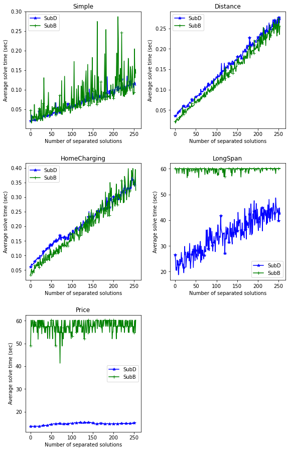
A.3 Further results: Local branching subdomain separation scheme
In Table 6, we report additional performance details for the subproblem solution methods, as in Section 6.3. The new values in the table are defined equivalently as for Table 5.
| Simple | Distance | HomeCharging | LongSpan | Price | ||
|---|---|---|---|---|---|---|
| Solve time (sec) | SepB , all solutions | 46.52 | 2.32 | 1460.34 | 7176.68 | 9045.39 |
| SepB , improving solutions | 0.72 | 1.17 | 8.95 | 7192.53 | 7269.47 | |
| SepD | 1.12 | 1.68 | 4.99 | 7175.38 | 7292.31 | |
| Objective value | SepB , all solutions | 13718.14 | 6635.17 | 8151.72 | 18473.34 | 13439.35 |
| SepB , improving solutions | 13718.14 | 6634.57 | 8151.48 | 18882.63 | 13601.62 | |
| SepD | 13718.14 | 6634.37 | 8151.48 | 18851.94 | 13552.85 | |
| Optimality gap (%) | SepB , all solutions | 0.00 | 0.00 | 0.21 | 21.92 | 22.41 |
| SepB , improving solutions | 0.00 | 0.00 | 0.00 | 13.38 | 18.05 | |
| SepD | 0.00 | 0.00 | 0.00 | 12.47 | 17.47 | |
| Number of nodes | SepB , all solutions | 509.10 | 100.60 | 3061.90 | 1003.45 | 589.73 |
| SepB , improving solutions | 12.75 | 73.95 | 216.35 | 2654.30 | 1117.95 | |
| SepD | 10.00 | 64.10 | 170.80 | 4273.90 | 1592.75 | |
| Average lazy cut time (sec) | SepB , all solutions | 0.05 | 0.09 | 0.16 | 8.93 | 33.00 |
| SepB , improving solutions | 0.05 | 0.09 | 0.13 | 9.13 | 31.90 | |
| SepD | 0.06 | 0.10 | 0.17 | 9.05 | 33.47 | |
| Number of lazy cuts | SepB , all solutions | 9.50 | 3.25 | 11.65 | 23.85 | 23.15 |
| SepB , improving solutions | 7.90 | 3.35 | 11.00 | 68.90 | 47.50 | |
| SepD | 11.45 | 10.05 | 9.40 | 42.10 | 41.35 | |
| Average user cut time (sec) | SepB , all solutions | 0.03 | 0.01 | 0.08 | 3.76 | 12.16 |
| SepB , improving solutions | 0.01 | 0.01 | 0.02 | 1.01 | 3.01 | |
| SepD | 0.01 | 0.00 | 0.01 | 0.33 | 0.95 | |
| Number of user cuts | SepB , all solutions | 652.95 | 23.45 | 2880.55 | 736.65 | 255.12 |
| SepB , improving solutions | 5.70 | 9.70 | 50.80 | 820.25 | 228.80 | |
| SepD | 6.55 | 5.80 | 21.15 | 834.70 | 227.55 | |
| Number of diversified subproblems | SepB , all solutions | 662.45 | 26.70 | 2892.20 | 760.50 | 278.27 |
| SepB , improving solutions | 13.60 | 13.05 | 61.80 | 889.15 | 276.30 | |
| SepD | 18.00 | 15.85 | 30.55 | 876.80 | 268.90 | |
| Number of restricted subproblems | SepB , all solutions | 1424.90 | 98.25 | 13127.65 | 4838.15 | 1708.62 |
| SepB , improving solutions | 31.25 | 41.60 | 195.60 | 4783.15 | 1338.45 | |
| SepD | 87.75 | 101.95 | 170.40 | 6773.35 | 1973.20 | |
| Solve time, LP (sec) | SepB , all solutions | 0.00 | 0.01 | 0.01 | 0.05 | 0.24 |
| SepB , improving solutions | 0.00 | 0.00 | 0.00 | 0.05 | 0.27 | |
| SepD | 0.00 | 0.01 | 0.01 | 0.14 | 0.62 | |
| Number of user-created branches | SepB , all solutions | 654.70 | 27.00 | 2887.90 | 741.20 | 260.38 |
| SepB , improving solutions | 2.20 | 4.70 | 6.70 | 12.40 | 9.30 |