Accelerated Gibbs sampling of normal distributions using matrix splittings and polynomials
Abstract
Standard Gibbs sampling applied to a multivariate normal distribution with a specified precision matrix is equivalent in fundamental ways to the Gauss-Seidel iterative solution of linear equations in the precision matrix. Specifically, the iteration operators, the conditions under which convergence occurs, and geometric convergence factors (and rates) are identical. These results hold for arbitrary matrix splittings from classical iterative methods in numerical linear algebra giving easy access to mature results in that field, including existing convergence results for antithetic-variable Gibbs sampling, REGS sampling, and generalizations. Hence, efficient deterministic stationary relaxation schemes lead to efficient generalizations of Gibbs sampling. The technique of polynomial acceleration that significantly improves the convergence rate of an iterative solver derived from a symmetric matrix splitting may be applied to accelerate the equivalent generalized Gibbs sampler. Identicality of error polynomials guarantees convergence of the inhomogeneous Markov chain, while equality of convergence factors ensures that the optimal solver leads to the optimal sampler. Numerical examples are presented, including a Chebyshev accelerated SSOR Gibbs sampler applied to a stylized demonstration of low-level Bayesian image reconstruction in a large 3-dimensional linear inverse problem.
keywords:
and
1 Introduction
The Metropolis-Hastings algorithm for MCMC was introduced to main-stream statistics around 1990 (Robert and Casella, 2011), though prior to that the Gibbs sampler provided a coherent approach to investigating distributions with Markov random field structure (Turčin, 1971; Grenander, 1983; Geman and Geman, 1984; Gelfand and Smith, 1990; Besag and Green, 1993; Sokal, 1993). The Gibbs sampler may be thought of as a particular Metropolis-Hastings algorithm that uses the conditional distributions as proposal distributions, with acceptance probability always equal to 1 (Geyer, 2011).
In statistics the Gibbs sampler is popular because of ease of implementation (see, e.g., Roberts and Sahu, 1997), when conditional distributions are available in the sense that samples may be drawn from the full conditionals. However, the Gibbs sampler is not often presented as an efficient algorithm, particularly for massive models. In this work we show that generalized and accelerated Gibbs samplers are contenders for the fastest sampling algorithms for normal target distributions, because they are equivalent to the fastest algorithms for solving systems of linear equations.
Almost all current MCMC algorithms, including Gibbs samplers, simulate a fixed transition kernel that induces a homogeneous Markov chain that converges geometrically in distribution to the desired target distribution. In this aspect, modern variants of the Metropolis-Hastings algorithm are unchanged from the Metropolis algorithm as first implemented in the 1950’s. The adaptive Metropolis algorithm of Haario et al. (2001) (see also Roberts and Rosenthal, 2007) is an exception, though it converges to a geometrically convergent Metropolis-Hastings algorithm that bounds convergence behaviour.
We focus on the application of Gibbs sampling to drawing samples from a multivariate normal distribution with a given covariance or precision matrix. Our concern is to develop generalized Gibbs samplers with optimal geometric, or better than geometric, distributional convergence by drawing on ideas in numerical computation, particularly the mature field of computational linear algebra. We apply the matrix-splitting formalism to show that fixed-scan Gibbs sampling from a multivariate normal is equivalent in fundamental ways to the stationary linear iterative solvers applied to systems of equations in the precision matrix.
Stationary iterative solvers are now considered to be very slow precisely because of their geometric rate of convergence, and are no longer used for large systems. However, they remain a basic building block in the most efficient linear solvers. By establishing equivalence of error polynomials we provide a route whereby acceleration techniques from numerical linear algebra may be applied to Gibbs sampling from normal distributions. The fastest solvers employ non-stationary iterations, hence the equivalent generalized Gibbs sampler induces an inhomogeneous Markov chain. Explicit calculation of the error polynomial guarantees convergence, while control of the error polynomial gives optimal performance.
The adoption of the matrix splitting formalism gives the following practical benefits in the context of fixed-scan Gibbs sampling from normal targets:
-
1.
a one-to-one equivalence between generalized Gibbs samplers and classical linear iterative solvers;
-
2.
rates of convergence and error polynomials for the Markov chain induced by a generalized Gibbs sampler;
-
3.
acceleration of the Gibbs sampler to induce an inhomogeneous Markov chain that achieves the optimal error polynomial, and hence has optimal convergence rate;
-
4.
numerical estimates of convergence rate of the Gibbs sampler in a single chain and a priori estimates of number of iterations to convergence;
-
5.
access to preconditioning, whereby the sampling problem is transformed into an equivalent problem for which the accelerated Gibbs sampler has improved convergence rate.
Some direct linear solvers have already been adapted to sampling from multivariate normal distributions, with Rue (2001) demonstrating the use of solvers based on Cholesky factorization to allow computationally efficient sampling. This paper extends the connection to the iterative linear solvers. Since iterative methods are the most efficient for massive linear systems, the associated samplers will be the most efficient for very high dimensional normal targets.
1.1 Context and overview of results
The Cholesky factorization is the conventional way to produce samples from a moderately sized multivariate normal distribution (Rue, 2001; Rue and Held, 2005), and is also the preferred method for solving moderately sized linear systems. For large linear systems, iterative solvers are the methods of choice due to their inexpensive cost per iteration, and small computer memory requirements.
Gibbs samplers applied to normal distributions are essentially identical to stationary iterative methods from numerical linear algebra. This connection was exploited by Adler (1981), and independently by Barone and Frigessi (1990), who noted that the component-wise Gibbs sampler is a stochastic version of the Gauss-Seidel linear solver, and accelerated the Gibbs sampler by introducing a relaxation parameter to implement the stochastic version of the successive over-relaxation (SOR) of Gauss-Seidel. This pairing was further analyzed by Goodman and Sokal (1989).
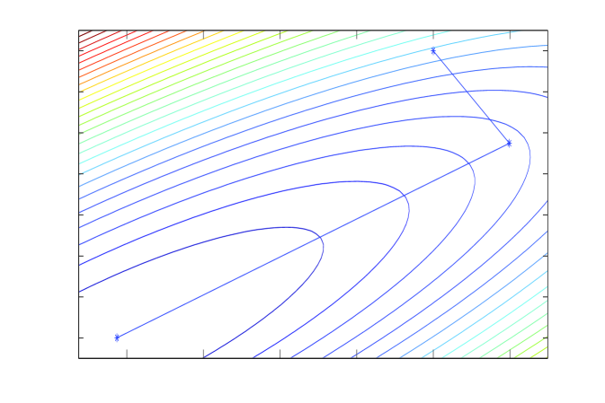
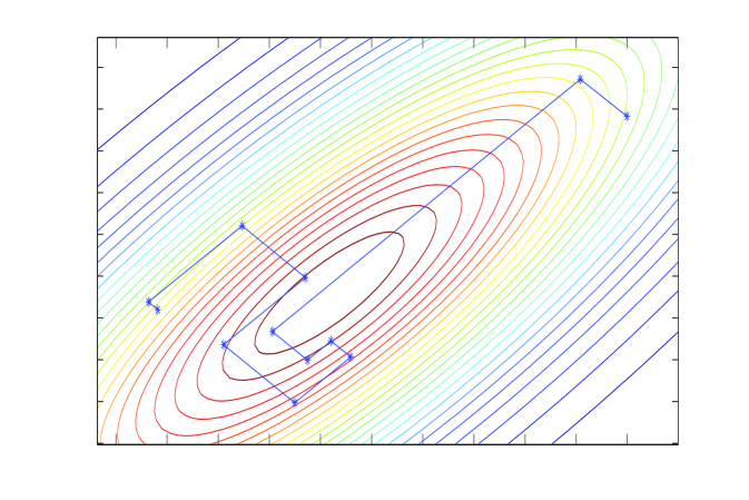
This equivalence is depicted in panels A and B of Figure 1. Panel B shows the contours of a normal density , and a sequence of coordinate-wise conditional samples taken by the Gibbs sampler applied to . Panel A shows the contours of the quadratic minus and the Gauss-Seidel sequence of coordinate optimizations111Gauss-Seidel optimization was rediscovered by Besag (1986) as iterated conditional modes., or, equivalently, solves of the normal equations . Note how in Gauss-Seidel the step sizes decrease towards convergence, which is a tell-tale sign that convergence (in value) is geometric. In Section 4 we will show that the iteration operator is identical to that of the Gibbs sampler in panel B, and hence the Gibbs sampler also converges geometrically (in distribution). Slow convergence of these algorithms is usually understood in terms of the same intuition; high correlations correspond to long narrow contours, and lead to small steps in coordinate directions and many iterations being required to move appreciably along the long axis of the target function.
Solving
Sampling from
A: Gauss-Seidel
B: Gibbs
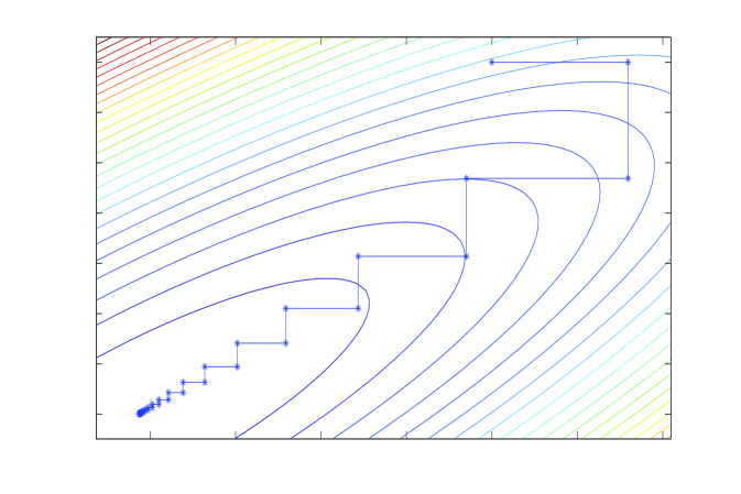
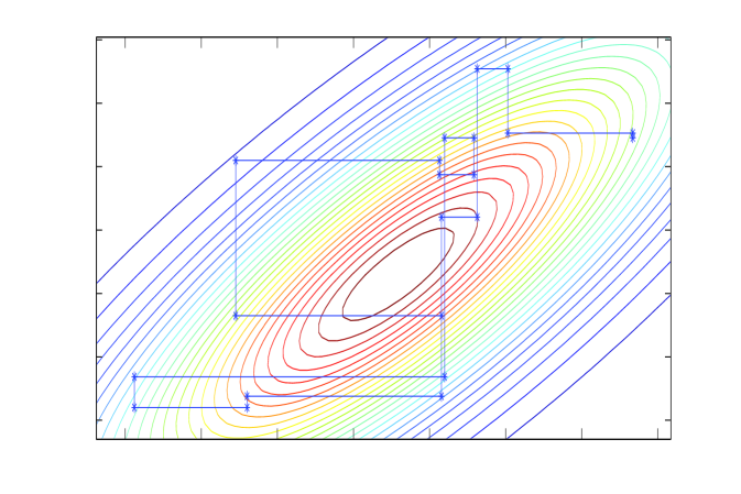 C: Chebyshev-SSOR
D: Chebyshev-SSOR sampler
 E: CG
F: CG Gibbs
Roberts and Sahu (1997) considered forward then backward sweeps of coordinate-wise Gibbs sampling, with relaxation parameter, to give a sampler they termed the REGS sampler. This is a stochastic version of the symmetric-SOR (SSOR) iteration, which comprises forward then backward sweeps of SOR.
The equality of iteration operators and error polynomials, for these pairs of fixed-scan Gibbs samplers and iterative solvers, allows existing convergence results in numerical analysis texts (for example Axelsson, 1996; Golub and Loan, 1989; Nevanlinna, 1993; Saad, 2003; Young, 1971) to be used to establish convergence results for the corresponding Gibbs sampler. Existing results for rates of distributional convergence by fixed-sweep Gibbs samplers (Adler, 1981; Barone and Frigessi, 1990; Liu et al., 1995; Roberts and Sahu, 1997) may be established this way.
The methods of Gauss-Seidel, SOR, and SSOR, give stationary linear iterations that were used as linear solvers in the 1950’s, and are now considered very slow. The corresponding fixed-scan Gibbs samplers are slow for precisely the same reason. The last fifty years has seen an explosion of theoretical results and algorithmic development that have made linear solvers faster and more efficient, so that for large problems, stationary methods are used as preconditioners at best, while the method of preconditioned conjugate gradients, GMRES, multigrid, or fast-multipole methods are the current state-of-the-art for solving linear systems in a finite number of steps (Saad and van der Vorst, 2000).
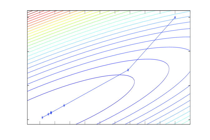
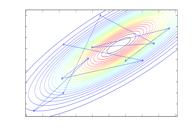
Linear iterations derived from a symmetric splitting may be sped up by polynomial acceleration, particularly Chebyshev acceleration that results in optimal error reduction amongst methods that have a fixed non-stationary iteration structure (Fox and Parker, 1968; Axelsson, 1996). The Chebyshev accelerated SSOR solver and corresponding Chebyshev accelerated SSOR sampler (Fox and Parker, 2014) are depicted in panels C and D of Figure 1. Both the solver and sampler take steps that are more aligned with the long axis of the target, compared to the coordinate-wise algorithms, and hence achieve faster convergence. However, the step size of Chebyshev-SSOR solving still decreases towards convergence, and hence convergence for both solver and sampler is still asymptotically geometric, albeit with much improved rate.
Fox and Parker (2014) considered point-wise convergence of the mean and variance of a Gibbs SSOR sampler accelerated by Chebyshev polynomials. In this paper we prove convergence in distribution for Gibbs samplers corresponding to any matrix splitting and accelerated by any polynomial that is independent of the Gibbs iterations. We then apply a polynomial accelerated sampler to solve a massive Bayesian linear inverse problem that is infeasible to solve using conventional techniques.
Chebyshev acceleration requires estimates of the extreme eigenvalues of the error operator, which we obtain via a conjugate-gradient (CG) algorithm at no significant computational cost (Meurant, 2006). The CG algorithm itself may be adapted to sample from normal distributions; the CG solver and corresponding sampler, depicted in panels E and F of Figure 1, were analysed by Parker and Fox (2012) and is discussed in the supplementary material.
1.2 Structure of the paper
In Section 2 we review efficient methods for sampling from normal distributions, highlighting Gibbs sampling in various algorithmic forms. Standard results for stationary iterative solvers are presented in Section 3. Theorems in Section 4 establish equivalence of convergence and convergence factors for iterative solvers and Gibbs samplers. Application of polynomial acceleration methods to linear solvers and Gibbs sampling is given in Section 5, including a proof of convergence of the first and second moments of a polynomial accelerated sampler. Numerical verification of convergence results is presented in Section 6.
2 Sampling from multivariate normal distributions
We consider the problem of sampling from an -dimensional normal distribution defined by the mean -vector , and the symmetric and positive definite (SPD) covariance matrix . Since if then , it often suffices to consider drawing samples from normal distributions with zero mean. An exception is when is defined implicitly, which we discuss in section 4.1.
In Bayesian formulations of inverse problems that use a GMRF as a prior distribution, typically the precision matrix is explicitly modeled and available (Rue and Held, 2005; Higdon, 2006), perhaps as part of a hierarchical model (Banerjee et al., 2003). Typically then the precision matrix (conditioned on hyperparameters) is large though sparse, if the neighborhoods specifying conditional independence are small. We are particularly interested in this case, and throughout the paper will focus on sampling from when is sparse and large, or when some other property makes operating by easy, i.e., one can evaluate for any vector .
Standard sampling methods for moderately sized normal distributions utilize the Cholesky factorization (Rue, 2001; Rue and Held, 2005) since it is fast, incurring approximately floating point operations (flops) and is backwards stable (Watkins, 2002). Samples can also be drawn using the more expensive eigen-decomposition (Rue and Held, 2005), that costs approximately flops, or more generally using mutually conjugate vectors (Fox, 2008; Parker and Fox, 2012). For stationary Gaussian random fields defined on the lattice, Fourier methods can lead to efficient sampling for large problems (Gneiting et al., 2005).
Algorithm 1 shows the steps for sampling from using Cholesky factorization, when the
covariance matrix is available (Neal, 1997; MacKay, 2003; Higdon, 2006).
When the precision matrix is available, a sample may be drawn using Algorithm 2 given by Rue (2001) (see also Rue and Held, 2005).
The computational cost of Algorithm 2 depends on the bandwidth of , that also bounds the bandwidth of the Cholesky factor . For a bandwidth , calculation of the Cholesky factorization requires flops, which provides savings over the full-bandwidth case when (Golub and Loan, 1989; Rue, 2001; Watkins, 2002). For GMRF’s defined over 2-dimensional domains, the use of a bandwidth reducing permutation often leads to substantial computational savings (Rue, 2001; Watkins, 2002). In 3-dimensions and above, typically no permutation exists that can significantly reduce the bandwidth below , hence the cost of sampling by Cholesky factoring is at least flops. Further, Cholesky factorizing requires that the precision matrix and the Cholesky factor be stored in computer memory, which can be prohibitive for large problems. In Section 6 we give an example of sampling from a large GMRF for which Cholesky factorization is prohibitively expensive.
2.1 Gibbs sampling from a normal distribution
Iterative samplers, such as Gibbs, are an attractive option when drawing samples from high dimensional multivariate normal distributions due to their inexpensive cost per iteration and small computer memory requirements (only vectors of size need be stored). If the precision matrix is sparse with non-zero elements, then, regardless of the bandwidth, iterative methods cost only about flops per iteration, which is comparable with sparse Cholesky factorizations. However, when the bandwidth is , the cost of the Cholesky factorization is high at flops, while iterative methods maintain their inexpensive cost per iteration. Iterative methods are then preferable when requiring significantly fewer than iterations for adequate convergence. In the examples presented in section 6 we find that iterations give convergence to machine precision, so the iterative methods are preferable for large problems.
2.1.1 Componentwise formulation
One of the simplest iterative sampling methods is the component-sweep Gibbs sampler (Geman and Geman, 1984; Gelman et al., 1995; Gilks et al., 1996; Rue and Held, 2005). Let denote a vector in terms of its components, and let be an precision matrix with elements . One sweep over all components can be written as in Algorithm 3 (Barone and Frigessi, 1990), showing that the algorithm can be implemented using vector and scalar operations only, and storage or inversion of the precision matrix is not required.
The index may be omitted (and with ‘’ interpreted as assignment) to give an algorithm that can be evaluated in place, requiring minimal storage.
2.1.2 Matrix formulation
One iteration in Algorithm 3 consists of a sweep over all components of in sequence. The iteration can be written succinctly in the matrix form (Goodman and Sokal, 1989)
| (1) |
where , , and is the strictly lower triangular part of . This equation makes clear that the computational cost of each sweep is about flops, when is dense, due to multiplication by the triangular matrices and , and flops when is sparse.
Extending this formulation to sweeps over any other fixed sequence of coordinates is achieved by putting in place of for some permutation matrix . The use of random sweep Gibbs sampling has also been suggested (Amit and Grenander, 1991; Fishman, 1996; Liu et al., 1995; Roberts and Sahu, 1997), though we do not consider that here.
2.1.3 Convergence
If the iterates in (1) converge in distribution to a distribution which is independent of the starting state , then the sampler is convergent, and we write
It is well known that the iterates in the Gibbs sampler (1) converge in distribution geometrically to (Roberts and Sahu, 1997). We consider geometric convergence in detail in Section 4.
3 Linear stationary iterative methods as linear equation solvers
Our work draws heavily on existing results for stationary linear iterative methods for solving linear systems. Here we briefly review the main results that we will use.
Consider a system of linear equations written as the matrix equation
| (2) |
where is a given nonsingular matrix and is a given -dimensional vector. The problem is to find an -dimensional vector satisfying equation (2). Later we will consider the case where is symmetric positive definite (SPD) as holds for covariance and precision matrices (Feller, 1968).
3.1 Matrix splitting form of stationary iterative algorithms
A common class of methods for solving (2) are the linear iterative methods based on a splitting of into . The matrix splitting is the standard way of expressing and analyzing linear iterative algorithms, following its introduction by Varga (1962). The system (2) is then transformed to or, if is nonsingular, The iterative methods use this equation to compute successively better approximations to the solution using the iteration step
| (3) |
We follow the standard terminology used for these methods (see e.g. Axelsson, 1996; Golub and Loan, 1989; Saad, 2003; Young, 1971). Such methods are termed linear stationary iterative methods (of the first degree); they are stationary222This use of stationary corresponds to the term homogeneous when referring to a Markov chain. It is not to be confused with a stationary distribution that is invariant under the iteration. Later we will develop non-stationary iterations, inducing a non-homogeneous Markov chain that will, however, preserve the target distribution at each iterate. because the iteration matrix and the vector do not depend on . The splitting is symmetric when both and are symmetric matrices. The iteration, and splitting, is convergent if tends to a limit independent of , the limit being (see, e.g. (Young, 1971, Theorem 5.2)).
The iteration (3) is often written in the residual
form
so that convergence may be monitored in terms of the norm of the
residual vector, and emphasizes that is acting
as an approximation to , as in
Algorithm 4.
In computational algorithms it is important to note that the symbol is interpreted as “solve the system for ” rather than “form the inverse of and multiply by ” since the latter is much more computationally expensive (about flops (Watkins, 2002)). Thus, the practicality of a splitting depends on the ease with which one can solve for any vector .
3.1.1 The Gauss-Seidel algorithm
Many splittings of the matrix use the terms in the expansion where is the strictly lower triangular part of , is the diagonal of , and is the strictly upper triangular part.
For example, choosing (so ) allows to be solved by “forward substitution” (at a cost of flops when is dense), and hence does not require inversion or Gauss-elimination of (which would cost flops when is dense). Using this splitting in Algorithm 4 results in the Gauss-Seidel iterative algorithm. When is symmetric, , and the Gauss-Seidel iteration can be written as
| (4) |
Just as we pointed out for the Gibbs sampler, variants of the Gauss-Seidel algorithm such as “red-black” coordinate updates (Saad, 2003), may be written in this form using a suitable permutation matrix.
The component-wise form of the Gauss-Seidel algorithm can be written in ‘equation’ form just as the Gibbs sampler (1) was in Algorithm 3. The component-wise form emphasizes that Gauss-Seidel can be implemented using vector and scalar operations only, and neither storage nor inversion of the splitting is required.
3.2 Convergence
A fundamental theorem of linear stationary iterative methods states that the splitting , where is nonsingular, is convergent (i.e., for any ) if and only if , where denotes the spectral radius of a matrix (Young, 1971, Theorem 3.5.1). This characterization is often used as a definition (Axelsson, 1996; Golub and Loan, 1989; Saad, 2003).
The error at step is , where . It follows that
| (5) |
and hence the asymptotic average reduction in error per iteration is the multiplicative factor
| (6) |
(Axelsson, 1996, p. 166). In numerical analysis this is called the (asymptotic average) convergence factor (Axelsson, 1996; Saad, 2003). Later, we will show that this is exactly the same as the quantity called the geometric convergence rate in the statistics literature (see e.g. Robert and Casella, 1999), for the equivalent Gibbs sampler. We will use the term ‘convergence factor’ throughout this paper to avoid a clash of terminology, since in numerical analysis the rate of convergence is minus the log of the convergence factor (see e.g. Axelsson, 1996, p. 166).
3.3 Common matrix splittings
We now present the matrix splittings corresponding to some common stationary linear iterative solvers, with details for the case where is symmetric, as holds for precision or covariance matrices.
We have seen that the Gauss-Seidel iteration uses the splitting and . Gauss-Seidel is one of the simplest splittings and solvers, but is also quite slow. Other splittings have been developed, though the speed of each method is often problem specific. Some common splittings are shown in Table 1, listed with, roughly, greater speed downwards. Speed of convergence in a numerical example is presented later in Section 6.
splitting convergence Richardson (R) Jacobi (J) strictly diagonally dominant Gauss-Seidel (GS) always SOR SSOR
The method of successive over-relaxation (SOR) uses the splitting
| (7) |
in which is a relaxation parameter chosen with . SOR with is Gauss-Seidel. For optimal values of such that , SOR is an accelerated Gauss-Seidel iteration. Unfortunately, there is no closed form for the optimal value of for an arbitrary matrix , and the interval of values of which admits accelerated convergence can be quite narrow (Young, 1971; Golub and Loan, 1989; Saad, 2003).
The symmetric-SOR method (SSOR) incorporates both a forward and backward sweep of SOR so that if is symmetric then the splitting is symmetric (Golub and Loan, 1989; Saad, 2003),
| (8) |
We will make use of symmetric splittings in conjunction with polynomial acceleration in Section 5.
When the matrix is dense, Gauss-Seidel and SOR cost about flops per iteration, with due to multiplication by the matrix (in order to calculate the residual) and another for the forward substitution to solve . Richardson incurs no cost to solve , while a solve with the diagonal Jacobi matrix incurs flops. Iterative methods are particularly attractive when the matrix is sparse, since then the cost per iteration is only flops.
4 Equivalence of stationary linear solvers and Gibbs samplers
We first consider the equivalence between linear solvers and stochastic iterations in the case where the starting state and noise are not necessarily normally distributed, then in Section 4.2 et seq. we restrict consideration to normal distributions.
4.1 General noise
The striking similarity between the Gibbs sampler (1) and the Gauss-Seidel iteration (4) is no coincidence. It is an example of a general equivalence between the stationary linear solver derived from a splitting and the associated stochastic iteration used as a sampler. We will make explicit the equivalence in the following theorems and corollary. In the first theorem we show that a splitting is convergent (in the sense of stationary iterative solvers) if and only if the associated stochastic iteration is convergent in distribution.
Theorem 1
Let be a splitting with invertible, and let be some fixed probability distribution with zero mean and fixed non-zero covariance. For any fixed vector , and random vectors , , the stationary linear iteration
| (9) |
converges, with as whatever the initial vector , if and only if there exists a distribution such that the stochastic iteration
| (10) |
converges in distribution to , with as whatever the initial state .
Proof. If the linear iteration (9) converges, then (Thm 3-5.1 in Young, 1971). Hence there exists a unique distribution with (Theorem 2.3.18-4 of Duflo, 1997), which shows necessity. Conversely, if the linear solver does not converge to a limit independent of for some , that also holds for and hence initializing the sampler with yields which does not converge to a value independent of . Sufficiency holds by the contrapositive.
Convergence of the stochastic iteration (10) could also be established via the more general theory of Diaconis and Freedman (1999) that allows the iteration operator to be random, with convergence in distribution guaranteed when is contracting on average; see Diaconis and Freedman (1999) for details.
The following theorem shows how to design the noise distribution so that the limit distribution has a desired mean and covariance .
Theorem 2
Let be SPD, be a convergent splitting, a fixed vector, and a fixed probability distribution with finite mean and non-zero covariance . Consider the stochastic iteration (10) where , . Then, whatever the starting state , the following are equivalent:
-
1.
and
-
2.
the iterates converge in distribution to some distribution that has mean and covariance matrix ; in particular and as .
Proof. Appendix A.1.
Additionally, the mean and covariance converge geometrically, with convergence factors given by the convergence factors for the linear iterative method, as established in the following corollary.
Corollary 3
The first and second moments of iterates in the stochastic iteration in Theorem 2 converge geometrically. Specifically, with convergence factor and with convergence factor .
Proof. Appendix A.1.
Note that the matrix splitting has allowed an explicit construction of the noise covariance to give a desired precision matrix of the target distribution. We see from Theorem 2 that the stochastic iteration may be designed to converge to a distribution with non-zero target mean, essentially by adding the deterministic iteration (9) to the stochastic iteration (10). This is particularly useful when the mean is defined implicitly via solving a matrix equation. In cases where the mean is known explicitly, the mean may be added after convergence of the stochastic iteration with zero mean, giving an algorithm with faster convergence since the covariance matrix converges with factor (this was also noted by Barone et al., 2002). Convergence in variance for non-normal targets was considered in Fox and Parker (2014).
Using Theorems 1 and 2, and Corollary 3 we can draw on the vast literature in numerical linear algebra on stationary linear iterative methods to find random iterations that are computationally efficient and provably convergent in distribution with desired mean and covariance. In particular, results in Amit and Grenander (1991); Barone and Frigessi (1990); Galli and Gao (2001), Roberts and Sahu (1997), and Liu et al. (1995) are special cases of the general theory of matrix splittings presented here.
4.2 Sampling from normal distributions using matrix splittings
We now restrict attention to the case of normal target distributions.
Corollary 4
If in Theorem 2 we set , for some non-zero covariance matrix , then, whatever the starting state , the following are equivalent: (i) ; (ii) where .
Proof. Since is normal, then in Theorem 2 is normal. Since a normal distribution is sufficiently described by its first two moments, the corollary follows.
Using Corollary 4, we found normal sampling algorithms corresponding to some common stationary linear solvers. The results are given in Table 2.
Sampler Richardson Jacobi Gibbs (Gauss-Seidel) SOR SSOR (REGS)
A sampler corresponding to a convergent splitting is implemented in Algorithm 5.
The assignment in Algorithm 5 can be replaced by the slightly more expensive steps and , which allows monitoring of the residual, and emphasizes the equivalence with the stationary linear solver in Algorithm 4. Even though convergence may not be diagnosed by a decreasing norm of the residual, lack of convergence can be diagnosed when the residual diverges in magnitude. In practice, the effective convergence factor for a sampler may be calculated by solving the linear system (2) (perhaps with a random right hand side) using the iterative solver derived from the splitting and monitoring the decrease in error to evaluate the asymptotic average convergence factor using equation (6). By Corollary 3, this estimates the convergence factor for the sampler.
The practicality of a sampler derived from a convergent splitting depends on the ease with which one can solve for any (as for the stationary linear solver) and also the ease of drawing iid noise vectors from . Sampling the noise vector is simple when a matrix square root, such as the Cholesky factorization, of is cheaply available. Thus, a sampler is at least as expensive as the corresponding linear solver since, in addition to operations in each iteration, the sampler must factor the matrix . For the samplers listed in Table 2 it is interesting that the simpler the splitting, the more complicated is the variance of the noise. Neither Richardson nor Jacobi splittings give useful sampling algorithms since the difficulty of sampling the noise vector is no less than the original task of sampling from . The Gauss-Seidel splitting, giving the usual Gibbs sampler, is at a kind of sweet spot, where solving equations in is simple while the required noise variance is diagonal, so posing a simple sampling problem.
The SOR stationary sampler uses the SOR splitting and in (7) for and the noise vector (Table 2). This sampler was introduced by Adler (1981), rediscovered by Barone and Frigessi (1990), and has been studied extensively (Barone et al., 2002; Galli and Gao, 2001; Liu et al., 1995; Neal, 1998; Roberts and Sahu, 1997). For , the SOR sampler is a Gibbs (Gauss-Seidel) sampler. For values of such that ), the SOR-sampler is an accelerated Gibbs sampler. As for the linear solver, implementation of the Gibbs and SOR samplers by Algorithm 5 requires multiplication by the upper triangular and forward substitution with respect to at a cost of flops. In addition, these samplers must take the square root of the diagonal matrix at a mere cost of flops.
Implementation of an SSOR sampler instead of a Gibbs or SOR sampler is advantageous
since the Markov chain is reversible
(Roberts and
Sahu, 1997). SSOR sampling uses the symmetric-SOR splitting and in (8).
The SSOR stationary sampler is most easily implemented by forward and backward
SOR sampling sweeps as in Algorithm 6, so the matrices
and need never be explicitly formed.
We first encountered restricted versions of Corollary 4 for normal distributions in Amit and Grenander (1991) and in Barone and Frigessi (1990) where geometric convergence of the covariance matrices was established for the Gauss-Seidel and SOR splittings. These and the SSOR splitting were investigated in Roberts and Sahu (1997) (who labelled the sampler REGS).
Corollary 4 and Table 1 show that the Gibbs, SOR and SSOR samplers converge for any SPD precision matrix . This summarizes results in Barone and Frigessi (1990); Galli and Gao (2001) and the deterministic sweeps investigated in Amit and Grenander (1991); Roberts and Sahu (1997); Liu et al. (1995). Corollary 4 generalizes these results for any matrix splitting by guaranteeing convergence of the random iterates (10) to with convergence factor (or if ).
5 Non-stationary iterative methods
5.1 Acceleration of linear solvers by polynomials
A common scheme in numerical linear algebra for accelerating a stationary method when and are symmetric is through the use of polynomial preconditioners (Axelsson, 1996; Golub and Loan, 1989; Saad, 2003). Equation (5) shows that after steps the error in the stationary method is a order polynomial of the matrix . The idea behind polynomial acceleration is to implicitly implement a different order polynomial such that . The coefficients of are functions of a set of acceleration parameters , introduced by the second order iteration
| (11) |
At the first step, and . Setting for every yields a basic un-accelerated stationary method. The accelerated iteration in (11) is implemented at a negligible increase in cost of flops per iteration (due to scalar-vector multiplication and vector addition) over the corresponding stationary solver (3).
It can be shown that (e.g., Axelsson (1996)) that the order polynomial generated recursively by the second order non-stationary linear solver (11) is
| (12) |
This polynomial acts on the error by , which can be compared directly to (5).
When estimates of the extreme eigenvalues and of are available ( and are real when and are symmetric), then the coefficients can be chosen to generate the scaled Chebyshev polynomials , which give optimal error reduction at every step. The Chebyshev acceleration parameters are
| (13) |
where and (Axelsson, 1996). Note that these parameters are independent of the iterates . Since is required to be symmetric, applying Chebyshev acceleration to SSOR is a common pairing; its effectiveness as a linear solver is shown later in Table 3.
Whereas the stationary methods converge with asymptotic average convergence factor , the convergence factor for the Chebyshev method depends on . Specifically the scaled Chebyshev polynomial minimizes over all order polynomials , with
| (14) |
Since the error at the step of a Chebyshev accelerated linear solver is , then the asymptotic convergence factor is bounded above by
| (15) |
(p.181 Axelsson, 1996). Since , the polynomial accelerated scheme is guaranteed to converge even if the original splitting was not convergent. Further, the convergence factor of the stationary iterative solver is bounded below by (see e.g. Axelsson, 1996, Thm 5.9). Since (except when in which case ), polynomial acceleration always reduces the convergence factor, so justifies the term acceleration. The Chebyshev accelerated iteration (11) is amenable to preconditioning that reduces the condition number, and hence reduces , such as incomplete Cholesky factorization or graphical methods (Axelsson, 1996; Saad, 2003). Axelsson also shows that after
| (16) |
iterations of the Chebyshev solver, the error reduction is for some real number and any (Axelsson, 1996, eqn 5.32).
5.2 Acceleration of Gibbs sampling by polynomials
Any acceleration scheme devised for a stationary linear solver is a candidate for accelerating convergence of a Gibbs sampler. For example, consider the second order stochastic iteration
| (17) |
analogous to the linear solver in (11) but now the vector has been replaced by a random vector . The equivalence between polynomial accelerated linear solvers and polynomial accelerated samplers is made clear in the next three theorems.
Theorem 5
Let be SPD and be a symmetric splitting. Consider a set of independent noise vectors with moments
such that , , , and . If the polynomial accelerated linear solver (11) converges to with a set of parameters , that are independent of , then the polynomial accelerated stochastic iteration (17) converges in distribution to a distribution with mean and covariance matrix . Furthermore, if the are normal, then
Proof. Appendix A.2.
Given a second order linear solver (11) that converges, Theorem 5 makes clear how to construct a second order sampler (17) that is guaranteed to converge. The next Corollary shows that the polynomial that acts on the linear solver error is the same polynomial that acts on the errors in the first and second moments of the sampler, and respectively. In other words, the convergence factors for a polynomial accelerated solver and sampler are the same.
Corollary 6
Proof. Appendix A.2.
Corollary 6 allows a direct comparison of the convergence factor for a polynomial accelerated sampler (, or if ) to the convergence factor given previously for the corresponding un-accelerated stationary sampler (, or if ). In particular, given a second order linear solver with accelerated convergence compared to the corresponding stationary iteration, the corollary guarantees that the second order Gibbs sampler (17) will converge faster than the stationary Gibbs sampler (10).
Just as Chebyshev polynomials are guaranteed to accelerate linear solvers, Corollary 6 assures that Chebyshev polynomials can also accelerate a Gibbs sampler. Using Theorem 5, we derived the Chebyshev accelerated SSOR sampler (Fox and Parker, 2014) by iteratively updating parameters via (13) and then generating a sampler via (17). Explicit implementation details of the Chebyshev accelerated sampler are provided in the supplementary materials. The polynomial accelerated sampler is implemented at a negligible increase in cost of flops per iteration over the cost ( flops) of the SSOR sampler (Algorithm 6). The asymptotic convergence factor is given by the next Corollary, which follows from Corollary 6 and equation (15).
Corollary 7
If the Chebyshev accelerated linear solver converges, then the mean of the corresponding Chebyshev accelerated stochastic iteration (17) converges to with asymptotic convergence factor and the covariance matrix converges to with asymptotic convergence factor .
Corollary 7 and (14) show that a Chebyshev accelerated normal sampler is guaranteed to converge faster than any other acceleration scheme that has the parameters independent of the iterates . This result also shows that the preconditioning ideas presented in section 5.1 to reduce can also be used to speed up Chebyshev accelerated samplers. We do not investigate such preconditioning here.
Corollary 7 and equation (16) suggest that, for any , after iterations the Chebyshev error reduction for the mean is smaller than . But even sooner, after iterations, the Chebyshev error reduction for the variance is predicted to be smaller than (Fox and Parker, 2014).
6 Computed Examples
The iterative sampling algorithms we have investigated are designed for problems where operating by the precision matrix is cheap. A common such case is when the precision matrix is sparse, as occurs when modeling a GMRF with a local neighbourhood structure. Then, typically, the precision matrix has non-zero elements, so direct matrix-vector multiplication has cost. We give two examples of sampling using sparse precision matrices: first, we present a small example where complete diagnostics can be computed for evaluating the quality of convergence; and second, we present a Bayesian linear inverse problem that demonstrates computational feasibility for large problems. The samplers are initialized with in both examples.
6.1 A lattice example ()
A first order locally linear sparse precision matrix , considered by Higdon (2006); Rue and Held (2005), is
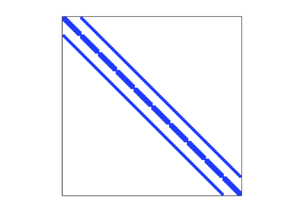
The discrete points are on a regular lattice () over the two dimensional domain . Thus is , and . The sparsity of is shown in the left panel of Figure 2. The scalar is the number of points neighbouring , i.e., with distance from . Although , the number of non-zero elements of is ( in this example). Since the bandwidth of is , a Cholesky factorization costs flops (Rue, 2001) and each iteration of an iterative method costs flops.
To provide a comparison between linear solvers and samplers, we solved the system using linear solvers with different matrix splittings (Table 1), where is fixed and non-zero, all initialized with . The results are given in Table 3. The Richardson method does not converge (DNC) since the spectral radius of the iteration operator is greater than 1. The SOR iteration was run at the optimal relaxation parameter value of . SSOR was run at its optimal value of . Chebyshev accelerated SSOR (Cheby-SSOR), CG accelerated SSOR (CG-SSOR) (both run with ) and CG utilize a different implicit operator for each iteration, and so the spectral radius given in these cases is the geometric mean spectral radius of these operators (estimated using (5)). Even for this small example, Chebyshev acceleration reduces the computational effort required for convergence by about two orders of magnitude, while CG acceleration reduces work by nearly two more orders of magnitude.
solver number of iterations flops Richardson 1 6.8 DNC – Jacobi – .999972 Gauss-Seidel – .999944 SSOR 1.6641 .999724 SOR 1.9852 .985210 1655 Cheby-SSOR 1 .9786 958 Cheby-SSOR 1.6641 .9673 622 CG – .6375 48 CG-SSOR 1.6641 .4471 29 Cholesky – – –
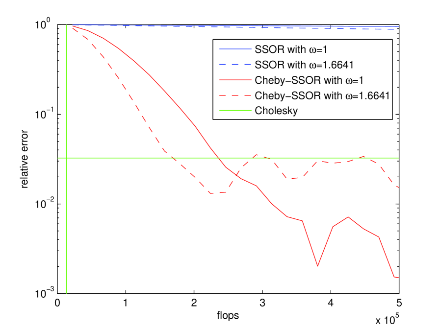
We investigated the following Gibbs samplers: SOR, SSOR, and the Chebyshev accelerated SSOR. These samplers are guaranteed to converge since the corresponding solver converges (Theorem 1). Since the convergence factor for a sampler is equal to the convergence factor for the corresponding solver (Corollaries 3 and 6) then Gibbs samplers implemented with any of the matrix splittings in Table 1 exhibit the same convergence behavior as shown for the linear solvers in Table 3. Convergence of the sample covariance , calculated using samples, is shown in the right panel of Figure 2 that displays the relative error as a function of the flop count. Each sampler iteration costs about flops. This performance is compared to samples constructed by a Cholesky factorization, which cost flops (depicted as the green vertical line in the right panel of Figure 2). Since the sample means were uniformly close to zero, error in the mean is not shown.
The benchmark for evaluation of the of the convergence of the iterative samplers in finite precision is the Cholesky factorization, its relative error is depicted as the green horizontal line in the right panel of Figure 2. For this example, the iterative samplers produce better samples than a Cholesky sampler since the iterative sample covariances become more precise with more computing time.
The geometric convergence in distribution of the un-accelerated SSOR samples to is clear in Figure 2, and even after flops, convergence in distribution has not been attained. This is not surprising based on the large number of iterations () necessary for the same stationary method to converge to a solution of (see Table 3). The accelerated convergence of the Chebyshev polynomial samplers, suggested by the fast convergence of the corresponding linear solvers depicted in Table 3, is also evident in Figure 2, with convergence after flops (76 iterations) for the Cheby-SSOR sampler with optimal relaxation parameter , and the somewhat slower convergence at flops (106 iterations) when .
6.2 A () linear inverse problem in biofilm imaging
We now perform accelerated sampling from a GMRF in 3-dimensions, as a stylized example of estimating a voxel image of a biofilm from confocal scanning laser microscope (CSLM) data (Lewandowski and Beyenal, 2014). This large example illustrates the feasibility of Chebyshev accelerated sampling in large problems for which sampling by Cholesky factorization of the precision matrix is too computationally and memory intensive to be performed on a standard desktop computer.
We consider the problem of reconstructing a voxel image of a bacterial biofilm, i.e., a community of bacteria aggregated together as slime, given a subsampled CSLM data set . For this exercise, we synthesized a ‘true’ image of a m tall ellipsoidal column of biofilm attached to a surface, taking value inside the biofilm column, and outside, in arbitrary units. Similar geometry has been observed experimentally for Pseudomonas aeruginosa biofilms (Swogger and Pitts, 2005), and is also predicted by mathematical models of biofilm growth (Alpkvist and Klapper, 2007). CSLM captures a set of planar ‘images’ at different distances from the bottom of the biofilm where it is attached to a surface. In nature biofilms attach to any surface over which water flows, e.g., human teeth and creek bottoms. Each horizontal planar image in this example is pixels; the distance between pixels in each plane is typically about 1 m, with the exact spatial resolution set by the microscope user. The vertical distance between planar slices in a CSLM image is typically an order of magnitude larger than the horizontal distance between pixels; for this example, the vertical distance between CSLM planes is 10m.
Given the ‘true’ image , we generated synthetic CSLM data by
where the matrix arithmetically averages over 10 pixels in the vertical dimension of , to approximate the point spread function (PSF) of CSLM (Sheppard and Shotton, 1997), and ). The data is displayed in the left panel of Figure 3 as layers of pixels, or ‘slices’, located at the centre of sensitivity of the CSLM, i.e. the centre of the PSF. Thus, the likelihood we consider is .
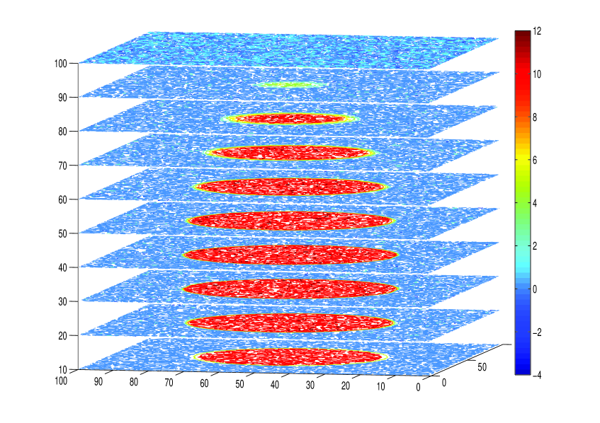
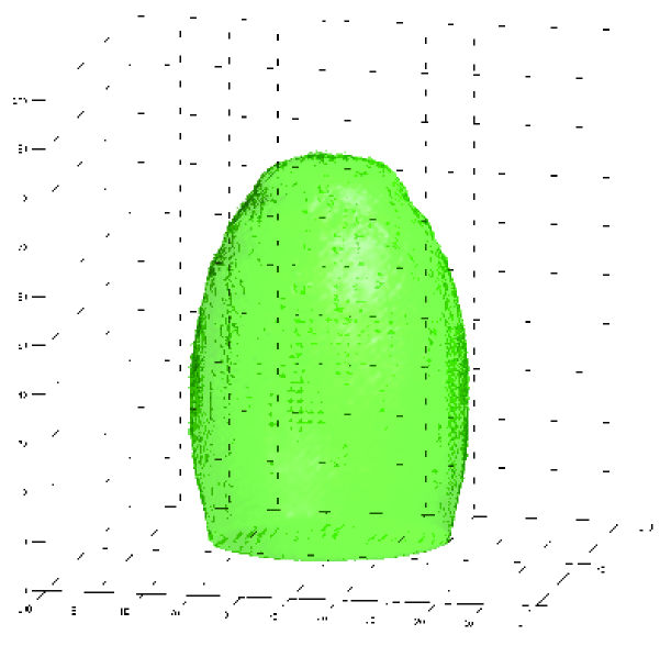
To encapsulate prior knowledge that the bacteria in the biofilm aggregate together we model by the GMRF where the precision matrix models local smoothness of the density of the biofilm and background. We construct the matrix as a sparse inverse of the dense covariance matrix corresponding to the exponential covariance function. This construction uses the relationship between stationary Gaussian random fields and partial differential equations (PDEs) that was noted by Whittle (1954) for the Matérn (or Whittle-Matérn (Guttorp and Gneiting, 2005)) class of covariance functions, that was also exploited by Cui et al. (2011) and Lindgren et al. (2011). Rather than stating the PDE, we find it more convenient to work with the equivalent variational form, in this case (the square of)
where is a continuous stochastic field, is the volume element in the domain and is the surface element on the boundary . This form has Euler-Lagrange equations being the Helmholtz operator with (local) Robin boundary conditions on , induced by the term. In our example we apply the Hessian of this form twice, which can be thought of as squaring the Helmholtz operator. When the quadratic form is written in the operator form , where is the Hessian, the resulting Gaussian random field has density
| (19) |
We chose this operator because the discretized precision matrix is sparse, while the covariance function (after scaling) is close to , having length-scale .
The GMRF over the discrete field is then defined using FEM (finite element method) discretization; we used cubic-elements between nodes at voxel centres in the cubic domain, and tri-linear interpolation from nodal values within each element. To verify this construction we show in Figure 4 contours of the resulting covariance function, between the pixel at the centre of the normalised cubic domain and all other pixels, for length scale . The contours are logarithmically spaced in value, hence the evenly spaced spherical contours show that the covariance indeed has exponential dependence with distance. The contours look correct at the boundaries, indicating that the local Robin boundary conditions333Local boundary conditions are approximate but preserve sparseness. The exact boundary conditions are given by the boundary integral equation for the exterior Helmholtz operator, resulting in a dense block in that is inconvenient for computation (Neumayer, 2011). give the desired covariance function throughout the domain. In contrast, Dirichlet conditions would make the cubic boundary a contour, while Neumann conditions as used by Lindgren et al. (2011) would make contours perpendicular to the cubic boundary; neither of those pure boundary conditions produce the desired covariance function.
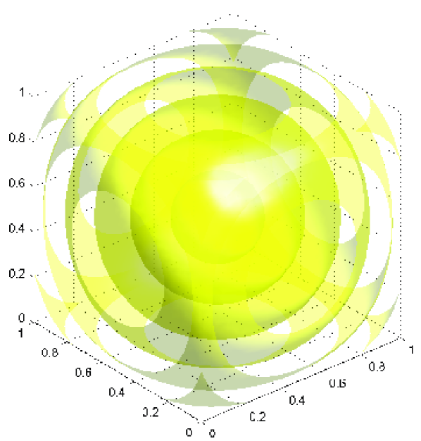
In the deterministic setting, this image recovery problem is an example of a linear inverse problem. In the Bayesian setting, we may write the hierarchical model in the general form
| (20) | |||||
| (21) | |||||
| (22) |
where is a vector of hyperparameters. This stochastic model occurs in many settings (see, e.g., Simpson et al., 2012; Rue and Held, 2005) with being observed data, is a latent field, and is a vector of hyperparameters that parameterize the precision matrices and . The (hyper)prior models uncertainty in covariance of the two random fields.
There are several options for performing sample-based inference on the model (20), (21), (22). Most direct is forming the posterior distribution via Bayes’ rule and implementing Markov chain Monte Carlo (MCMC) sampling, typically employing Metropolis-Hastings dynamics with a random walk proposal on and . Such an algorithm can be very slow due to high correlations within the latent field , and between the latent field and hyperparameters . More efficient algorithms block the latent field, noting that the distribution over given everything else is a multivariate normal, and hence can be sampled efficiently as we have discussed in this paper. Higdon (2006) and Bardsley (2012) utilized this structure, along with conjugate hyperpriors on the components of , to demonstrate a Gibbs sampler that cycled through sampling from the conditional distributions for and components of . When the normalizing constant for is available, up to a multiplicative constant independent of state, a more efficient algorithm is the one block algorithm (Rue and Held, 2005, section 4.1.2) in which a candidate is drawn from a random walk proposal, then a draw , with the joint proposal accepted with the standard Metropolis-Hastings probability. The resulting transition kernel in is in detailed balance with the distribution over , and hence can improve efficiency dramatically. A further improvement can be to perform MCMC directly on as indicated by Simpson et al. (2012), with subsequent independent sampling to facilitate Monte Carlo evaluation of statistics. In each of these schemes, computational cost is dominated by the cost of drawing samples from the large multivariate normal . We now demonstrate that sampling step for this synthetic example.
In our example, the distribution over the image , conditioned on everything else, is the multivariate normal
| (23) |
with precision matrix (cf. Calvetti and Somersalo (2007); Higdon (2006)). For this calculation we used the same covariance matrix as shown above, so in units of the width of the domain, though for sample-based inference one would use samples from the distribution over . The right panel of Figure 3 depicts a reconstructed surface derived from a sample from the conditional distribution in (23) using the Chebyshev polynomial accelerated SSOR sampler. The sampler was initialized with the precision matrix , for all , and relaxation parameter . The contour is at value , after smoothing over voxels, displaying a sample surface that separates regions for which the average over voxel blocks is less than (outside surface) and greater than (inside surface). As can be seen, the surface makes an informative reconstruction of the ellipsoidal phantom.
Using CG, estimates of the extreme eigenvalue of were and . By Corollary 6, the asymptotic convergence factors for the Chebyshev sampler are for the mean and for the covariance matrix. Using this information, equation (16) predicts the number of sampler iterations until convergence. After iterations of the Chebyshev accelerated sampler, it is predicted that the mean error is reduced by ; that is
But even sooner, after only iterations, it is predicted that the covariance error is
Contrast these Chebyshev polynomial convergence results to the performance of the non-accelerated stationary SSOR sampler that has convergence factors for the mean error, and for covariance error. These convergence factors suggest that after running the non-accelerated SSOR Gibbs sampler for only iterations, the covariance error will be reduced to only of the original error; iterations are required for a reduction.
The cost difference between the Cholesky factorization and an iterative sampler in this example is dramatic. After finding a machine with the necessary memory requirements, the Cholesky factorization would cost about flops (since the bandwidth of the precision matrix is about ). Since the number of non-zero elements of is , an iterative sampler costs about flops per iteration, much less than . The sample in Figure 3 was generated by iterations of the Chebyshev accelerated SSOR sampler, at a total cost of flops, which is about times faster than Cholesky factoring.
7 Discussion
This work began, in part, with a curiosity about the convergence of the sequence of covariance matrices in Gibbs sampling applied to multivariate normal distributions, as studied by Liu et al. (1995). Convergence of that sequence indicates that the algorithm is implicitly implementing some factorization of the target covariance or precision matrix. Which one?
The answer was given by Goodman and Sokal (1989), Amit and Grenander (1991), Barone and Frigessi (1990), and Galli and Gao (2001), that the standard component-sweep Gibbs sampler corresponds to the classical Gauss-Seidel iterative method. That result is given in section 4.2, generalized to arbitrary matrix splittings, showing that any matrix splitting used to generate a deterministic relaxation also induces a stochastic relaxation that is a generalized Gibbs sampler; the linear iterative relaxation and the stochastic relaxation share exactly the same iteration operator, conditions for convergence, and convergence factor, which may be summarized by noting that they share exactly the same error polynomial.
Equivalence of error polynomials is important because they are the central object in designing accelerated solvers including the multigrid, Krylov space, and parallel algorithms. We demonstrated that equivalence explicitly for polynomial acceleration, the basic non-stationary acceleration scheme for linear solvers, showing that this control of the error polynomial can be applied to Gibbs sampling from normal distributions. It follows that, just as for linear solvers, Chebyshev-polynomial accelerated samplers have a smaller average asymptotic convergence factor than their un-accelerated stationary counterparts.
The equivalences noted above are strictly limited to the case of normal target distributions. We are also concerned with continuous non-normal target distributions and whether acceleration of the normal case can usefully inform acceleration of sampling from non-normal distributions. Convergence of the unaccelerated, stationary, iteration applied to bounded perturbations of a normal distribution was established by Amit (1991), though carrying over convergence rates proved more problematic.
There are several possibilities for extending the acceleration techniques to non-normal distributions. A straightforward generalization is to apply Gibbs sampling to the non-normal target, assuming the required conditional distributions are easy to sample from, though using the directions determined by the accelerated algorithm. Simply applying the accelerated algorithm to the non-normal distribution does not lead to optimal acceleration, as demonstrated by Goodman and Sokal (1989).
A second route, that looks more promising to us, is to exploit the connection between Gibbs samplers and linear iterative methods that are often viewed as local solvers for non-linear problems, or equivalently, optimizers for local quadratic approximations to non-quadratic functions. Since a local quadratic approximation to is a local Gaussian approximation to , the iterations developed here may be used to target this local approximation and hence provide local proposals in an MCMC. We imagine an algorithm along the lines of the trust-region methods from optimization in which the local quadratic (Gaussian) approximation is trusted up to some distance from the current state, implemented via a distance penalty. One or more steps of the iterative sampler would act as a proposal to a Metropolis-Hastings accept/reject step that ensures the correct target distribution. Metropolis adjusted Langevin (MALA) and hybrid Monte Carlo (HMC) turn out to be examples of this scheme (Norton and Fox, 2014), as is the algorithm presented by Green and Han (1992). This naturally raises the question of whether acceleration of the local iteration can accelerate the Metropolised algorithm. This remains a topic for ongoing research.
Acknowledgments
This work was partially funded by the New Zealand Institute for Mathematics and its Applications (NZIMA) thematic programme on Analysis, Applications and Inverse Problems in PDEs, and Marsden contract UOO1015.
Appendix A Appendix
A.1 Stationary sampler convergence (Proof of Theorem 2 and Corollary 3)
First, the theorem and corollary are established for the mean. Since is a convergent splitting, then (10) and Theorem 1 show that if and only if with the same convergence factor as for the linear solver. To establish convergence of the variance, let in (10), then This equation and the independence of show that Theorem 1 establishes the existence of a unique limiting distribution with a non-zero covariance matrix . Thus, for , (10) implies
| (24) |
since and are independent. Thus and so
| (25) |
That is, with convergence factor . To prove that part (b) of the theorem implies part (a), consider the starting vector with covariance matrix . Since is independent of , the relation (24) shows that . Substituting in shows that . To prove that (a) implies (b), consider . By (25), . Substituting into equation (24) shows . Thus , which shows that has converged to . By Theorem 1, .
A.2 Polynomial accelerated sampler convergence (Proof of Theorem 5 and Corollary 6)
If the polynomial accelerated linear solver (11) converges, then . To determine rewrite the iteration (17) as where , , and . First, we will consider and then find that will guarantee that . Since are independent of , the above equation for shows that is equal to
where . To simplify this expression, we need Lemma 8, which gives explicitly. Parts (1) and (2) of the lemma show that
Part (3) of Lemma 8 shows that has the form specified in the theorem.
Lemma 8
For a symmetric splitting ,
-
1.
is symmetric.
-
2.
, where and
-
3.
.
Proof. To nail down , rewrite the Chebyshev iteration (17) as
where Letting shows that
| (28) |
If then for in which case is
| (35) |
By definition of , ; for ,
| (36) |
Since , then which proves parts (1) and (2) of the Lemma for since and is symmetric. Assuming that for , the recursion in (36) gives so the expansion and recursion hold for , and parts (1) and (2) of the Lemma follow by induction. Part (c) of the Lemma follows from the equation
The selection of assures that if , then for . Thus, subtracting (35) from (28) gives
or for , where Hence, by recursion,
Denote the polynomial of the block matrix by that satisfies
with Thus
with , which shows that by (12). Furthermore, this shows that the error in variance at the iteration has the specified form and convergence factor.
References
- Adler (1981) Adler, S. L. (1981). Over-relaxation method for the Monte Carlo evaluation of the partition function for multiquadratic actions. Phys. Rev. D 23(12), 2901–2904.
- Alpkvist and Klapper (2007) Alpkvist, E. and I. Klapper (2007). A multidimensional multispecies continuum model for heterogeneous biofilm development. Bulletin of Mathematical Biology 69, 765–789.
- Amit (1991) Amit, Y. (1991). On rates of convergence of stochastic relaxation for Gaussian and non-Gaussian distributions. Journal of Multivariate Analysis 38(1), 82–99.
- Amit and Grenander (1991) Amit, Y. and U. Grenander (1991). Comparing sweep strategies for stochastic relaxation. Journal of Multivariate Analysis 37, 197–222.
- Axelsson (1996) Axelsson, O. (1996). Iterative Solution Methods. Cambridge University Press.
- Banerjee et al. (2003) Banerjee, S., A. E. Gelfand, and B. P. Carlin (2003). Hierarchical Modeling and Analysis for Spatial Data. Chapman and Hall.
- Bardsley (2012) Bardsley, J. M. (2012). MCMC-based image reconstruction with uncertainty quantification. SIAM J. Sci. Comput. 34(3), A1316–A1332.
- Barone and Frigessi (1990) Barone, P. and A. Frigessi (1990). Improving stochastic relaxation for Gaussian random fields. Probability in the Engineering and Informational Sciences 23, 2901–2904.
- Barone et al. (2002) Barone, P., G. Sebastiani, and J. Stander (2002). Over-relaxation methods and coupled Markov chains for Monte Carlo simulation. Statistics and Computing 12, 17–26.
- Besag (1986) Besag, J. (1986). On the statistical analysis of dirty pictures. J. R. Statist. Soc. B 48(3), 259–302.
- Besag and Green (1993) Besag, J. and P. J. Green (1993). Spatial statistics and Bayesian computation. J. R. Statist. Soc. B 55(1), 27–37.
- Calvetti and Somersalo (2007) Calvetti, D. and E. Somersalo (2007). Introduction to Bayesian Scientific Computing. Springer.
- Cui et al. (2011) Cui, T., C. Fox, and M. J. O’Sullivan (2011). Bayesian calibration of a large-scale geothermal reservoir model by a new adaptive delayed acceptance Metropolis Hastings algorithm. Water Resources Research 47(10), W10521.
- Diaconis and Freedman (1999) Diaconis, P. and D. Freedman (1999). Iterated random functions. SIAM Review 41(1), 45–76.
- Duflo (1997) Duflo, M. (1997). Random Iterative Models. Berlin: Springer-Verlag.
- Feller (1968) Feller, W. (1968). An Introduction to Probability Theory and its Applications. Wiley.
- Fishman (1996) Fishman, G. S. (1996). Coordinate selection rules for Gibbs sampling. The Annals of Applied Probability 6(2), 444–465.
- Fox (2008) Fox, C. (2008). A conjugate direction sampler for normal distributions, with a few computed examples. Technical Report 2008-1, Electronics Group, University of Otago.
- Fox and Parker (2014) Fox, C. and A. Parker (2014). Convergence in variance of Chebyshev accelerated Gibbs samplers. SIAM Journal on Scientific Computing 36(1), A124–A147.
- Fox and Parker (1968) Fox, L. and I. Parker (1968). Chebyshev polynomials in numerical analysis. Oxford, UK: Oxford University Press.
- Galli and Gao (2001) Galli, A. and H. Gao (2001). Rate of convergence of the Gibbs sampler in the Gaussian case. Mathematical Geology 33(6), 653–677.
- Gelfand and Smith (1990) Gelfand, A. E. and A. Smith (1990). Sampling-based approaches to calculating marginal densities. J. Am. Stat. 85, 398–409.
- Gelman et al. (1995) Gelman, A., J. B. Carlin, H. S. Stern, and D. B. Rubin (1995). Bayesian Data Analysis. Chapman & Hall.
- Geman and Geman (1984) Geman, S. and D. Geman (1984). Stochastic relaxation, Gibbs distributions, and the Bayesian restoration of images. IEEE Trans. Pattern Analysis and Machine Intelligence 6, 721–741.
- Geyer (2011) Geyer, C. J. (2011). Introduction to Markov chain Monte Carlo. In S. Brooks, A. Gelman, G. L. Jones, and X.-L. Meng (Eds.), Handbook of Markov Chain Monte Carlo, pp. 3–48. Chapman & Hall.
- Gilks et al. (1996) Gilks, W. R., S. Richardson, and D. Spieglhalter (1996). Introducing Markov chain Monte Carlo. In W. R. Gilks, S. Richardson, and D. Spieglhalter (Eds.), Markov chain Monte Carlo in Practice, pp. 1–16. Chapman & Hall.
- Gneiting et al. (2005) Gneiting, T., H. Sevcikova, D. B. Percival, M. Schlather, and Y. Jiang (2005). Fast and exact simulation of large Gaussian lattice systems in two dimensions: Exploring the limits. Technical Report 477, Department of Statistics, University of Washington.
- Golub and Loan (1989) Golub, G. H. and C. F. V. Loan (1989). Matrix Computations (2nd ed.). Baltimore: The Johns Hopkins University Press.
- Goodman and Sokal (1989) Goodman, J. and A. D. Sokal (1989). Multigrid Monte Carlo method. Conceptual foundations. Phys. Rev. D 40(6), 2035–2071.
- Green and Han (1992) Green, P. and X. Han (1992). Metropolis methods, Gaussian proposals and antithetic variables. In A. Frigessi, P. Barone, and M. Piccioni (Eds.), Stochastic Models, statisical methods and algorithms in image analysis, Lecture Notes in Statistics, pp. 142–164. Berlin: Springer-Verlag.
- Grenander (1983) Grenander, U. (1983). Tutorial in pattern theory. Technical report, Division of Applied Mathematics, Brown University.
- Guttorp and Gneiting (2005) Guttorp, P. and T. Gneiting (2005). On the Whittle-Matérn correlation family. Technical Report 80, NRCSE University of Washington.
- Haario et al. (2001) Haario, H., E. Saksman, and J. Tamminen (2001). An adaptive Metropolis algorithm. Bernoulli 7, 223–242.
- Higdon (2006) Higdon, D. (2006). A primer on space-time modelling from a Bayesian perspective. In B. Finkenstadt, L. Held, and V. Isham (Eds.), Statistics of Spatio-Temporal Systems, New York, pp. 217–279. Chapman & Hall/CRC.
- Lewandowski and Beyenal (2014) Lewandowski, Z. and H. Beyenal (2014). Fundamentals of Biofilm Research. Boca Raton, FL: CRC Press.
- Lindgren et al. (2011) Lindgren, F., H. Rue, and J. Lindström (2011). An explicit link between Gaussian fields and Gaussian Markov random fields: the stochastic partial differential equation approach. J. R. Statist. Soc. B 73(4), 423–498.
- Liu et al. (1995) Liu, J. S., W. H. Wong, and A. Kong (1995). Covariance structure and convergence rate of the Gibbs sampler with various scans. J. R. Statist. Soc. B 57(1), 157–169.
- MacKay (2003) MacKay, D. J. C. (2003). Information Theory, Inference and Learning Algorithms. Cambridge, UK: Cambridge University Press.
- Meurant (2006) Meurant, G. (2006). The Lanczos and Conjugate Gradient Algorithms. Philadelphia: SIAM.
- Neal (1997) Neal, R. (1997, January). Monte Carlo implementation of Gaussian process models for Bayesian regression and classification. Technical Report 9702, Department of Statistics, University of Toronto.
- Neal (1998) Neal, R. (1998). Suppressing random walks in Markov chain Monte Carlo using ordered overrelaxation. In M. I. Jordan (Ed.), Learning in Graphical Models, pp. 205–225. Kluwer Academic Publishers.
- Neumayer (2011) Neumayer, M. (2011). Accelerated Bayesian Inversion and Calibration for Electrical Tomography. Ph. D. thesis, Graz University of Technology.
- Nevanlinna (1993) Nevanlinna, O. (1993). Convergence of Iterations for Linear Equations. Birkhauser.
- Norton and Fox (2014) Norton, R. A. and C. Fox (2014). Efficiency and computability of MCMC with Langevin, Hamiltonian, and other matrix-splitting proposals. Unpublished manuscript.
- Parker and Fox (2012) Parker, A. and C. Fox (2012). Sampling Gaussian distributions in Krylov spaces with conjugate gradients. SIAM Journal on Scientific Computing 34(3), B312–B334.
- Robert and Casella (1999) Robert, C. P. and G. Casella (1999, August). Monte Carlo Statistical Methods (1 ed.). Springer-Verlag.
- Robert and Casella (2011) Robert, C. P. and G. Casella (2011). A short history of Markov chain Monte Carlo: Subjective recollections from incomplete data. Statist. Sci. 26(1), 102–115.
- Roberts and Rosenthal (2007) Roberts, G. O. and J. S. Rosenthal (2007). Coupling and ergodicity of adaptive MCMC. J. Appl. Prob. 44, 458–475.
- Roberts and Sahu (1997) Roberts, G. O. and S. Sahu (1997). Updating schemes, correlation structure, blocking and parameterization for the Gibbs sampler. J. R. Statist. Soc. B 59(2), 291–317.
- Rue (2001) Rue, H. (2001). Fast sampling of Gaussian Markov random fields. J. R. Statist. Soc. B 63, 325–338.
- Rue and Held (2005) Rue, H. and L. Held (2005). Gaussian Markov random fields : Theory and applications. New York: Chapman Hall.
- Saad (2003) Saad, Y. (2003). Iterative Methods for Sparse Linear Systems (2nd ed.). SIAM.
- Saad and van der Vorst (2000) Saad, Y. and H. A. van der Vorst (2000). Iterative solution of linear systems in the 20th century. Journal of Computational and Applied Mathematics 123, 1–33.
- Sheppard and Shotton (1997) Sheppard, C. J. R. and D. R. Shotton (1997). Confocal Laser Scanning Microscopy. Garland Science.
- Simpson et al. (2012) Simpson, D., F. Lindgren, and H. Rue (2012). Think continuous: Markovian Gaussian models in spatial statistics. Spatial Statistics 1, 16–29.
- Sokal (1993) Sokal, A. D. (1993). Discussion on the meeting on the Gibbs sampler and other Markov chain Monte Carlo methods. J. R. Statist. Soc. B 55(1), 87.
- Swogger and Pitts (2005) Swogger, E. and B. Pitts (2005). CSLM 3D view of pseudomonas aeruginosa biofilm structure. Montana State University Center for Biofilm Engineering. Available at http://www.biofilm.montana.edu/resources/movies/2005/2005m06.html.
- Turčin (1971) Turčin, V. (1971). On the computation of multidimensional integrals by the Monte Carlo method. Theory of Probability and Its Applications 16, 720–724.
- Varga (1962) Varga, R. S. (1962). Matrix Iterative Analysis. Prentice-Hall.
- Watkins (2002) Watkins, D. (2002). Fundamentals of Matrix Computations (2nd ed.). New York: Wiley.
- Whittle (1954) Whittle, P. (1954). On stationary processes in the plane. Biometrika 41, 434–449.
- Young (1971) Young, D. M. (1971). Iterative Solution of Large Linear Systems. Academic Press.