Accelerated Parameter Estimation with DALE
Abstract
We consider methods for improving the estimation of constraints on a high-dimensional parameter space with a computationally expensive likelihood function. In such cases Markov chain Monte Carlo (MCMC) can take a long time to converge and concentrates on finding the maxima rather than the often-desired confidence contours for accurate error estimation. We employ DALE (Direct Analysis of Limits via the Exterior of ) for determining confidence contours by minimizing a cost function parametrized to incentivize points in parameter space which are both on the confidence limit and far from previously sampled points. We compare DALE to the nested sampling algorithm implemented in MultiNest on a toy likelihood function that is highly non-Gaussian and non-linear in the mapping between parameter values and . We find that in high-dimensional cases DALE finds the same confidence limit as MultiNest using roughly an order of magnitude fewer evaluations of the likelihood function. DALE is open-source and available at https://github.com/danielsf/Dalex.git .
1 Introduction
When confronting a model with data, determining the best fit parameters is only one element of the result. For informative comparison one must have a robust estimation of the confidence intervals for the parameters, and indeed the full multidimensional confidence contours. This will become increasingly important with future big data experiments where as we strive to achieve precision and accurate cosmology we 1) need to employ numerous foreground, calibration, or other systematics parameters, raising the dimensionality of the fitting space, and 2) combine data from multiple probes and experiments, requiring knowledge of the full multidimensional posterior probability distribution.
Thus, one wants to optimize the likelihood function on some parameter space and also characterize the behavior of the likelihood function in the parameter space region surrounding that optimum. For a frequentist confidence limit (see the appendix of Daniel et al. (2014)), this means we wish to find all combinations of parameter values that result in where is set by theoretical considerations (e.g. a certain above ). For a Bayesian credible limit, we wish to find the region of parameter space that maximizes the posterior probability distribution and then integrate that distribution over parameter space until we have a contour that contains some percentage of the total posterior probability.
Numerous techniques exist for carrying out this process. The most direct is evaluating the likelihood throughout the parameter space, but a grid-based approach rapidly becomes intractable as the dimension of the space increases. Sampling methods select various points at which to carry out an evaluation, and move through parameter space according to some algorithm. The most common such technique in cosmological applications is Markov chain Monte Carlo (MCMC). This works moderately well (though increasingly slowly) as the dimensionality increases but focuses on finding the maximum of the posterior probability; the confidence contours are a byproduct estimated by integrating the distribution of sampled points over the parameter space.
Often we are most interested in the joint confidence intervals for the parameters, and MCMC can sometimes be slow at converging on these since the algorithm is more interested in the interior of the contour rather than its boundary. Moreover, MCMC slows down significantly when confronted with highly degenerate likelihood surfaces. Other sampling techniques such as nested sampling, with MultiNest (Feroz and Hobson, 2008; Feroz et al., 2009, 2013) an implementation popular for cosmological applications, can alleviate those issues, but still do not focus on the confidence interval.
One alternative to these sampling algorithms is Active Parameter Search. Active Parameter Search (APS) is designed specifically to go after confidence intervals (Bryan et al., 2007; Bryan, 2007; Daniel et al., 2014). APS uses a combination of function optimization and Gaussian Processes (Rasmussen and Williams, 2006) to specifically sample points on the confidence limit. In this work, we adopt the philosophy of APS (targeted sampling of points), but increase its robustness and speed of convergence by several improvements and new, focused search strategies. These are implemented using a Nelder-Mead simplex (Nelder and Mead, 1965) to minimize a cost function of the form
| (1) | |||||
where is the position in parameter space, is the neighbor function, and is the exterior function. The parameter controls how much optimizations of are allowed to explore outside of , and is given by the harmonic mean of the parameter space distances between and the previously-sampled points such that . Minimizing this function drives the Nelder-Mead simplex to discover points that are both within the confidence contour and far from previously sampled points, increasing the likelihood that our algorithm will discover previously unknown regions tracing the true confidence contour. We refer to this algorithm as DALE (Direct Analysis of Limits via the Exterior of ) . We find that in problems with complicated, high-dimension likelihood surfaces, DALE achieves convergent, accurate parameter estimation more rapidly than MCMC and MultiNest.
In Sec. 2 we briefly review the methods employed by MCMC, MultiNest, and conventional APS. We introduce and discuss the strategies of DALE in Sec. 3, with their motivations and implementations. Section 4 introduces the cartoon likelihood function, incorporating aspects of high-dimensionality, non-Gaussianity, and degeneracy, on which we test DALE . Section 5 carries out the comparison of parameter estimation between the techniques. We conclude in Sec. 6.
Open-source C++ code implementing DALE is available at the GitHub
repository https://github.com/danielsf/Dalex.git . This software depends on
the publicly available software libraries BLAS, LAPACK (available from
www.netlib.org), and ARPACK (available from
www.caam.rice.edu/software/ARPACK).
DALE also relies on the KD-Tree algorithm described by Bentley (1975),
which we use to store the history of parameter-space points explored by
DALE ,
and the random number generator described by Marsaglia (2003).
Those interested in using DALE for their own research
should not hesitate to either contact the authors at danielsf@astro.washington.edu
or open an issue on the GitHub repository should they have any questions.
2 Parameter Estimation Methods
2.1 Markov Chain Monte Carlo
MCMC uses chains of samples to evaluate the posterior probability of the data having a good fit to a point in parameter space, calculated through a likelihood function and priors on the parameter distribution. In the commonly used Metropolis-Hastings algorithm, a point is evaluated to check if it has a higher probability than the previous point, and accepted or rejected according to a probability criterion. The Markov chain part of the algorithm indicates that only the preceding point affects the next point, while the Monte Carlo part denotes the random selection of candidate points and the integration of the probability over the parameter space to determine the confidence contours. Note that MCMC per se is only trying to find the maximum; points defining the confidence contours are in some sense incidental.
DALE as discussed below is designed to guide the selection of desirable points by using all the information already collected, rather than only the previous point, taking a more global view, and also to accelerate the robust estimation of the confidence intervals by focusing on points informing this result and tracing contours rather than concentrating points near the probability maximum.
2.2 Nested Sampling (MultiNest)
Nested sampling (Skilling, 2004) is a Monte Carlo technique for sweeping through the parameter space by comparing a new point with the likelihood of all previous points, and accepting it if its likelihood is higher than some of them (the lowest of which is then abandoned). Thus the sample moves through nested shells of probability. MultiNest breaks the volume of sampling points into ellipsoidal subvolumes and carries out the nested sampling within their union, but samples within one ellipsoid at a time. This concentrates the evaluation in a more likely viable region of parameter space while allowing for multi-modal distributions.
MultiNest exhibits accelerated convergence relative to MCMC, and better treatment of multimodal probabilities. However, MultiNest is still designed to integrate the entire Bayesian posterior over all of parameter space. Credible limit contours on this posterior are derived as a side-effect, rather than being intentionally mapped out in detail. One result of this, which we present in Section 5.2, is that MultiNest spends considerable amount of time evaluating at points in parameter space well outside of the credible limit contour. Such evaluations are important when trying to find the full Bayesian evidence of a model, but are not very helpful if all one is interested in are the multi-dimensional credible limit contours. We designed DALE for those situations where we want to accurately map out the confidence intervals of parameters, rather than characterize the full Bayesian posterior across all of parameter space.
2.3 Active Parameter Search
MCMC and MultiNest are both sampling algorithms. They attempt to find Bayesian credible limits by drawing random samples from parameter space in such a way that the distribution of the samples accurately characterizes the Bayesian posterior probability distribution on the parameter space. This strategy directly carries out the optimize step described in the introduction – drawing samples with a frequency determined by their posterior Bayesian probability ensures that the maximum likelihood point in parameter space has a high probability of being found – and only incidentally carries out the characterize step.
The APS algorithm (Bryan, 2007; Bryan et al., 2007; Daniel et al., 2014), was designed to separately optimize and characterize the function on parameter space. Separate searches are implemented to find local minima in – this is the optimization – and then to locate points about those minima such that , where defines the desired frequentist confidence limit (for example in two dimensions the 95% CL is ). Daniel et al. (2014) present a way of translating these into Bayesian credible limits (see their Section 2.4). These latter searches represent the characterization.
Though APS improved over MCMC in accurately characterizing complex probability surfaces, and its convergence properties were comparable, it remains desirable to speed up parameter estimation. Indeed, as mentioned in the previous subsection, nested sampling techniques such as MultiNest can also deal well with multimodal distributions and run faster than MCMC. Motivated by the desire for speed, while retaining and improving APS’ ability to efficiently characterize confidence intervals, even for complex probability surfaces, we present an algorithm (DALE ) with accelerated convergence in mapping the likelihood.
3 DALE (Direct Analysis of Limits via the Exterior of )
Like APS, DALE operates by trying to find points directly on the contour, rather than by inferring that contour from samples drawn from the posterior. This requires accurate knowledge of the value of ,which, as discussed in Section 4.1 below, requires accurate knowledge of the value of . Thus, before beginning the characterization of the contour, we must optimize by finding .
In the descriptions below, for each subsection we first give a short qualitative description to provide the key flavor of the subroutine, then a more quantitative description of its implementation, and finally any detailed treatments of computational subtleties. According to the readers’ interest, they can go into whatever depth they want. The summary of the overall algorithm is given in Section 3.2.5.
3.1 Optimization in DALE
The optimization carried out by DALE is based on the simplex searching algorithm of Nelder and Mead (1965). It is well known that the simplex search is not robust against functions with multiple disconnected local minima. We therefore augment the simplex with a Monte Carlo component designed to allow DALE to dig itself out of false minima.
Qualitatively, the algorithm described below involves exploring the parameter space along diverse directions, detecting local minima, finding absolute minima, and checking for multimodality. In detail, for a parameter space of dimension , initialize points on an ellipsoid whose axis in each direction is the span of the full parameter space to be searched. As will be seen below, this initial search culminates by using two independent Nelder-Mead simplexes to try to find the global . The number of points initialized is chosen to be enough to initialize these simplexes (the Nelder-Mead simplex is driven by the motion of ‘particles’ in parameter space) plus a little extra. Each of these initial particles will take steps driven by a Metropolis-Hastings MCMC algorithm with Gibbs sampling (Casella and George, 1992) and simulated annealing (Kirkpatrick et al., 1983).
That is to say: at each step for each particle, randomly choose a basis vector (i.e. direction in basis parameter space) along which to step. Select a value from a normal distribution with mean zero and standard deviation unity. Step from the particle’s current position along the chosen basis vector a distance where is the difference between the maximum and minimum particle coordinate value along the chosen basis vector. Accept the step with probability where the “temperature” is initialized at unity and adjusted every steps. When adjusted, is set to that value which would have caused half of the steps taken since the last -adjustment to be accepted. Every steps, select a new set of random basis vectors and adjust the values accordingly. Keep track of both the absolute minimum and the recent minimum (to be defined momentarily) encountered by each particle. This is not necessarily the particle’s current position, as the term in the acceptance probability is designed to cause the particles to jump out of local minima in search of other local minima. If ever a particle goes steps without updating its recent minimum, assume that it has settled into a local minimum from which it will not escape. Move the particle back onto the ellipsoid where the particles where initialized. Set the particle’s recent minimum (but not its absolute) to the value at its new location (which will almost certainly not be a local minimum) and resume walking.
After each particle has taken its steps, choose the smallest absolute minima encountered by the particles, and use them to seed a simplex minimization search. After that search, choose the smallest absolute minima which are not connected to the absolute minimum with the lowest value and use them to seed another simplex search, in case the first simplex search converged to a false minimum. The connectedness of two absolute minima is judged by evaluating at the point directly between the two minima. If at this midpoint is less than the larger of the two absolute minima, then it assumed that there is a valley in connecting the two, and they are deemed “connected.” If not, it is assumed that there is a barrier of high cutting the two off from each other, and they are deemed “disconnected.”
This is a fairly weighty algorithm, requiring a number of evaluations that scales as . However, in the case of highly complex likelihood surfaces, we find that this is necessary for accuracy in the search for the absolute minimum as well as multimodality. In addition it increases efficiency in that it keeps DALE from wasting time characterizing the contour around a false minimum. We have tested this algorithm on several multi-dimensional toy functions, running the algorithm many times on each function, each time with a different random number seed. We find that the current algorithm with its values tuned ( steps per particle, steps before resetting the bases, steps before adjusting , etc.) consistently finds the global or a point reasonably close to it. In fact we find in Sec. 5 that it frequently finds a lower than MultiNest. That being said, we are open to the possibility that a more efficient means of robustly optimizing exists and would welcome its incorporation into DALE . The algorithm described above is implemented in the files include/dalex_initializer.h and src/dalex/dalex_initializer.cpp in our codebase, for anyone wishing to inspect it further.
3.2 Characterization in DALE
Once DALE has found , it can begin to characterize the shape of the contour surrounding that minimum. This is achieved via successive minimizations of the cost function introduced in equation (1). Equation (1) is designed to drive DALE to find points that are both inside the desired contour and far from points previously discovered. The neighbor function increases as DALE gets farther from previously known points. The exterior function exponentially decays with once DALE leaves the confines of . The parameter in can be tuned to allow DALE to take circuitous routes through parameter space, swerving in and out of in search of the minimum of equation (1). We implement equation (1) as a C++ class cost_fn defined in the files include/cost_fn.h and src/dalex/cost_fn.cpp in our codebase. We describe that class below.
3.2.1 The cost function
In order to evaluate equation (1), one requires a set of known points from which to calculate the distances . Select a set of previously discovered points to represent the already explored region of the confidence contour. will not always necessarily be all of the points previously discovered by DALE . If the full set of points is large, it may be helpful to thin them, taking, for instance, every third point and adding it to , to prevent calculations of from taking too much time. There may also be geometric considerations involved in what goes into , which we will discuss below. Upon instantiation, cost_fn loops through all of the points in , finding the range of in each of the cardinal basis directions. Choose one of these ranges, either the minimum or median as described below, as the normalizing factor . When evaluating equation (1) at a point , the value of is the harmonic mean of the parameter space distances
| (2) |
for all of the points in .
The purpose of the term in equation (1) is to drive simplex minimizations towards points in that are far from previously explored regions of parameter space. The effectiveness of our search, however, will still depend on where the simplex search is initialized. Do we start the simplex close to and hope that the repulsive properties of will drive DALE away from already explored points? Or should we start the simplex far outside of , and use the interplay between the and dependences of to approach unexplored regions of from without. DALE uses both approaches complementarily, seeding the former with the results of the latter as described below.
3.2.2 Refining
First though, we add one refinement to the previous section. Since the utility of equation (1) involves correctly specifying , DALE ’s performance depends on efficiently finding the true (this will be demonstrated in Section 4.1 below). Unfortunately, we sometimes find that in highly curved likelihood cases even the elaborate function minimization scheme described in Section 3.1 is insufficient to find the true minimum value. We therefore supplement Section 3.1 with the following extra algorithm to refine .
Initialize a set of MCMC chains. Take steps in each of these chains, driving the MCMC with in place of . Use simulated annealing (Kirkpatrick et al., 1983) to keep the acceptance rate near . After taking the steps, randomly choose of these particles. Use the chosen particles and the current point to seed a simplex minimization of . If a new is found, repeat the process, remembering the positions of the MCMC particles between iterations. Once no new is found, the refinement is considered complete. This is found to work very well; as mentioned previously, in difficult cases DALE routinely finds lower than MultiNest does.
3.2.3 Exploring from without
With the found, we are ready to characterize the confidence contour. The exploratory search described below is implemented by the method find_tendril_candidates() defined in the file src/dalex/dalex.cpp in our code base.
Our far-reaching simplex minimization of works as follows. Fit a -dimensional ellipsoid to all of the points discovered thus far, using the algorithm described in Appendix A. Initialize a cost function using all of the points discovered so far as . If more than 20,000 points have been discovered so far, thin so that it contains between 20,000 and 40,000 points; this is to make calculations of tractable. Set (minimum of ) so that simplex minimization of is free to use the region of parameter space just outside of to avoid evaluating near already discovered regions of . Set equal to the minimum range in the cardinal spans of so that is dominant and will drive the simplex towards the far edges of as is minimized. For each of the axes of the ellipsoid above:
-
•
(1E) Select a point from the center of the ellipsoid, where is the length of the semi-axis of the ellipsoid in the chosen direction.
-
•
(2E) Select other points centered on the point chosen in (1E). These points will be away from the point chosen in (1E) along the other axes of the ellipsoid.
-
•
(3E) Use these points to seed a simplex and minimize from those points. Add any points discovered to .
-
•
(4E) Repeat steps (1E)-(3E) for the point away from the ellipsoid’s center.
In principle, this search begins by surrounding at a great distance (the initial seed points at distance away from the center of the ellipsoid) and closing in on the contour, hopefully finding the most distant corners of the contour under the influence of .
Because the initialization of the cost function for this search requires points to populate , we initialize DALE by running this search once with the initial seeds selected at instead of . This search is then immediately run again with the usual seeds at .
3.2.4 Exploring the cost function from within
Though the algorithm described in Section 3.2.3 is effective at finding the extremities of , it has no mechanism for filling in the complete contour. Indeed, if behaves the way it is designed to behave, we should hope that the end result of Section 3.2.3 is small clusters of points widely spread from each other in parameter space with few evaluated points connecting them. Therefore, in addition to the exploratory search of Section 3.2.3, DALE runs the following search to trace out the contour. We refer to this search as the “tendril search,” since it is designed to behave like a vine creeping across a wall. A tendril search is actually a series of simplex minimizations concatenated in such a way as to force DALE to fully explore any non-Gaussian wings present in the likelihood function. A single DALE will perform several independent tendril searches over the course of its lifetime. We refer to the individual simplex minimizations making up a single tendril search as ‘legs’ below.
A tendril search is performed as follows. After concluding the exploratory search described in Section 3.2.3, take the end points of the simplex searches and rank them according to their cost function values, using the cost function from Section 3.2.3. Save only the points with the lowest cost function values. These will be the potential seeds for the tendril search. When the time comes to perform a tendril search, initialize a new cost function. Use every point so far discovered, except those discovered in the course of the search described in Section 3.2.3 to populate . Set and use the median cardinal span of as the normalizing factor . Rank the seed candidates chosen above according to their values in the new cost function. Choose the candidate with the lowest cost function value, so long as that candidate is not inside any of the exclusion ellipsoids (“exclusion ellipsoids” will be defined below; the first time the tendril search is run, is empty). If no candidates remain that are outside of , re-run the search from Section 3.2.3. In this way, DALE alternates between trying to fill in the with a tendril search, and trying to expand the boundaries of with the exploratory search of Section 3.2.3.
Every leg of a tendril search has an origin point , from which it will start, and a meta-origin point . The meta-origin of the current leg is the origin of the previous leg. We use the vector to impose structure on the seeds of the simplex underlying the leg and thus try to keep the legs in a tendril search moving in the same general direction and prevent them from turning around before they have thoroughly explored their present region of parameter space, assuming this still keeps them within . In the case of the first leg in a tendril search, is set to the point.
Set the candidate selected from the end points of Section 3.2.3 as and build a simplex minimizer around it. The seeds for this simplex are found by fitting an ellipsoid to all of the points discovered by every tendril search performed by DALE thus far that are judged to be “connected” to (if this is the first tendril search, simply use all of the points discovered thus far). Use bisection to find points centered on but displaced from it along the directions where are the axial directions of the ellipsoid fit to the points and is the unit vector pointing parallel to . Choose as seeds the points midway between and the points discovered by bisection. The th seed point is where is the average distance from the first seed points to . Use these seed points to seed a simplex minimization of the cost function initialized above. Once the simplex minimization has converged, set and set the endpoint of the simplex search to be for the next leg of the tendril search. Rebuild the cost function adding any newly discovered points to , and repeat the process above. In this way, DALE concatenates successive simplex minimizations of , expanding the set of points used to calculate as it goes, hopefully filling in the contour as it proceeds. This process is repeated until convergence, which we will define below, at which point a new candidate is chosen from those discovered in Section 3.2.3, and a new tendril search is begun.
There are a few hitherto unmentioned subtleties in the tendril search as described above. The ellipsoid whose axial directions are used to find the seeds for the simplex is fit to all of the points deemed “connected” to . We defined one use of the word “connected” in Section 3.1: evaluate at the point halfway between and . If , is connected to . They are disconnected otherwise. If this were really what DALE did to judge the connection between each point evaluated in each tendril search, DALE would quickly blow its budget of evaluations on judging connectivity. Therefore, as the tendril search progresses, we keep a look up table associating each discovered point with a “key point” in parameter space. For each individual leg of a tendril search, the “key points” are its origin, its end, and its midpoint. Each discovered during the search is associated with the key point that is closest to it in parameter space. To determine if a is connected to a point previously discovered by tendril searching, it is deemed sufficient to determine if is connected to the associated key point. This limits the number of unique calls used to judge connectivity.
While the tendril search as described thus far does a better job of filling in the contour than does the purely exploratory search of Section 3.2.3, it is still focused on reaching out into uncharted regions of parameter space. As such, it can sometime miss the breadth of the contour perpendicular to the direction. We therefore supplement the tendril search with the following search meant to fill in the breadth of the contour regions discovered by pure tendril searching.
After minimizing , find the vector pointing from to the endpoint of the simplex minimization. Let be the parameter space L2 norm of . Select random normal vectors perpendicular to . For each of the vectors , construct a parameter space direction
| (3) |
where is a random number between 0 and 1. Normalize . Sample at the points , where steps from to in increments, thus constructing a -dimensional cone with its vertex at and opening towards the end point of the simplex minimization. In this way, DALE tries to fill in the full volume of the region of discovered by the tendril search. This search is performed after each leg of each tendril search (i.e. after each individual simplex minimization for a specific pair).
We said above that DALE runs the tendril search “until convergence”. Convergence is a tricky concept in Bayesian samplers. It is even trickier in DALE . Because DALE is not attempting to sample a posterior probability distribution, there is no summary statistic analogous to Gelman and Rubin’s metric for MCMC (Gelman and Rubin, 1992; Brooks and Gelman, 1998) that will tell us that DALE has found everything it is going to find. We therefore adopt the heuristic convergence metric that as long as DALE is exploring previously undiscovered parameter space volumes with , DALE has not converged. The onus is thus placed on us to determine in a way that can be easily encoded which volumes in parameter space have already been discovered.
In Appendix A we describe an algorithm for taking a set of parameter space points and finding an approximately minimal -dimensional ellipsoid containing those points. Each time DALE runs a tendril search as described in the previous paragraphs, we amass the points discovered into a set and fit an ellipsoid to that set as described in Appendix A. While running the tendril search, DALE keeps track of the end point of each individual leg of the search. If the simplex search ends in a point that is contained in one of the ellipsoids resulting from a previous tendril search (the set of “exclusion ellipsoids” referenced earlier), the simplex search is considered to be doubling back on a previously discovered region of parameter space and a “strike” (analogous to what happens when a batter in baseball swings at the ball and misses) is recorded. Similarly, if the simplex point ends inside of the ellipsoid constructed from the points discovered by the previous legs comprising the current tendril search (and the volume of that ellipsoid has not expanded due to the current simplex) a “strike” is recorded.
Each time a “strike” is recorded, the tendril search backs up and starts from the last acceptable simplex end point, adopting the corresponding and . If ever three “strikes” in a row are recorded, the tendril is deemed to have converged (or, to continue the baseball analogy, to have “struck out”). An ellipsoid is fit to the points discovered by the entire tendril search. This ellipsoid is added to the set of previously discovered “exclusion ellipsoids.” By refusing to start a new tendril search in any of the previously discovered exclusion ellipsoids, we increase the likelihood that each successive sequence of tendril searches will discover a previously unknown region of .
We find that in practice (see Section 5) the “three strikes and you’re out” rule works well in both computational efficiency and completeness in characterization – often better than MCMC and MultiNest algorithms that have declared convergence.
3.2.5 Final algorithm
We have described three search modes in addition to the initial optimization of Section 3.1. Section 3.2.2 describes an algorithm that takes steps which are clustered around , trying to ensure that DALE has found the true value of . Section 3.2.3 describes an algorithm that searches for regions by closing in on them from the parameter space. Section 3.2.4 explores the contour from within, focusing on regions of parameter space that may not have been explored yet. We find that the diversity of optimization and characterization steps is well suited, and indeed crucial, to dealing with complicated likelihood surfaces, with degenerate/highly curved/non-Gaussian or multimodal properties. Equally important, in high-dimensional cases, DALE converges in a number of evaluations significantly lower than required by MultiNest while finding regions of parameter space ignored by MultiNest (and indeed often values of lower than MultiNest).
We combine these three search modes into the following master algorithm for DALE .
As stated before, “convergence” is not a well-defined formal concept for DALE . Presently, we have no global convergence condition. DALE runs until it has made a user-specified number of calls to . Operationally, our local criterion works quite well, as shown in the next sections. Future work will explore development of a global convergence criterion.
4 A Cartoon Likelihood Function
Algorithms such as MCMC, MultiNest, and DALE are designed for use in characterizing likelihood functions complex enough that evaluating them the times necessary to evaluate them directly on a well-sampled grid in parameter space would take too much time to be feasible. In many cases, such functions are so complex that even evaluating them the (comparatively) few number of times necessary for the algorithms under consideration to converge can take hours or, in the worst cases, days. To facilitate more rapid testing during the development of DALE , we designed a cartoon likelihood function which mimicked the non-linear, non-Gaussian behavior of realistic multi-dimensional likelihood functions, but which could be evaluated almost instantaneously on personal computers. These functions are made available in our code via the header file include/exampleLikelihoods.h. The likelihood functions do depend on other compiled objects from our code base. Users should consult the Makefile, specifically the example executables curved_4d, curved_12d, and ellipse_12d, for examples how to compile software using our toy likelihoods.
In order to understand how we have constructed our cartoon likelihood function, it is useful to consider an example from nature. Since the authors are cosmologists, the example we choose is using the cosmic microwave background (CMB) anisotropy spectrum as measured by an experiment such as Planck (Planck Collaboration, 2013) to constrain the values of cosmological parameters. The CMB likelihood function is, in the simplest case, defined on a 6-dimensional parameter space . (In reality there can be a dozen or more non-cosmological parameters as well.) Each combination of these 6 parameters implies a different spectrum of anisotropy for the CMB. This anisotropy is defined in terms of the power coefficients of the multipole-moment decomposition of the full CMB temperature distribution on the sky. Typical CMB experiments measure a few thousand of these coefficients (in the temperature-temperature correlation function). To compute a likelihood value for any combination of cosmological parameters, the parameters are converted into their predicted spectrum and this spectrum is compared to the actual measurement. In other words, there is an unknown, non-linear function such that
| (4) |
To find the likelihood of any given combination of cosmological parameters, one must first evaluate to get a test set of ’s and then compare this set to the actual measured ’s, taking into account the appropriate covariance matrix.
To mimic this behavior, we construct our cartoon likelihood functions in three steps.
-
•
(1) A function maps the cardinal parameters into auxiliary parameters .
-
•
(2) A second function maps the parameters and an independent variable (analogous to in the cosmological case (4) above) to a dependent value (analogous to ).
-
•
(3) A noisy cartoon data set is constructed by evaluating
(5) at 100 values of . At each of these values of , 100 samples are drawn from a Gaussian distribution centered on . (A Gaussian distribution is chosen as a simplification of experiment noise properties for the purposes of rapid testing.) is the mean of these 100 samples and is the standard deviation of these samples.
To evaluate at a test value of , one simply evaluates
| (6) |
and compares
| (7) |
4.1 Confidence versus Credible Limits: How to Set
Before proceeding, we have to define exactly what contours we are searching for. (The reader more interested in a direct comparison of results from different algorithms can skip to Section 5.) A significant philosophical difference between the sampling algorithms (MCMC and MultiNest) and the search algorithms (APS and DALE ) is in how each defines the desired boundary in parameter space (the “confidence limit” in frequentist terminology; the “credible limit” for Bayesians). Sampling algorithms learn the definition boundary as they go. They draw samples from the posterior probability distribution and, after convergence has been achieved, declare the limit to be the region of parameter space containing the desired fraction of that total distribution. Search algorithms require the user to specify some defining the desired limit a priori. This can be done either by setting an absolute value of or by demanding that be within some of the discovered , i.e. . These two approaches are not wholly irreconcilable. Wilks’ Theorem (Wilks, 1938) states that, for approximately Gaussian likelihood functions, the Bayesian credible limit (i.e. the contour bounding of the total posterior probability) in a -dimensional parameter space is equivalent to the contour containing all points corresponding to where is the value of bounding the desired probability for a probability distribution with degrees of freedom. Even given this result, there remains some ambiguity in how one sets . Namely: one must choose the correct value of for the degrees of freedom. Traditionally, credible and confidence limits are plotted in 2-dimensional sub-spaces of the full parameter space. The limits that are plotted are either marginalized or projected down to two dimensions. In the case of marginalization, the Wilks’-theorem equivalence between confidence and credible limits holds for degrees of freedom and for the 95% contour. In the case of projections, is equal to the full dimensionality of the parameter space. We argue and demonstrate below that the preferred choice, with the most robust results, is projection with equal to the full dimensionality of the parameter space being considered. We illustrate this with a toy example.
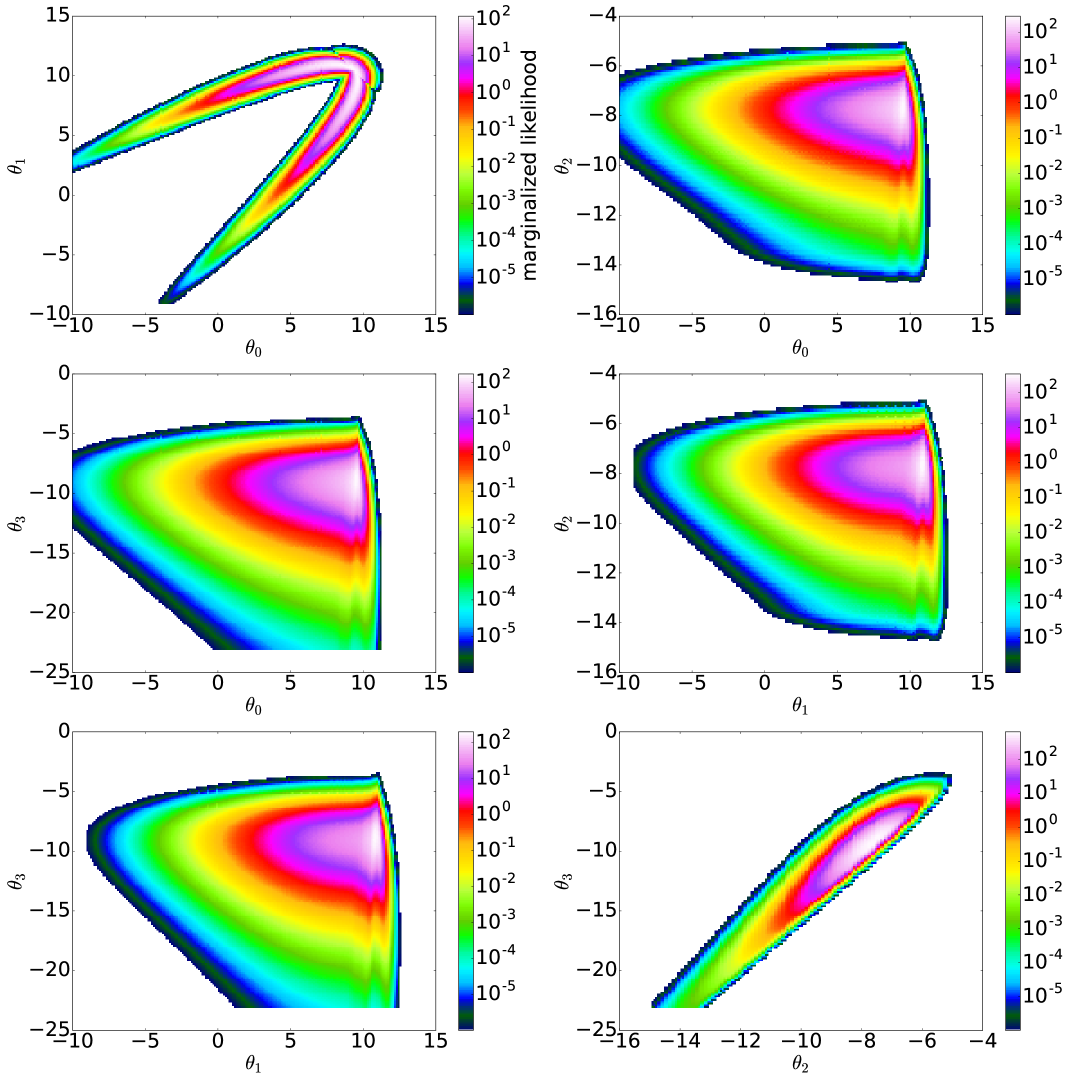
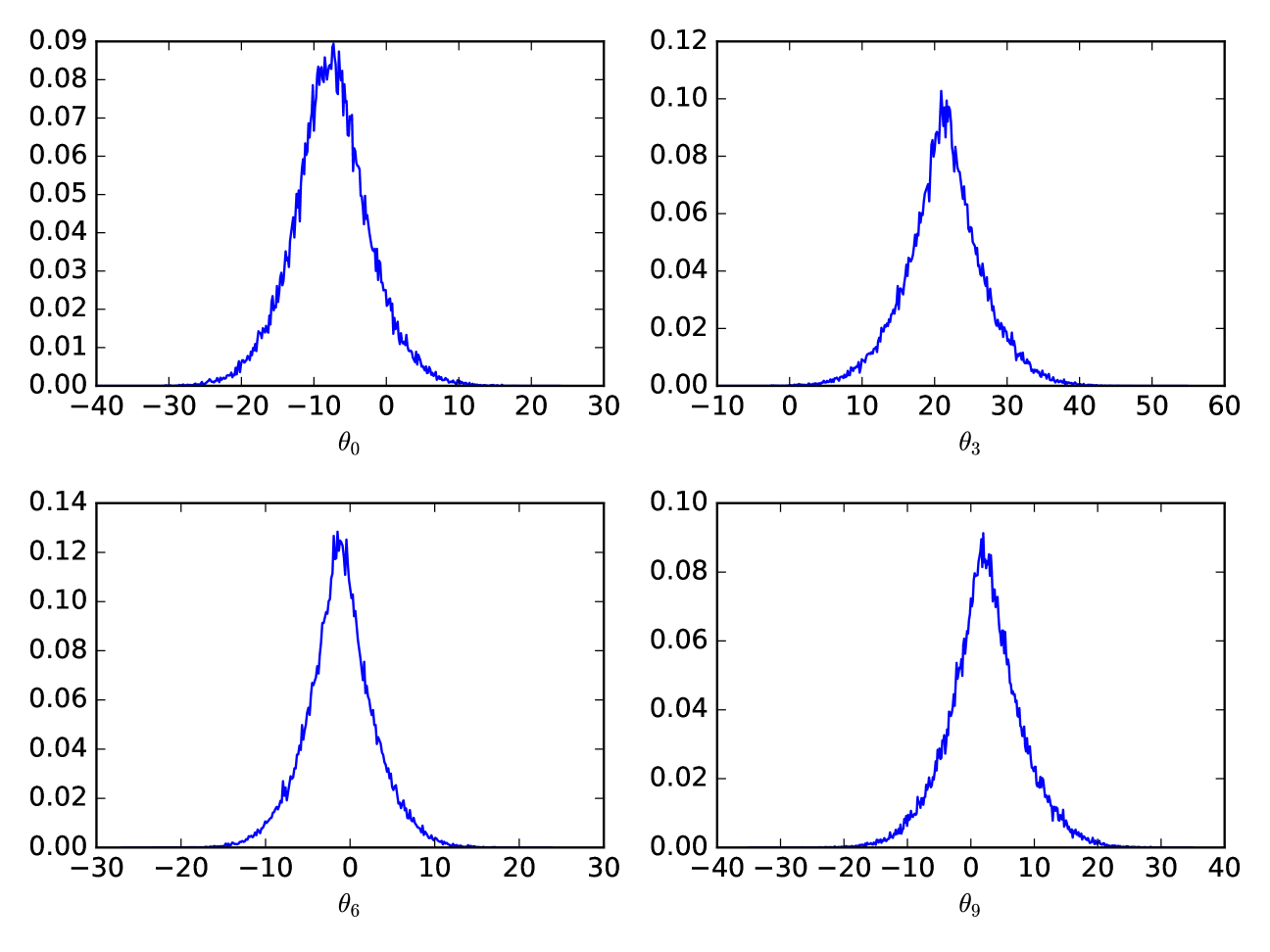
In order to compare different definitions of confidence and credible limits, we construct a cartoon likelihood function on 4 parameters. Choosing such a low-dimensional parameter space allows us to grid the full space and directly integrate the Bayesian credible limits without requiring unreasonable computational resources. Figure 1 shows the marginalized likelihood of our 4-dimensional cartoon likelihood function in each of the 2-dimensional parameter sub-spaces. As one can see, we have constructed our cartoon likelihood function to have a severely curved degeneracy in the parameter sub-space and significantly non-Gaussian contours in the other five sub-spaces.
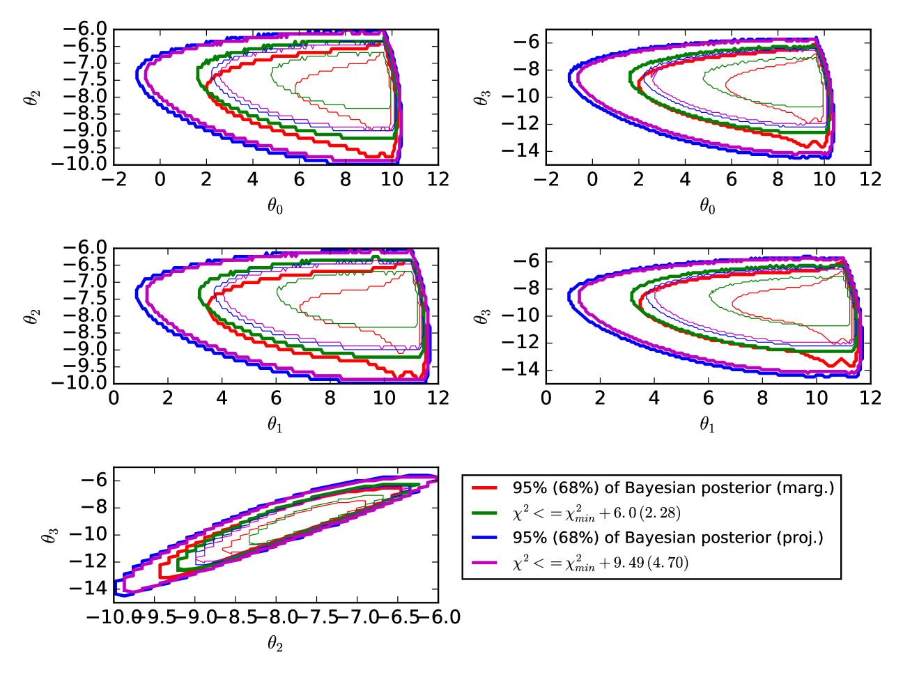
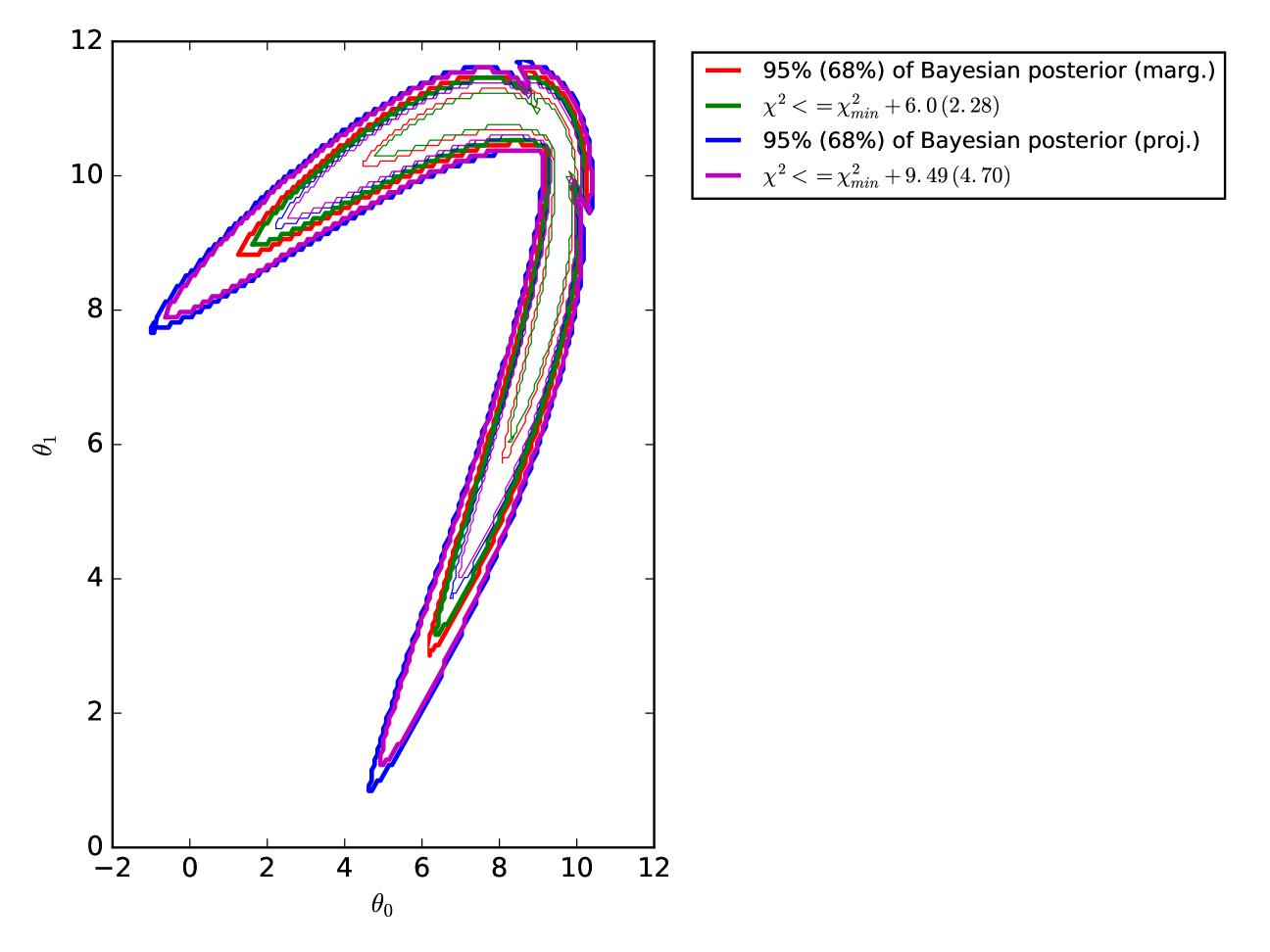
In Figures 2 and 3, we show the confidence and credible limits of our 4-dimensional toy likelihood function computed in several ways. The red contours show the marginalized Bayesian credible limits. These are the contours enclosing 95% (68%) of the marginalized likelihood shown in Figure 1. The green contours are the projections of the 4-dimensional contours enclosing , i.e. they were generated by finding all of the points in 4-dimensional space satisfying , converting those points into a scatter-plot in each of the 2-dimensional sub-spaces, and then drawing a contour around those scatter plots. Naively, one would expect these contours to be equivalent to the marginalized Bayesian contours, since 6.0 (2.28) is the 95% (68%) limit for a distribution with two degrees of freedom. (Note that the 95.4% and 68.3% limits, i.e. and in Gaussian probability, would have and 2.30.) This, however, is clearly not the case. The non-Gaussian nature of our toy likelihood prevents Wilks’ theorem from applying in the marginalized case. While you can integrate away dimensions of a -dimensional multivariate Gaussian and come up with a multivariate Gaussian, no such guarantee exists for arbitrary, non-Gaussian functions.
The blue contours in Figure 2 and 3 show the projected Bayesian credible limits of our cartoon function. These were constructed by assembling all of the points in 4-dimensional space that contained 95% (68%) of the total likelihood, converting those points to a scatter plot in the 2-dimensional sub-spaces, and drawing a contour around the scatter plots. The purple contours show the similarly projected contours containing all of the points for which , with 9.49 (4.70) being the 95% (68%) limit for a distribution with four degrees of freedom. We refer to these contours as the “full-dimensional LRT (likelihood ratio test)” contours. We see remarkably good agreement between the projected Bayesian and full-dimensional LRT contours in both the 95% and the 68% limit, in accordance with Wilks’ theorem (since we have not marginalized away any of the 4 parameters in our parameter space, Wilks’ theorem still appears to hold).
In the rest of this paper, we will examine likelihood functions based on their projected Bayesian and full-dimensional LRT contours. Though it is traditional to consider marginalized contours in 2-dimensional sub-spaces, we note concerns that this may discard important information about the actual extent of parameter space considered reasonable by the likelihood function. In all cases in Figures 2 and 3, the projected Bayesian and full-dimensional LRT contours were larger than their 2-dimensional marginalized counterparts. This should not be surprising. The projected Bayesian and full-dimensional LRT contours contain all of the pixels in the full 4-dimensional space that fall within the desired credible limit. The marginalized counterparts take those full 4-dimensional contours and then weight them by the amount of marginalized parameter space volume they contain. The final marginalized contour thus represents an amalgam of the raw likelihood function and its extent in parameter space. It is not obvious that this is necessarily what one wants when inferring parameter constraints from a data set.
If a point in parameter space falls within the projected Bayesian or full-dimensional LRT contour, it means that the fit to the data provided by that combination of parameters is, by some metric, reasonable. This is somewhat a matter of taste, but if one is really interested in all of the parameter combinations that give reasonable fits to the data, the conservative approach would be to keep all such combinations, rather than throwing out some, simply because they include rare – but fully accepted by the data – combinations of, say, (in the case of the gap between the marginalized and projected Bayesian contours in the plot in Figure 2). For this reason, we proceed111 We do not consider useful the strictly frequentist perspective that, since our cartoon likelihood function “measures” at 100 values of , the confidence limit limit should therefore be set according to the distribution with 100 degrees of freedom. This would set the 95% confidence limit at . Note that since for our toy likelihood function ended up being 83.12, such frequentist confidence limit contours would be significantly larger than anything shown in Figures 2 and 3. Such large contours seem unlikely to be useful. , comparing the performance of DALE with MultiNest by examining the projected Bayesian and full-dimensional LRT contours.
We acknowledge that there are some applications for which the approximate equivalence of with a Bayesian credible limit for which we have argued above is insufficient. If a likelihood function is sufficiently non-Gaussian or a data set is sufficiently noisy, the two will not be equivalent. Indeed, in Figures 2 and 3, the blue and purple contours are not identical, but merely approximately the same. In cases where only the Bayesian credible limit is acceptable, we still believe that there is a use for DALE . Bayesian sampling algorithms generally get bogged down during “burn-in”, the period of time at the beginning of the sampling run during which the algorithm is simply learning where the minimum point is and what the degeneracy directions of the contour are without efficiently sampling from the posterior. We show below that DALE converges to its confidence limits, with the same and degeneracy directions as the Bayesian credible limit, irrespective of one’s opinion of Bayesian versus frequentist statistical interpretations, after an order of magnitude fewer calls to than required by MultiNest. If one does not feel inclined to trust the full confidence limits returned by DALE , one should be able to achieve a significant speed-up in Bayesian sampling algorithms by using DALE as pre-burner: defining the region of parameter space to be sampled before sampling commences.
5 Comparison of Techniques
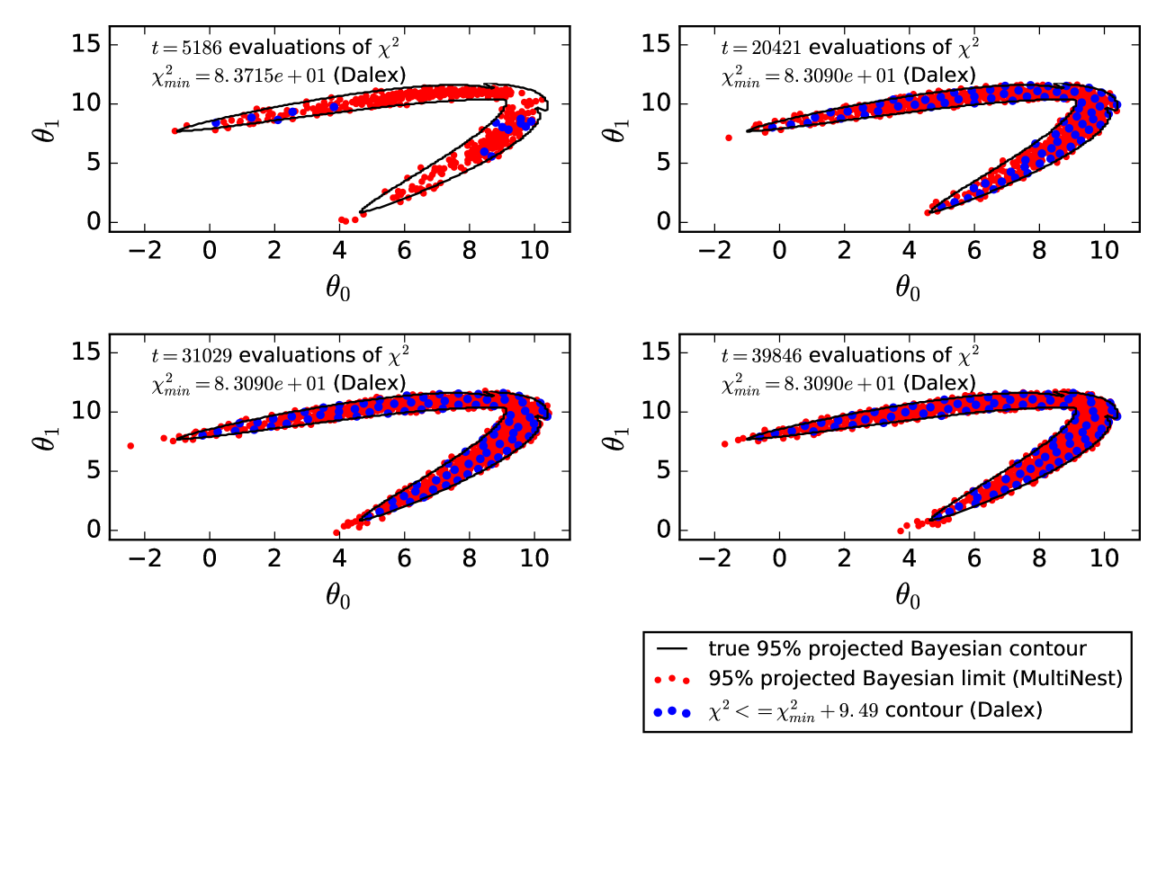
As a proof of concept, we begin by comparing the performance of MultiNest and DALE on the 4-dimensional likelihood function presented in Figure 1. As said before, four is an extremely low dimensionality and we find that MultiNest converges thoroughly and much more rapidly than DALE (though MultiNest does include some spurious points compared to exact, brute force calculation, unlike DALE , i.e. it has lower purity). Later, we will see that DALE out-performs MultiNest on higher-dimension likelihood functions. The purpose of this current discussion is to demonstrate that DALE does, in fact, find the limits expected from Figures 2 and 3.
Comparing MultiNest and DALE requires defining how long each should run. Because MultiNest is a sampling algorithm designed to integrate the posterior distribution, it has a well defined convergence criterion: when the Bayesian evidence integrated over parameter space ceases to grow, the sampling is done. DALE does not have any analogous global convergence criterion. Individual tendril searches within DALE can be said to converge when they “strike out” (see Section 3.2.4) but this says nothing about the overall convergence of DALE . It is up to the user to specify how many evaluations they wish DALE to make. In Figure 4 below, we wish to show the convergence of MultiNest and DALE as a function of “time” (time being measured in the number of evaluations being made). To do this, we initialized several MultiNest runs, each with a different number of “live” points. MultiNest instances with more live points took longer to converge (but can be expected to evaluate the posterior distribution more accurately). We then ran a single instance of DALE and asked it to quit after 40,000 evaluations. In Figure 4, we compare the MultiNest runs with the progress made by DALE after it had evaluated as many times as it took MultiNest to converge. The red points are the 2-dimensional projections of the points discovered by MultiNest to be in the 95% Bayesian credible limit. The blue points are the points discovered by DALE at the equivalent point in time. As stated, DALE does indeed find the correct contour while MultiNest is faster for and somewhat impure. We show below that, in higher-dimensional cases, DALE characterizes the contour much more robustly than MultiNest. We used version 3.9 of MultiNest here and throughout this paper. The most up-to-date version of MultiNest can be downloaded from https://ccpforge.cse.rl.ac.uk/gf/project/multinest/
5.1 Comparison on 12-dimensional case
We showed above that DALE found similar confidence limits, but took much longer to converge than did MultiNest on a 4-dimensional likelihood function. Now we compare DALE to MultiNest on a 12-dimensional cartoon likelihood function. Here we find that DALE converges an order of magnitude faster than MultiNest.
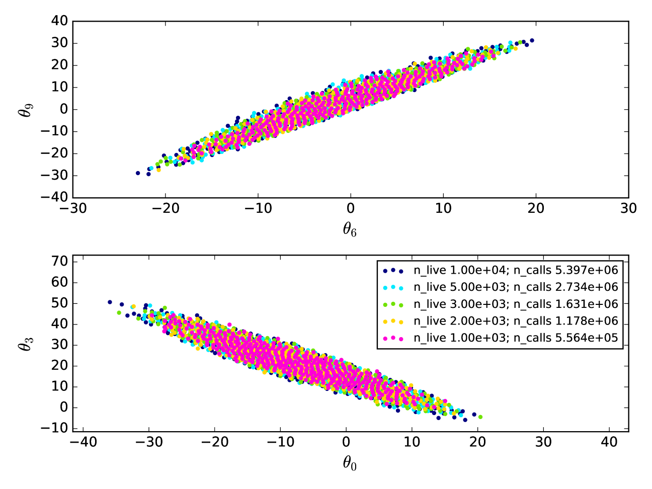
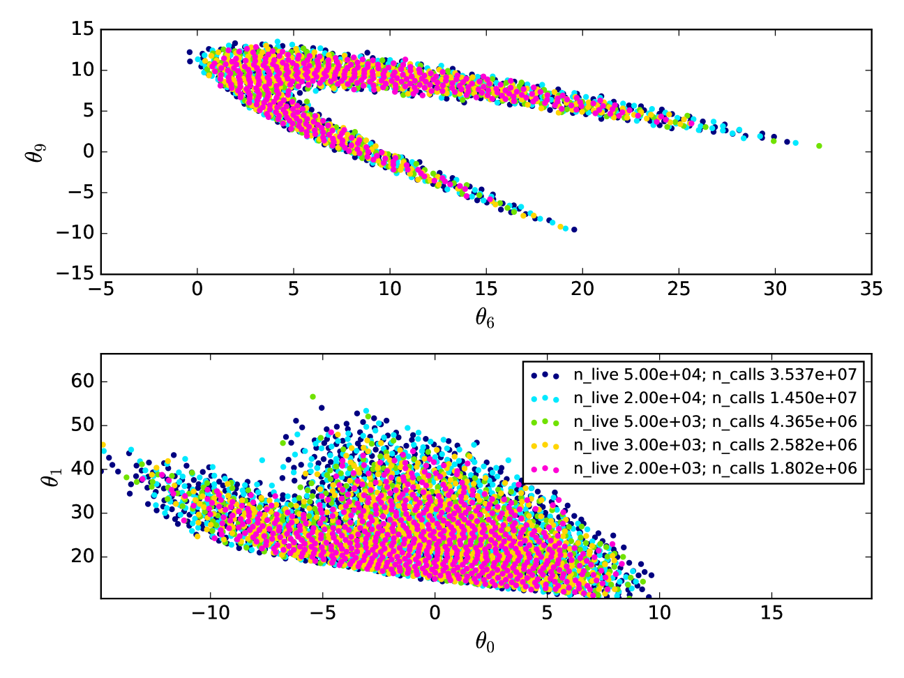
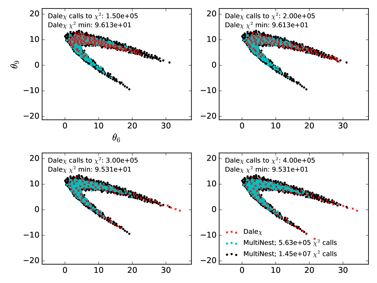
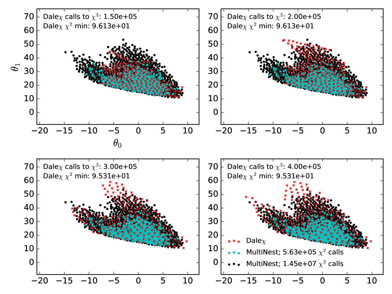
Before we show the direct comparison between DALE and MultiNest, we must be careful to define what we are comparing. MultiNest involves several user-determined parameters that control how the sampling is done. One in particular, the number of ‘live’ points, which is somewhat analogous to the number of independent chains run in an MCMC, has a profound effect both on how fast MultiNest converges and what limit it finds when it does converge. We created two 12-dimensional instantiations of our cartoon likelihood function, one with a very curved parameter space degeneracy, one without, and ran several instantiations of MultiNest with different numbers of ‘live’ points on those functions. Figures 5 and 6 show the projected Bayesian 95% credible limits found by MultiNest in two 2-dimensional sub-spaces for each of those likelihood functions as a function of the number of ‘live’ points. The figures also note how many evaluations of the likelihood function were necessary before MultiNest declared convergence. Not only does increasing the number of ‘live’ points increase the number of likelihood evaluations necessary for MultiNest to converge, it also expands the discovered credible limits. We interpret this to mean that running MultiNest with a small number of ‘live’ points results in convergence to an incomplete credible limit. When comparing DALE to MultiNest, we must therefore be careful which instantiation of MultiNest we compare against. Selecting a MultiNest run with too few ‘live’ points could mean that MultiNest appears as fast as DALE , but converges to an incorrect credible limit. Selecting a MultiNest run with too many ‘live’ points ensures that MultiNest has converged to the correct credible limit, but in an artificially large number of likelihood evaluations. In Figures 7 and 8, and Figures 10 and 11 below, we compare DALE both to a MultiNest instantiation that we believe has converged to the correct credible limit and a MultiNest instantiation that converges in a time comparable to DALE . This is to illustrate the relationship between convergence time and accuracy in MultiNest.
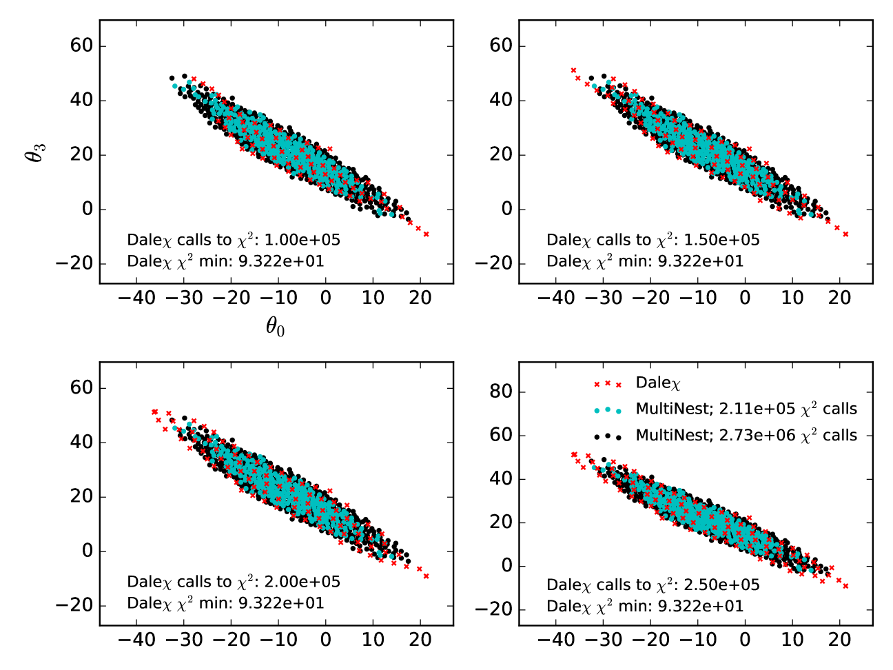
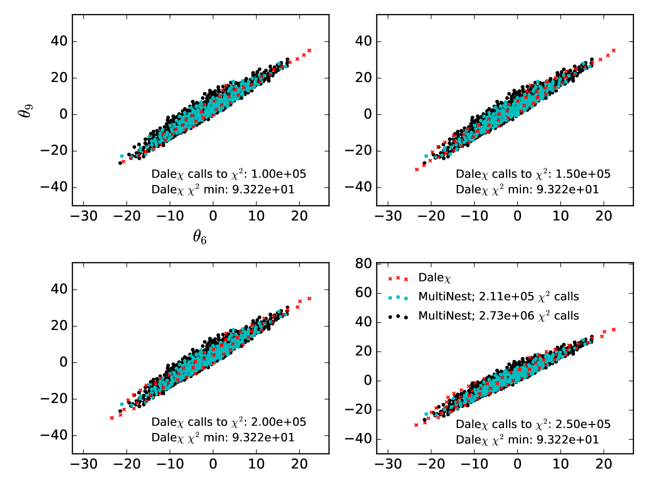
In Figures 7 and 8 we compare the convergence of DALE with that of MultiNest as a function of time. The likelihood function considered is a 12-dimensional cartoon constructed as in Section 4, but without the highly curved degeneracy direction. Each panel in the figures shows the state of the 95% confidence limits discovered by DALE after a specified number of evaluations of the likelihood function. The limits are plotted as scatter plots of the points discovered by DALE at that point in time. Because MultiNest does not produce chains in the same way that MCMC does, we cannot display the evolution of the credible limit found by MultiNest as a function of time. Instead, we plot two credible limits: one found by an instantiation of MultiNest that converges after evaluations of the likelihood function and one that converges after evaluations of the likelihood function. As explained above, this difference in convergence time was achieved by tuning the number of ‘live’ points in the MultiNest run. There are two important features to note here.
The first feature is that DALE has converged to its final credible limit after about 125,000-150,000 calls to . The second feature is the difference between the credible limits discovered by the two instantiations of MultiNest. True, one of the MultiNest instantiation converges in roughly (within a factor of two) as many likelihood evaluations as DALE . This instantiation of MultiNest, however, fails to explore the full non-Gaussian wings of the credible limit. See Figure 9 for a visualization of the non-Gaussianity. The slower MultiNest instantiation does find the same limits as DALE . However, it requires more than an order of magnitude more likelihood function evaluations to do so. This is the origin of our claim that DALE converges an order of magnitude faster than MultiNest on high-dimensional likelihood functions. DALE does not do as well as MultiNest characterizing the full width of the contour in the narrow degeneracy direction in Figure 8. However, by the end of the full 250,000 -evaluation run, one can see the wings of the contour beginning to trace out the full boundary. (Alternately, if one adopted the strategy suggested at the end of Section 4.1, using DALE to set the proposal distribution for a sampling algorithm, one could imagine filling in these contours more thoroughly than with just MultiNest alone while still only requiring 10% more evaluations of the likelihood function.)
Figures 10 and 11 show a similar comparison in the case of a 12-dimensional likelihood function with a highly curved parameter space degeneracy. Here again we see that DALE finds essentially the same limits as MultiNest, but more than an order of magnitude faster. We have done preliminary tests with a 16-dimensional likelihood function. These show almost two orders of magnitude speed-up of DALE vis-á-vis MultiNest. In the 16-dimensional case, MultiNest requires 75 million calls to to converge. DALE finds the same credible limit after only 1 million calls to .
Regarding some computational specifics, note we have been measuring the speed of DALE and MultiNest in terms of how many calls to are required to reach convergence. This is based on the assumption that, for any real physical use of these algorithms, the evaluation of will be the slowest part of the computation. For MultiNest, this is a fair assumption. As a Markovian process, the present behavior of MultiNest does not depend on its history. The same statement is not true of DALE . Because DALE is attempting to evaluate at parameter-space points as far as possible away from previous evaluations, DALE must always be aware of the full history of its search. Thus, the DALE algorithm implies some computational overhead in addition to the expense of simple evaluating . For our 12-dimensional test cases, this overhead averages out to between 0.005 and 0.015 seconds per evaluation on a personal laptop with a 2.9 GHz processor. For the 16-dimensional test case referenced above, this overhead varied between 0.01 and 0.03 seconds per evaluation on the same machine. It is possible that future work with an eye towards computational optimization could reduce these figures. It is also possible that the steady march of hardware innovation could render such concerns irrelevant going forward. The memory footprint of DALE appears to be well within the capabilities of modern personal computers.
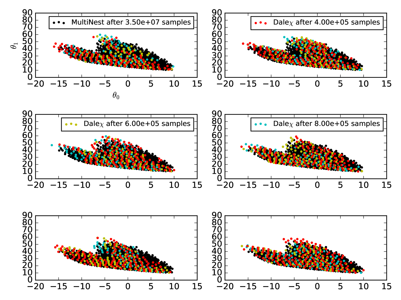
Note that both MultiNest and DALE depend on random number generators: MultiNest for driving sampling of the posterior, DALE for driving the Metropolis-Hastings-like algorithms described in Sections 3.1 and 3.2.2, and for selecting seeds for the simplex minimizations described in Sections 3.2.3 and 3.2.4. We have found that the convergence performance of DALE can depend on how that random number generator is seeded. Figure 12 plots six different runs of DALE , each with a different random number seed. The runs plotted were specifically selected to represent instances of DALE that did not find the full confidence limit after 400,000 evaluations (all six successfully found the confidence limit in 400,000 samples). In each panel, we show the confidence limit as found by DALE after 400,000, 600,000, 800,000 evaluations plotted against the true credible limit as discovered by a run of MultiNest with 50,000 live points, taking 35 million evaluations. In each case, the 400,000 evaluation confidence limit traces out the general shape of the true contour while the subsequent evaluations allow DALE to fill in the gaps in that first discovered confidence limit. Referring back to Figure 6, we see that, even after 4.3 million evaluations, MultiNest has not found its final credible limit. Therefore, even these instances of sub-optimal runs of DALE demonstrate a significant speed-up vis-à-vis MultiNest. The difficulty is in knowing how many evaluations is enough for DALE . This is the danger in not having a clear global convergence criterion for DALE and a subject worthy of further study.
For those interested, and in the interest of giving credit where credit is due, DALE uses the random number generator proposed by Marsaglia (2003) with initialization parameters proposed by Press et al. (2007). This is implemented in the class Ran defined in include/goto_tools.h in our code base.
5.2 Efficiency of Sampling
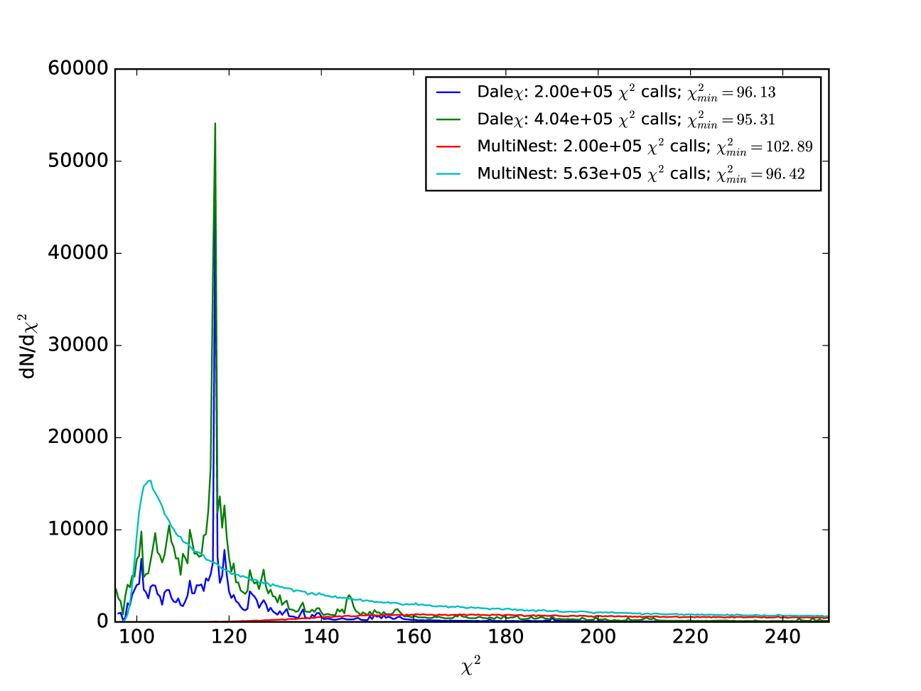
Figure 13 shows the distribution points evaluated by DALE and MultiNest as a function of when run on the highly curved likelihood function from Figures 6, 10, and 11. Note how DALE places a much larger fraction of its points on the contour than does MultiNest. This should not be surprising as DALE was designed with limit-finding in mind. MultiNest is a code designed to calculate the integrated Bayesian evidence of a model. The fact that one can draw confidence limit contours from the samples produced by MultiNest is basically a happy side-effect of this evidence integration. Because it focuses on finding the contours directly, rather than integrating the posterior over parameter space, DALE is highly efficient at both the optimization and characterization tasks, i.e. the key elements of determining the best fit and its error estimation, as designed. This tradeoff between obtaining the two critical elements for parameter estimation versus mapping the posterior more broadly (and sometimes less accurately) is the root cause of the vastly improved speed demonstrated by DALE .
6 Conclusions
As our exploration of the universe becomes increasingly detailed and precise, the range of astrophysical, instrumental, and theoretical systematics that must be taken into account require high dimensional parameter spaces. Accurate estimation of the desired parameters needs fast and robust techniques for exploring high dimensional, frequently nonlinearly degenerate and non-Gaussian joint probability distributions. DALE is designed with two paramount purposes: optimization – finding the probability maximum, and characterization – mapping out a specified confidence limit .
We have shown that its blend of strategies: to obtain robustly the maximum, search for multiple maxima, focus on the desired confidence limit, and efficiently map it out along multiple dimensions by seeking points distinct from established points and tracing along curved degeneracies – can be quite successful. This diversity is important in cases where the likelihood is not known to be close to Gaussian but may have complicated, degenerate/highly curved/non-Gaussian, or multimodal properties. DALE exhibits excellent completeness and purity: it routinely finds viable regions of the posterior missed by Markov Chain Monte Carlo or MultiNest nested sampling, and it focuses its search in the critical areas rather than accreting points not directly relevant to the maximum or confidence limit.
In the low, four dimensional test case, DALE had better purity (i.e. accuracy of confidence limit estimation) but MultiNest was faster. By the more common case of a 12 dimensional parameter space, DALE achieve a speed advantage of nearly a factor of 10. Note that DALE looks for a user specified confidence limit, e.g. 95%; if the user wants multiple confidence limits, e.g. also 68%, then it is true that DALE must be rerun while MultiNest can generate it from its original results. However, the factor 10 speed advantage (coupled with that the first run of DALE will have already completed the optimization step of finding the probability maximum), means that even for calculation of several confidence limits the speed advantage remains. With higher dimensional parameter spaces we expect the advantage to become even stronger (unless the likelihood function is close to Gaussian in all dimensions). A preliminary test on a 16-dimensional likelihood function showed a factor of 75 speed advantage to DALE over MultiNest. At a minimum, DALE can function as a highly efficient “pre-burner” for sampling methods.
Despite its current success, several areas remain open for further improvement to DALE . It seems likely that the refinement procedure could be improved in efficiency. The convergence criterion is local and somewhat heuristic; potentially a more robust condition could further improve performance. Note that DALE is open source so we encourage interested researchers to explore its use and join in to make it even better. It serves as a new tool in our quest to estimate accurately the parameters of our universe.
The Direct Analysis of Limits via the Exterior of (DALE ) has as its mission to look for the terminus of the desired confidence region, the boundary separating it from the unfavored exterior parameter space. One could say that in its quest to keep only the viable models, by terminating the exterior, the watchword for DALE is ex-terminate. Finally, DALE is available at https://github.com/danielsf/Dalex.git .
Appendix A Fitting ellipsoids to samples
In order to prevent DALE from wasting time exploring regions of parameter space that have already been discovered, we require a construct that represents the region in parameter space bounded by a set of sampled points in such a way that we can quickly determine whether a new point is inside (in which case, DALE is doubling back on itself and must be corrected) or outside (in which case, DALE has discovered a new region of ) that region. The simplest way to represent such a region would be to construct a hyperbox whose edges are at the extremal values of each cardinal dimension as described by the points in . This, however, would involve erroneously designating too much unexplored volume as “explored”. Consider the case where the samples in are tightly clustered around the diagonal of a three-dimensional cube. Using the extremal values of in would entail designating the entire cube as “explored” when, in fact, we know almost nothing about the cube as a whole. We therefore have implemented the following algorithm to take the set of sampled points and determine a nearly volumetrically minimal ellipsoid containing . This is the region that we designate as “explored” for the purposes of DALE .
The first step in designating our ellipsoid is to find the center of the ellipsoid. To do this, we find the extremal values of in the cardinal dimensions ( in a three-dimensional example). We determine the geometric center of to be at the point
| (A1) |
where is an index over the dimensions of parameter space. We set the center of our ellipsoid to be the point in that is closest to where, for the purposes of this determination, we calculate the distance to be
| (A2) |
Note the dimensions in parameter space are normalized by the denominator so each dimension runs from 0 to 1, putting them on an equal footing.
Once we have found the center of our ellipsoid, which we call , we must find the basis directions along which the axes of our ellipsoid will be reckoned. Initialize an empty set of -dimensional vectors . Iterate over the points in . For each point, calculate the vector
| (A3) |
where are the orthogonal unit vectors already in . Select the vector with the largest L2 norm. Normalize this vector and add it to . Continue until there are vectors in . In this way, we select a set of orthogonal basis vectors along which the points are extremally distributed.
Now that we have determined the center and bases of the coordinate system in which we will draw our ellipsoid, we must find a set of lengths of the ellipsoid’s axes such that all of the points in are contained in the ellipsoid. The length of the vectors chosen to populate provide a good first guess at this set of lengths, but they are only guaranteed to describe the ellipsoid if the points in really are only distributed along the vectors and centered on . Since this seems unlikely, we adopt an iterative scheme to adjust the lengths so that our ellipsoid contains . For each of the points that are not contained by the ellipsoid, find the basis vector that maximizes
| (A4) |
where is the length in corresponding to that basis vector. Keep track of the number of points for which any given basis vector is . Select the basis direction that is for the most points . Multiply the corresponding by 1.1. Continue this process until there are no more points .
This algorithm is implemented in include/ellipse.h and src/utils/ellipse.cpp in our code base.
References
- Bentley (1975) Bentley, J. L. 1975, Communications of the Association for Computing Machinery 18, 509
- Brooks and Gelman (1998) Brooks, S. and Gelman A. 1998, Journal of Computational and Graphical Statistics 7, 434
- Bryan (2007) Bryan, B., 2007, Ph.D. thesis, Carnegie Mellon University, http://reports-archive.adm.cs.cmu.edu/anon/ml2007/abstracts/07-122.html
- Bryan et al. (2007) Bryan, B., Schneider, J., Miller, C. J., Nichol, R. C., Genovese, C., and Wasserman, L., 2007, Astrophys. J. 665, 25
- Casella and George (1992) Casella, G. and George, E. I. 1992, The American Statistician 46, 167
- Daniel et al. (2014) Daniel, S.F., Connolly, A.J., and Schneider, J. 2014, ApJ 794 38 [arXiv:1205.2708]
- Feroz and Hobson (2008) Feroz, F. and Hobson, M.P. 2008, Monthly Notices of the Royal Astronomical Society 384, 449
- Feroz et al. (2009) Feroz, F., and Hobson, M. P., and Bridges, M. 2009, Monthly Notices of the Royal Astronomical Society 398, 1601
- Feroz et al. (2013) Feroz, F., Hobson, M. P., Cameron, E., and Pettitt, A. N., arXiv:1306.2144
- Gelman and Rubin (1992) Gelman, A. and Rubin, D. 1992, Statistical Science 7, 457
- Kirkpatrick et al. (1983) Kirkpatrick, S., Gelatt, C. D., and Vecchi, M. P. 1983, Science 220, 671
- Marsaglia (2003) Marsaglia, G. 2003, Journal of Statistical Software, 8 14
- Nelder and Mead (1965) Nelder, J. A. and Mead, R. 1965, The Computer Journal, 7 308
- Planck Collaboration (2013) Planck Collaboration XVI 2014, Astronomy & Astrophysics 571 16 [arXiv:1303.5076]
- Press et al. (2007) Press, W. H., Teukolsky, S. A., Vetterling, W. T. and Flannery, B. P. 2007, “Numerical Recipes” (3d edition), Cambridge University Press, 2007
- Rasmussen and Williams (2006) Rasmussen, C. E. and Williams, C. K. I., 2006, “Processes for Machine Learning” http://www.GaussianProcess.org/gpml
- Skilling (2004) Skilling J. 2004, in “Bayesian Inference and Maximum Entropy Methods in Science and Engineering”, eds. Fisches R., Preuss R., von Toussaint U., AIP Conf. Proc. 735, 395
- Wilks (1938) Wilks, S. S. 1938, Annals of Mathematical Statistics, 9 60