Acceleration by Random Stepsizes:
Hedging, Equalization, and the Arcsine Stepsize Schedule
Abstract
We show that for separable convex optimization, random stepsizes fully accelerate Gradient Descent. Specifically, using inverse stepsizes i.i.d. from the Arcsine distribution improves the iteration complexity from to , where is the condition number. No momentum or other algorithmic modifications are required. This result is incomparable to the (deterministic) Silver Stepsize Schedule which does not require separability but only achieves partial acceleration . Our starting point is a conceptual connection to potential theory: the variational characterization for the distribution of stepsizes with fastest convergence rate mirrors the variational characterization for the distribution of charged particles with minimal logarithmic potential energy. The Arcsine distribution solves both variational characterizations due to a remarkable “equalization property” which in the physical context amounts to a constant potential over space, and in the optimization context amounts to an identical convergence rate over all quadratic functions. A key technical insight is that martingale arguments extend this phenomenon to all separable convex functions. We interpret this equalization as an extreme form of hedging: by using this random distribution over stepsizes, Gradient Descent converges at exactly the same rate for all functions in the function class.
1 Introduction
It is classically known that by using certain deterministic stepsize schedules , the Gradient Descent algorithm (GD)
| (1.1) |
solves convex optimization problems to arbitrary precision from an arbitrary initialization . This result can be found in any textbook on convex optimization, e.g., [9, 10, 40, 45, 30, 38, 6, 35]. The present paper investigates the following question:
| Is it possible to accelerate the convergence of GD by using random stepsizes? | (1.2) |
In this paper, we show that for separable convex optimization, the answer is yes. Specifically, we provide an i.i.d. stepsize schedule that makes GD converge at the optimal accelerated rate. See §1.1 for a precise statement; here we first contextualize with the relevant literature on random stepsizes.
Note that the use of randomness for GD stepsizes is conceptually different from the standard use of randomness in Stochastic Gradient Descent (SGD). SGD has random, inexact gradient queries and typically use deterministic stepsizes. GD has exact gradient queries, and random stepsizes amounts to purposely injecting noise into the algorithm.
The special case of quadratics.
This question is understood (only) for optimizing convex quadratic functions. In particular, the line of work [47, 63, 32] shows that for quadratic functions that are -strongly convex and -smooth (i.e., ), there is a unique optimal distribution for i.i.d. stepsizes that makes GD converge at a rate of
| (1.3) |
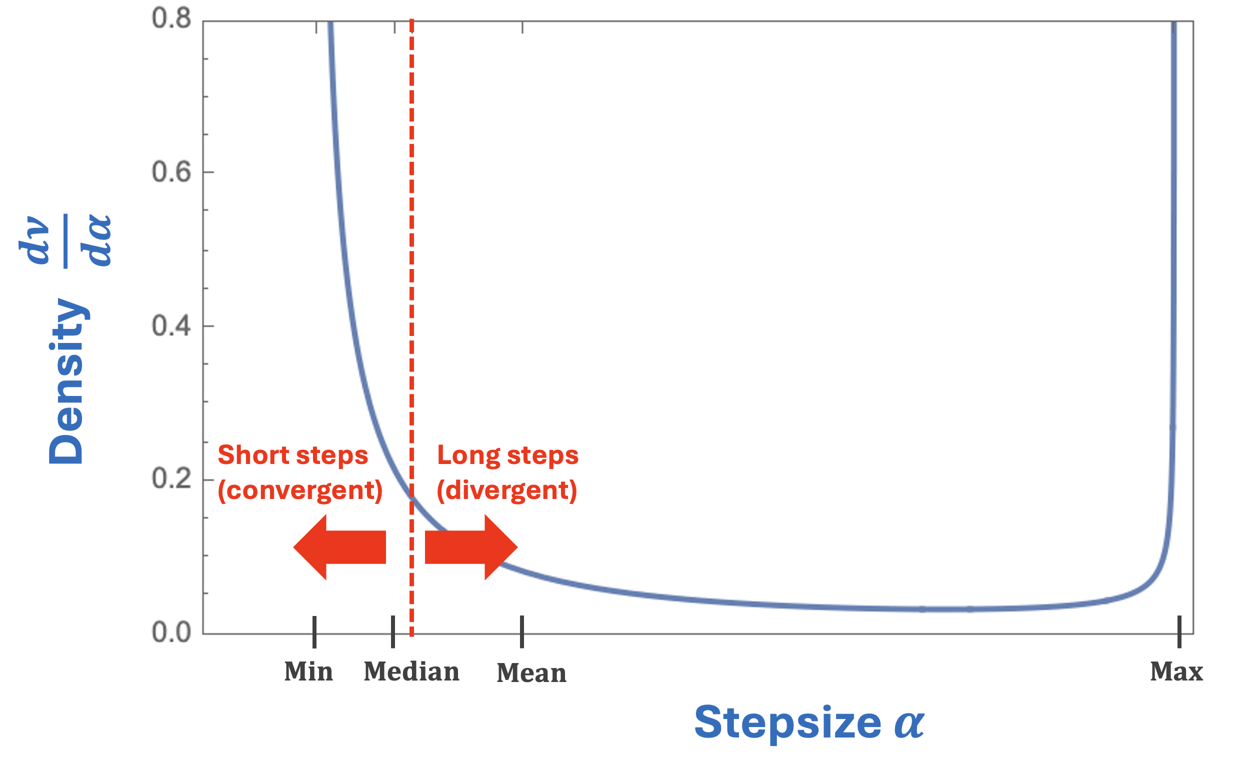
where denotes the minimizer of , denotes the condition number, and this convergence is in an appropriate probabilistic sense (e.g., almost-sure or ). This stepsize distribution is most naturally stated in terms of the inverse stepsizes having the Arcsine distribution on the interval , i.e., density
| (1.4) |
Briefly, this Arcsine distribution arises naturally for the special case of quadratics because: (1) the convergence rate is invariant w.r.t. the stepsize order and thus depends only on the empirical measure of the stepsizes; and (2) the Arcsine distribution is the limit as of the empirical measure of the optimal (deterministic) stepsizes for GD [61]. See §2.1 for details.
The resulting convergence rate (1.3) requires roughly iterations to produce an -accurate solution. Such a rate is called “accelerated” because its dependence on improves over the standard iteration complexity required by GD with constant stepsizes. Moreover, this convergence rate is information-theoretically optimal for any first-order algorithm [40, 39], and matches the worst-case convergence rate of accelerated algorithms that change GD beyond just its stepsizes, e.g., the Conjugate Gradient method [31], Polyak’s Heavy Ball method [44], Nesterov-style momentum methods [41], and more [22]. See Table 1, left.
Beyond quadratics?
For general convex optimization, momentum-based algorithms still achieve these optimally accelerated rates . However, existing acceleration results for random stepsizes do not extend beyond the special case of quadratic functions —otherwise is non-linear, making GD a non-linear map, which completely breaks all previous analyses. This failure of the analyses is due to fundamental differences between quadratic optimization and convex optimization:
- •
-
•
The convergence rate is invariant w.r.t. the stepsize order for quadratic optimization (which motivates the opportunity for random stepsizes), but this is false for convex optimization [2].
-
•
Using time-varying stepsizes is equivalent to using momentum for quadratic optimization (which enables GD to achieve accelerated rates), but this is false for convex optimization [22].
Due to these challenges, it remained unclear whether random stepsizes could lead to the accelerated rate for convex optimization. In fact, it was unknown even if random stepsizes could provide an arbitrary small improvement over the rate of constant-stepsize GD in any setting beyond quadratic optimization.
1.1 Contribution and discussion
This paper shows that random stepsizes provably accelerate GD beyond the setting of quadratics. Specifically, our main result (Theorem 1.2) shows that GD converges at the optimally accelerated rate for separable convex functions. This separability property is defined below and, for functions , is equivalent to commutativity of the Hessians , see Appendix B.1.
Definition 1.1 (Separable functions).
A function is separable if it admits a decomposition of the form
| (1.5) |
for some orthogonal matrix and some functions .
Theorem 1.2 (Random stepsizes accelerate GD for separable convex optimization).
Consider any dimension , any separable function that is -strongly convex and -smooth, and any initialization point that is not equal to the minimizer of . By using i.i.d. inverse stepsizes from the Arcsine distribution (1.4), GD converges at the rate
| (1.6) |
where this convergence in the almost sure and sense. Moreover, this is the unique distribution for which GD achieves this optimal rate.
| Stepsizes \ Function class | Quadratic | Separable | Convex |
|---|---|---|---|
| Constant | folklore | folklore | folklore |
| Deterministic (Chebyshev/Silver) | [61] | [3] | [3] |
| Random (Arcsine) | [32, 47, 63] | Theorem 1.2 | unknown if randomness helps |
We make several remarks about this result.
Optimality.
Comparison to GD with different stepsize schedules.
Theorem 1.2 first appeared as Theorem 6.1 of the 2018 MS thesis [2] of the first author (advised by the second author). This was the first convergence rate for any stepsize schedule (deterministic or randomized) that improved over the textbook rate for constant-stepsize GD, in any setting beyond quadratics. Indeed, even though many stepsize schedules have been investigated in both theory and practice, none of these alternative schedules had led to an analysis that outperforms (even by an arbitrarily small amount) the “unaccelerated” contraction factor of constant stepsize GD, which corresponds to an iteration complexity of . This comparison statement includes even adaptive stepsize schedules such as exact line search [42, 9, 45, 15], Armijo-Goldstein schedules [40], Polyak-type schedules [45], and Barzilai-Borwein-type schedules [5]. Some of these schedules fail to accelerate even on quadratics (and therefore also on separable convex problems), a classic example being exact line search [33, §3.2.2].
In the years since [2], a line of work has shown partially accelerated convergence rates for general convex optimization using deterministic stepsize schedules [2, 12, 23, 13, 26, 3, 4, 27, 28, 58, 62, 29, 8]. In particular, [3] showed the Silver Convergence Rate for minimizing -conditioned functions by using a certain fractal-like deterministic stepsize schedule called the Silver Stepsize Schedule. This rate is conjecturally optimal among all possible deterministic stepsize schedules [3] and naturally extends to non-strongly convex optimization [4]. Theorem 1.2 is incomparable: it shows a fully accelerated rate , but under the additional assumption of separability. This incomparability raises several interesting questions about the possible benefit of randomization for GD. The future work section §7 collects several such conjectures.
Comparison to arbitrary first-order algorithms.
Starting from the seminal work of Nesterov in 1983 [41], the traditional approach for obtaining accelerated convergence rates is to modify the GD algorithm beyond just changing stepsizes, for example by adding momentum, extra state, or other internal dynamics. These results hold for arbitrary convex optimization and do not require separability. See for example [11, 21, 52, 56] for some recent such algorithms, and see the recent survey [22] for a comprehensive account of this extensive line of work. The purpose of this paper is to investigate an alternative mechanism for acceleration: can GD be accelerated in its original form, by just choosing random stepsizes?
Generality.
The assumptions in Theorem 1.2 can be relaxed. Separability can be generalized to radial-separability, and strong convexity and smoothness can be relaxed to less stringent assumptions on the spectrum of the Hessian of ; see §4 for details. Note also that since GD does not depend on the choice of the basis in the separable decomposition (1.5), Theorem 1.2 only requires the existence of some such (which is the definition of separability). In particular, the algorithm does not need to know . Also, Theorem 1.2 is stated for convergence in terms of distance to optimality, but extends to all standard desiderata; see §4. Theorem 1.2 also extends to settings where gradient descent is performed inexactly, e.g., due to using inexact gradients; see §6.1.
Opportunities for randomized stepsizes.
Randomized algorithms have variability in their trajectories. This provides potential opportunities for running multiple times in parallel and selecting the best run, see §5.3. This best run can be significantly better than the typical run (whose rate converges almost surely to the accelerated rate, see §5.2) and the worst run (whose rate can diverge but only with exponentially small probability, see §5.1).
Game-theoretic connections and lower bounds.
This paper considers random stepsizes in order to accelerate GD. This randomized perspective is also helpful for the dual problem of constructing lower bounds, i.e., exhibiting functions for which gradient descent converges slowly. In particular, lifting to distributions over functions leads to a game between an algorithm (who chooses a distribution over stepsizes) and an adversary (who chooses a distribution over functions) which is symmetric in that the Arcsine distribution is the optimal answer for both. This leads to new perspectives on classical lower bounds for GD; details in §6.2.
Techniques and connections to logarithmic potential theory.
A distinguishing feature of our analysis is a connection to potential theory: the variational characterization for the optimal stepsize distribution mirrors the variational characterization for a certain equilibrium distribution which configures a unit of charged particles so as to minimize the logarithmic potential energy. The optimal distribution satisfies a remarkable “equalization property” which in the physical context amounts to a constant potential over space, and in the optimization context amounts to an identical convergence rate over all quadratic functions. A key technical insight is that martingale arguments extend this phenomenon to all separable convex functions. While links between Krylov-subspace algorithms and potential theory are classical (see the excellent survey [19]), these connections are restricted to the special case of quadratics and moreover, even for that setting, these connections have not been exploited for the analysis of GD with random stepsizes. See §2 for a conceptual overview of our analysis techniques and how we exploit this equalization property to prove Theorem 1.2.
1.2 Organization
§2 provides a conceptual overview of our analysis approach. §3 proves our main result, Theorem 1.2. §4 discusses generalizations beyond separability, strong convexity, and smoothness. §5 investigates the variability from using randomized stepsizes, in terms of notions of convergence, high probability bounds, and opportunities for parallelized optimization. §6 provides auxiliary results about stability and game-theoretic interpretations. §7 describes several directions for future work that are motivated by our results. For brevity, several proofs are deferred to the appendix.
2 Conceptual overview: acceleration by random stepsizes
Here we provide informal derivations of our main result in order to overview the key conceptual ideas. We begin by briefly recalling in §2.1 how random stepsizes can accelerate GD for the special case of quadratic optimization. Then in §2.2, we describe the challenges for acceleration beyond quadratics, and our new techniques for circumventing these challenges.
2.1 Quadratic optimization
Consider running GD on the class of quadratic functions that are -strongly convex and -smooth. What is the optimal distribution from which to draw i.i.d. stepsizes? In order to understand this, we first recall the optimal deterministic stepsizes.
Optimal deterministic stepsizes.
Without loss of generality after translating,
| (2.1) |
Since the function is quadratic, its gradient is linear , hence GD is a linear map
| (2.2) |
and therefore the final iterate is
| (2.3) |
The convergence rate for a given stepsize schedule—in the worst case over objectives functions in and initializations —is therefore
| (2.4) | ||||
| (2.5) |
Above, the penultimate step is by definition of the spectral norm, and the final step is by diagonalizing. It is a simple and celebrated fact, dating back to Young in 1953 [61], that minimizing this convergence rate (2.5) over stepsizes is equivalent to a certain extremal polynomial problem, and that as a consequence, the optimal stepsizes minimizing (2.5) are the inverses of the roots of a (translated and scaled) Chebyshev polynomial, in any order. Said more precisely: for any horizon length , the optimal stepsizes are any permutation of
| (2.6) |
and the corresponding -step convergence rate in (2.5) is
| (2.7) |
Optimal random stepsizes.
Much less well-known is the fact that this accelerated rate can also be asymptotically achieved by simply using i.i.d. stepsizes from an appropriate distribution [32, 47, 63]. The intuition is that the convergence rate (2.5) is invariant in the order of the stepsizes, instead depending only on their empirical measure, and as one can achieve the same empirical measure (and thus the same convergence rate) by replacing the carefully chosen deterministic Chebyshev stepsize schedule (2.6) with i.i.d. stepsizes from their limiting empirical measure. See [2, Chapter 3] for a discussion of this through the lens of exchangeability and De Finetti’s Theorem.
Concretely, if the inverse stepsizes are i.i.d. from some distribution , then (forgoing measure-theoretic technicalities) the Law of Large Numbers ensures that the -step convergence rate in (2.5) converges almost surely and in expectation to
| (2.8) |
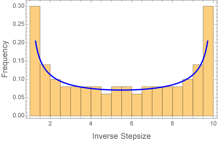
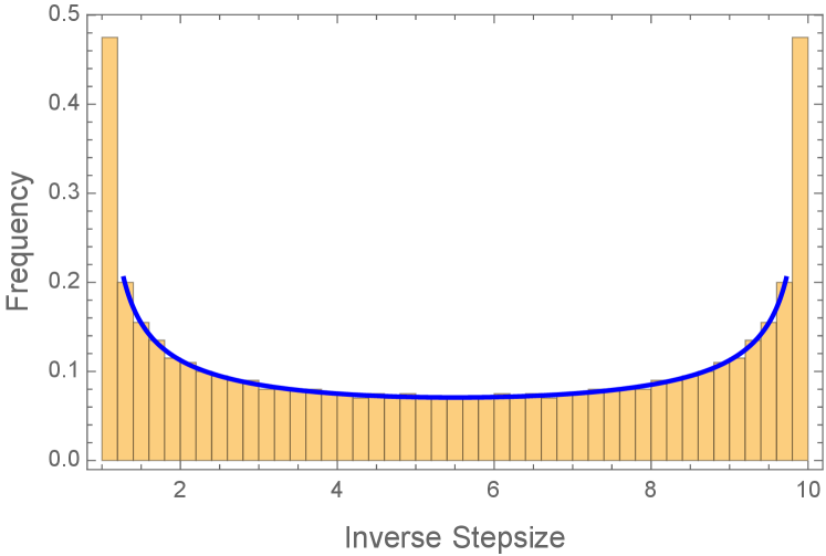
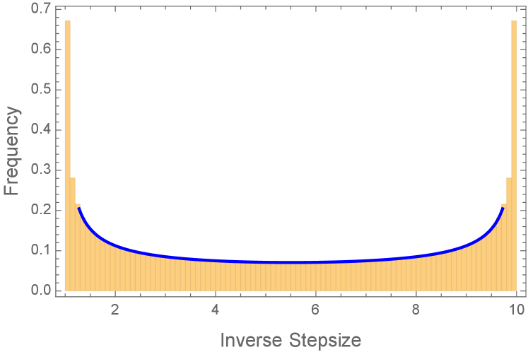
This informal derivation suggests that the distribution minimizing the asymptotic convergence rate (2.8) should be the appropriate limit as of the empirical measure for the inverse Chebyshev stepsize schedule (this limit is the distribution, since has the Arcsine distribution on if is uniformly distributed on see Figure 2), and moreover the optimal value should be the accelerated rate . This intuition is formalized by the following lemma.
Lemma 2.1 (Extremal property of the Arcsine distribution).
The extremal problem
| (2.9) |
has optimal value , achieved by the unique optimal solution .
This lemma was proven in the optimization literature via a long, tour-de-force integral calculation [32]. In Appendix A, we present an alternative, short proof from Altschuler’s thesis [2] that argues by connecting this extremal problem for stepsize distributions to a classical extremal problem in potential theory about electrostatic capacitors. The key feature of this connection is the following equalization property of the Arcsine distribution.
Lemma 2.2 (Equalization property of the Arcsine distribution).
For all ,
| (2.10) |
In particular, this value does not depend on .
This equalization property uniquely defines the Arcsine distribution in that there is no other distribution satisfying (2.10); see Appendix A. In words, this property shows that the Arcsine distribution “equalizes” the convergence rate over all quadratic functions (parameterized by their curvatures ). We emphasize that this is not just an algebraic identity: this equalization property also has a natural interpretation in terms of a game between an optimization algorithm (who chooses a stepsize to minimize the convergence rate) and an adversary (who chooses a quadratic function to maximize the convergence rate), see §6.2. In Appendix A we elaborate on the connections to potential theory, and leverage that connection to provide short proofs of these lemmas.
2.2 Beyond quadratic optimization
We now turn to accelerating GD beyond the special case of quadratic functions . The central challenge is that the curvature, as measured by the Hessian , is no longer constant. This breaks the above quadratic analysis in several ways since it is no longer possible to summarize or re-parameterize the Hessians along the GD trajectory in terms of a single scalar . To explain these issues, let us attempt to adapt this analysis to the general convex setting, assuming for simplicity here that is twice differentiable (our actual analysis in §3 avoids any such assumption).
Time-varying curvature.
Clearly, if is not quadratic, then the gradient is not linear, and as a consequence the GD map is not linear. Assuming as before that without loss of generality, one can generalize the linear GD map (2.3) to the non-quadratic setting as
| (2.11) |
since by the Fundamental Theorem of Calculus, and thus . The interpretation of is that it is the average Hessian between and , i.e., it measures the relevant local curvature in the -th iteration of GD. In the quadratic setting, for all since the Hessian is constant, which recovers (2.3) from (2.11). However, for the general non-quadratic setting, the curvature varies in . This is the overarching challenge mentioned above. For the purpose of accelerating GD, this challenge manifests in two interrelated ways: the lack of commutativity and predictability of the curvature along the trajectory of GD. Below we describe both challenges and how we circumvent them.
2.2.1 Issue 1: commutativity (deriving the extremal problem)
The first issue is that for convex functions, the Hessians at different points do not necessarily commute. Thus, in general, do not commute and therefore are not simultaneously diagonalizable. This precludes the key step (2.5) in the quadratic analysis above, which decomposes the convergence rate across eigendirections, thereby reducing the (multivariate) problem of convergence analysis to an analytically tractable (univariate) extremal problem. This is the only reason we assume separability: it is equivalent to commuting Hessians (Lemma B.1). Concretely, separability allows us to show an analog of (2.5) in which the convergence rate of a stepsize schedule is bounded by
| (2.12) |
the difference to the quadratic case being that there all are the same, whereas now can be time-varying and can depend on all previous stepsizes .
By taking an appropriate111A subtle but important technical issue is that one cannot simply use the Law of Large Numbers to derive the asymptotic convergence rate from the -step rate (c.f., (2.8) for how that worked in the quadratic case). Indeed, in the convex case here, the relevant empirical sum has non-i.i.d. summands: they are neither identically distributed (since is time-varying) nor independent (since can depend on previous stepsizes). Briefly, we overcome the identically distributed issue by using the equalization property of the Arcsine distribution (Lemma 2.2) to show that these summands still have the desired expectation, and we overcome the independence issue by using a martingale-based argument to show that the fresh randomness in makes these summands “independent enough” to prove a specially tailored version of Kolmogorov’s Strong Law of Large Numbers for this setting. Details in §3.1. limit of the -step convergence rate (2.12), it can be shown that the (logarithm of the) asymptotic rate for i.i.d. inverse stepsizes from a distribution is governed by the extremal problem:
| (2.13) |
where denotes the natural filtration corresponding to the inverse stepsizes . Observe that (2.13) recovers the extremal problem (2.8) for the quadratic case if are constant, but in general is different because can be time-varying. This brings us to the second issue.
2.2.2 Issue 2: unpredictability (solving the extremal problem)
The second issue is that the curvature is time-varying (as measured by ), thus less predictable, which makes it difficult to choose stepsizes that lead to fast convergence (as measured by the extremal problem (2.13)). The key upshot of our random stepsizes is that the randomness of prevents an adversarial choice of since must be “chosen” before is drawn. More precisely, we exploit the equalization property of the Arcsine distribution (Lemma 2.2) to argue that for any choice of , the distribution of ensures that
| (2.14) |
Intuitively, this can be interpreted as using random stepsizes to hedge between the possible curvatures : the expected “progress” from an iteration is the same regardless of the curvature. Quantitatively, this equalization property (2.14) lets us argue an accelerated convergence rate using a martingale version of the Law of Large Numbers. In particular, this implies that the Arcsine distribution—which was optimal for the extremal problem (2.9) in the quadratic setting—achieves the same value for the extremal problem (2.13) in the convex setting, and therefore is also optimal for this setting (as it is more general).
Remark 2.3 (Overcoming unpredictability via random hedging).
Observe that in the extremal problem (2.13), we allow to vary arbitrarily in , and in particular we do not enforce these curvatures to be consistent with a single convex function. This consistency is the defining feature of Performance Estimation Problems [20, 53] and is essential to the line of work on accelerating gradient descent using deterministic stepsize schedules [2, 12, 23, 13, 26, 3, 4, 27, 28, 58, 62, 29, 8]. Remarkably, random stepsizes obtain the fully accelerated rate without needing to enforce any consistency conditions. This can be interpreted through the lens of “hedging” between worst-case functions, as described in [2]. On one hand, the opportunity for faster convergence via deterministic time-varying stepsizes arises due to the rigidity of convex functions: a function being worst-case for the stepsize in one iteration may constrain its curvature from being worst-case in the next iteration. On the other hand, the opportunity for faster convergence via random stepsizes arises because the worst-case function does not “know” the realization of the random stepsizes. It is an interesting question if these two opportunities can be combined, e.g., can randomized analyses also exploit consistency conditions on in order to generalize beyond separability? See §7.
3 Proof of main result
Here we prove Theorem 1.2. We build up to the full result by first proving it for univariate objectives, and then extending to the general (separable) multivariate setting. See §2 for a high-level overview of the analysis techniques and the two key conceptual challenges regarding unpredictability of the Hessian (dealt with in the univariate proof via the equalization property of the Arcsine distribution) and commutativity of the Hessian (dealt with in the multivariate proof via separability). For shorthand, we denote the accelerated rate by
| (3.1) |
3.1 Univariate setting
We begin by remarking that unforeseen complications can occur even in the univariate setting. For example, Polyak’s Heavy Ball method fails to converge for such functions [37, §4.6].
We first state a simple helper lemma that lets us avoid assumptions of twice-differentiability when expanding the convergence rate of GD in the form (2.12) described in the overview §2.2.
Lemma 3.1.
Suppose that is -strongly convex and -smooth, and let denote its minimizer. Then for any , it holds that
For intuition, if is twice-differentiable, then this lemma follows immediately from the Intermediate Value Theorem since for some between and , and the Hessian by -strong convexity and -smoothness. The proof is not much more difficult without the assumption of twice-differentiability.
Proof.
For the upper bound, -smoothness of implies . Note that since is univariate. Thus, by re-arranging, we obtain the desired inequality . The lower bound follows from an analogous argument, since -strong convexity of implies . ∎
Proof of Theorem 1.2 for univariate .
Let denote the inverse stepsizes; these are i.i.d. . Defining , we have by definition of GD that
Therefore for any , the average rate after steps is
| (3.2) |
Note that this sequence of random variables is uniformly integrable. Indeed for each , a crude bound gives . Therefore, by the Dominated Convergence Theorem, convergence of to will follow immediately from almost-sure convergence. To show the latter, note that since almost-sure convergence is preserved under continuous mappings (in particular the function), it suffices to show that
where we define
As mentioned in the overview section 2.2, the issue with applying the Law of Large Numbers is that are not i.i.d. (For example, even though we show below that these random variables have the desired first moments—which allows us to adapt the Law of Large Numbers—one can check that are neither independent nor identically distributed.)
Now observe that depends on the realizations of only the previous . Moreover, lies inside by Lemma 3.1. Thus by the equalization property of the Arcsine distribution (Lemma 2.2), for all , even if is chosen adversarially as a function of the previous . Indeed, by the independence of and the Law of Iterated Expectations:
| (3.3) |
Therefore it suffices to show
| (3.4) |
We show this by adapting the standard proof of Kolmogorov’s Strong Law of Large Numbers, see e.g. [59] for the classical proof. We first argue that
forms a martingale w.r.t. its own filtration , as stated in the following lemma. Intuitively this follows from the calculation (3.3); a formal proof is deferred to Appendix B.2.
Lemma 3.2 (Martingale helper lemma).
is an -bounded martingale w.r.t. .
Lemma 3.3 (Kronecker’s Lemma).
Let and be two real-valued sequences such that each is strictly positive, the are strictly increasing to , and converges to a finite limit. Then .
3.2 Multivariate setting
Here we prove Theorem 1.2 in the general multivariate setting. The proof follows quickly from the univariate setting proved above and the definition of separability.
Proof of Theorem 1.2.
First, note that it suffices to prove the theorem for functions which are separable in the standard basis, i.e., functions of the form
| (3.5) |
Indeed, consider a general separable function where is orthogonal. Then by the Chain Rule, where . Hence running GD on is equivalent to running GD on , in the sense that for all . Thus, modulo an isometric change of coordinates which does not affect the convergence rate, we may assume henceforth that the objective function is separable of the form (3.5).
Since , the -th coordinate of is . Thus the GD update can be re-written coordinate-wise as
| (3.6) |
Now we make two observations. First, (3.6) is the update that GD would perform to minimize from initialization . Second, each is -strongly convex and -smooth (because strong convexity and smoothness are preserved under restrictions). Thus we may apply the univariate setting of Theorem 1.2 (proved above) to argue that the asymptotic convergence rate is
for every coordinate for which the initialization is not already optimal. Note that ensures is non-empty. Since is the unique minimizer of , and since also the number of coordinates is finite, it follows that
This establishes the desired almost-sure convergence. convergence then follows from the Dominated Convergence Theorem, since we have uniform integrability by a similar argument as in the univariate setting above. ∎
4 Generalizations
The purpose of this paper is to show that random stepsizes can accelerate GD on classes of strongly convex and smooth functions that are more general than quadratics. For concreteness, Theorem 1.2 focuses on functions that are separable, strongly convex, and smooth. But this result extends to other classes of functions. We describe two extensions below, thematically splitting relaxations of the separability assumption (§4.1) from the strong convexity and smoothness assumptions (§4.2). These two types of relaxations are complementary in the sense that they individually deal with the two key issues discussed in §2.2: commutativity and unpredictability of the Hessian, respectively.
Remark 4.1 (Performance metrics).
We also mention that throughout, we measure convergence via the contraction factor . The results are unchanged if the progress measure is changed from distance to function suboptimality or gradient norm, at either the initialization , termination , or both. This is because for -conditioned functions, all these progress measures , , and are equivalent up to a multiplicative factor that is independent of (it depends only on the strong convexity and smoothness parameters), and therefore in the limit , the convergence rate is unaffected by changing these performance metrics since .
4.1 Beyond separability
Recall from Definition 1.1 that separability amounts to decomposability into univariate functions. Theorem 1.2 holds more generally for functions which are “radially-separable” in that they decompose into radial functions. This is formally defined as follows.
Definition 4.2 (Radial functions).
A function is radial if it admits a decomposition of the form
| (4.1) |
for some function and point .
Definition 4.3 (Radially-separable functions).
A function is radially-separable if it admits a decomposition of the form
| (4.2) |
for some orthogonal matrix , partition of , and radial functions . (Above, is shorthand for the subset of coordinates of in set .)
Clearly, radial-separability generalizes both separability (consider the partition ) and radiality (consider the trivial partition ).
Theorem 4.4 (Random stepsizes accelerate GD on radially-separable functions).
Theorem 1.2 is unchanged if the assumption of separability is replaced with radial-separability.
Proof.
The proof is mostly similar to the proof of Theorem 1.2. By the same argument (see §3.2), it suffices to prove the accelerated convergence rate for a block of the decomposition. So, without loss of generality we may assume that is radial. In words, the key idea behind the rest of the proof is that although radial functions do not have commutative Hessians—which we exploited in our main result to reduce the (multivariate) problem of convergence analysis to an analytically tractable (univariate) extremal problem, see the overview §2.2—radial functions are univariate in nature (in particular all gradients in a GD trajectory are colinear), and this enables a similar reduction.
Formally, note that the center of a convex radial function is a minimizer. (Indeed, for any , we have by radiality and then Jensen’s inequality that , where the expectation is over drawn uniformly at random from the sphere of radius around .) Thus after a possible translation, we may assume without loss of generality that , so that
for some univariate function . The chain rule implies , hence the GD update expands to
| (4.3) |
It is straightforward to show that , e.g., this follows from Lemma 3.1 after restricting to the line between and . Thus this gives an alternative approach for reducing the (multivariate) convergence rate to the same (univariate) product form (2.12), at which point the rest of our analysis goes through unchanged. ∎
4.2 Beyond strong convexity and smoothness
Recall that for twice-differentiable functions , the assumptions of -strong convexity and -smoothness are equivalent to the assumption that the spectrum of lies in the interval for all points . The algorithmic techniques developed in this paper extend to functions whose Hessians have more structured spectra, lying within some set that is not necessarily an interval. Note that (strong222In the case of (non-strongly) convex, smooth optimization, we have and . For that case, much of the ideas in this paper still apply at a high level, but the singularity at makes the problem degenerate in ways that must be addressed with refined versions of these techniques. This will be discussed in a later paper.) convexity of ensures a (strictly) positive real spectrum. Such extensions to more structured Hessians have led to improved results for other algorithms in quadratic settings and beyond, see e.g., [34, 43, 24].
This extension is rooted in connections to logarithmic potential theory, and proceeds as follows. Recall from the overview §2 that the asymptotic convergence rate of GD with inverse stepsizes i.i.d. from a distribution , is dictated by the maximum logarithmic potential of over , i.e.,
| (4.4) |
and that the unique distribution minimizing this quantity is the Arcsine distribution (Lemma 2.1). This extends to spectral sets beyond intervals with little change. Indeed, by an identical derivation, the convergence rate is dictated by the analogous extremal problem
| (4.5) |
and the unique distribution minimizing this quantity is the unique optimal stepsize distribution. What is this optimal distribution? This is a classical topic in potential theory and there is a well-developed machinery (typically based on computing conformal mappings, Green’s functions, or Fekete sets) for determining this distribution explicitly in closed-form when possible (typically this only occurs for very simple sets) or otherwise approximating it; we refer the interested reader to the surveys and textbooks [48, 50, 49, 19].
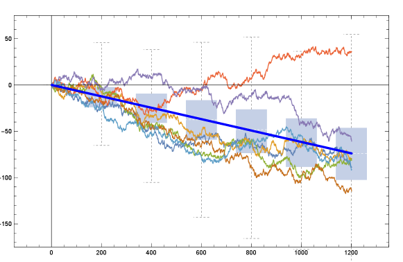
5 Opportunities and perils of random stepsizes
Here we investigate the implications of the variability arising from random stepsizes, see Figure 3. In §5.1, we show that trajectories can diverge but only with exponentially low probability. In §5.2, we investigate typical trajectories, showing that with overwhelming probability, their rate converges to the accelerated rate. In §5.3, we discuss running multiple trajectories in parallel and selecting the best.
5.1 Divergent runs and notion of convergence
When considering randomized optimization algorithms, there are several notions for measuring the convergence rate. Two natural ones are:
| (5.1) |
These are different. Indeed, our main result shows that by running GD with random stepsizes, the former quantity is asymptotically equal to the accelerated rate . Whereas the latter quantity can be larger than (details in Appendix B.3). Why the discrepancy between these two notions of convergence rate? Which is relevant for optimization?
The discrepancy arises because the error is exponentially small with overwhelming probability (leading to our convergence result for the first notion), but can be exponentially large with exponentially small probability (leading to the instability for the second notion). The key point is that for optimization algorithms, it is very desirable to succeed with overwhelming probability, even if performance is poor in the unlikely complement event. Simply re-run the algorithm if that happens. This why we study the quantity on the left hand side of (5.1). For intuition, we conclude this section with an illustrative toy example that explains this discrepancy in its simplest form.
Example 5.1 (Measuring convergence when exponentially rare trajectories can be exponentially large).
Consider i.i.d. random variables which are each equally likely to be or . Then by the Law of Large Numbers, hence
| (5.2) |
Whereas
| (5.3) |
In words, this discrepancy arises because can be exponentially large in , but the probability of this is exponentially small. For example, occurs with probability and thus by itself, this event contributes to the expectation in (5.3). Whereas the normalization inside the expectation in (5.2) dampens the effect of exponentially rare blow-ups, and thus agrees with the exponentially fast convergence that occurs with overwhelming probability.
5.2 Typical runs and high probability bounds
Theorem 1.2 establishes that random stepsizes lead to an accelerated rate in the limit as the number of iterations . The same analysis arguments can also establish non-asymptotic convergence rates that apply for any finite and hold with high probability. Indeed, recall from (3.2) that our argument in §3 relates the convergence rate (for any finite ) to an empirical sum, namely
| (5.4) |
Now, instead of using the Law of Large Numbers to argue that this empirical sum converges to its expectation (giving the accelerated rate), one can use concentration-of-measure to argue about the deviations from its expectation.
Below we state such a result. This is established by bounding the variance of the aforementioned empirical sum via a martingale-type argument and applying Chebyshev’s inequality; and then extending this convergence rate to general multivariate objectives by a union bound. Full proof details are deferred to Appendix B.4. We note that one can show more refined bounds by bounding higher-order moments or the moment generating function (see, e.g., the textbooks [55, 57, 17]), but that requires computing involved logarithmic integrals and thus for simplicity of exposition, here we state only this simple illustrative result.
Theorem 5.2 (Non-asymptotic version of Theorem 1.2).
This implies that for a typical run, the convergence rate is close to the accelerated rate; see Figure 3 for an illustration.
5.3 Best runs and parallelization
The randomness in the Arcsine Stepsize Schedule leads to a spread of convergence rates. Often the best run is substantially better than the median, which in turn is substantially better than the worst run; see Figure 3. This suggests a natural approach for parallelized optimization: run this randomized algorithm on different processors with i.i.d. stepsizes, and take the best final iterate. One can also perform a more refined parallelized scheme: synchronize every iterations by restarting all processors from the best current iterate.
How much of a speedup does this parallelization give? There are two sources of tension. First, the convergence rate achieved by Theorem 1.2 for processor is already minimax-optimal, but parallelization helps with instance-optimality which is important in practical settings, i.e., beyond worst-case settings. The second source of tension is that the results in §5.2 show that each of the i.i.d. runs has convergence rate concentrating around for large, which means that will be asymptotically unaffected by parallelization in the regime of fixed and . However, for regimes where and scale together, there are deviations from this concentration, and the maximal such deviation in the runs is precisely the speedup of this parallelization. See below for a calculation that illustrates this tension in a simple setting. Characterizing the tradeoff between the number of processors , the synchronization rate , the number of iterations , the condition number , and the precision is an interesting direction for future work but a full understanding is out of the scope of this paper.333Interesting phenomena arise when jointly optimizing and . For example, if , then moderate parallelism () improves the rate in both practice (see Figure 3) and theory (see below), but recovers exact line search which provably does not accelerate, see e.g., [9, §9.3]. This tradeoff warns of a potential drawback of over-parallelizing. On the other hand, when , the parallelization is a familiarly good algorithm: it produces the optimal point in the -dimensional Krylov subspace, which yields minimax-optimal worst-case convergence rates and is also instance-adaptive; in fact it is equivalent to Conjugate Gradients in exact arithmetic for quadratics.
Simple illustrative calculation.
Here, we provide a short back-of-the-envelope calculation in order to demonstrate these tensions and the benefit of parallelization in the simple setting of univariate quadratic functions. For simplicity consider a single synchronization (i.e., ); the general case of multiple synchronizations () follows by replacing by in this calculation, and then repeating this convergence rate times. For shorthand, let denote the -th iterate on the -th machine, let denote the corresponding stepsize, and let for (all univariate -conditioned quadratics are of this form).
Step 1: single machine. By the same analysis as in our main results (see §2.1 or §3.1) and then a Central Limit Theorem approximation, the convergence rate on the -th machine is
where and . Note that the error of this approximation can be tightly controlled using standard techniques such as the Berry-Esseen CLT [57, Theorem 2.1.13].
Step 2: best machine. Taking the minimum over all processors gives the convergence rate of the parallelized scheme which takes the best final iterate:
Above, the final step is due to the well-known fact that the minimum of i.i.d. standard Gaussians concentrates tightly around , see, e.g., [57, Chapter 2.5]. This factor quantifies the speedup of parallelization since it is the size of the variation in Figure 3. By a Taylor approximation of , this parallelization provides asymptotic speedups when , or equivalently when the number of processors .
6 Discussion and related results
6.1 Stability
Throughout, we have assumed for simplicity that all calculations are performed with exact gradients and in exact arithmetic. It is of practical importance to understand how inexactness affects convergence, and there is a long line of work on such questions for first-order algorithms, see, e.g., [16, 46, 18, 14, 51, 36, 1] and the references within. There are many models of inexact computation. Here, as an illustrative example, we study one common model: the multiplicative error model for gradients [16, 46]. Specifically, suppose that all calculations are still performed in exact arithmetic, but GD performs updates using an estimate of the true gradient , where
| (6.1) |
Theorem 6.1 (Inexact-gradient version of Theorem 1.2).
Consider the setup of Theorem 1.2. Suppose that GD updates in each iteration using rather than , i.e.,
| (6.2) |
where are inexact gradients satisfying the multiplicative-error assumption (6.1). Then the convergence rate of GD with i.i.d. Arcsine stepsizes is almost surely bounded by
| (6.3) |
Moreover this bound is tight, in that it holds with equality for some choice of and inexact gradients.
The proof is deferred to Appendix B.5, since it is similar to that of Theorem 1.2. Conceptually, the only difference is that the average Hessians are now perturbed, and thus the convergence rate is governed by where can now be slightly outside the interval .
We remark that for small error , the slowdown factor in Theorem 6.1 is of the order
In other words, for large condition number , the number of iterations required by GD increases by a multiplicative factor of roughly when using inexact gradients. Note that this slowdown is more than the slowdown for constant-stepsize schedules [16, Theorem 5.3]. This is a manifestation of the general phenomenon that accelerated algorithms are often less stable to model mis-specification, see e.g., [18].
We also remark that by a nearly identical argument, Theorem 6.1 can be extended to a stochastic error models, i.e., where are random. The slowdown factor then becomes an averaged version of the quantity in Theorem 6.1. However, this is more complicated to state, hence for simplicity the above discussion focuses just on the deterministic error model.
6.2 Game-theoretic connections and lower bounds
This paper considers random stepsizes for the algorithmic purpose of accelerating GD. It turns out that this randomized perspective is also helpful for the dual problem of constructing algorithmic lower bounds. We describe this duality here.
Recall from §2 that the optimal distribution over i.i.d. inverse stepsizes has the following extremal characterization:
| (6.4) |
Above, is constrained to without loss of generality (since this holds at optimality), should be interpreted as the curvature of a “worst-case” univariate quadratic function , and is the logarithm of the asymptotic convergence rate.
To bridge this problem of accelerating GD with the problem of constructing lower bounds, we consider a standard two-player zero-sum game where players choose their actions simultaneously and independently. In our case, one player chooses inverse stepsizes and the other player chooses a quadratic function (parameterized by its curvature . By lifting to mixed (i.e., randomized) strategies, one player chooses a distribution over stepsizes, the other chooses a distribution over quadratic functions, with payoff given by .
The key observation is that due to the specific payoff function, the game is essentially symmetric between the two players (modulo inversion), and as a consequence, so are the optimal mixed strategies for both players. Below, let denote the law of when .
Lemma 6.2 (Optimal distribution for worst-case functions).
The (minimax) value of this game is , i.e., we have the saddle point condition
with
and the unique optimal mixed strategies are and .
Remark 6.3 (Game-theoretic interpretation of equalization).
Notice that both optimal distributions have full support. As a consequence, at equilibrium a player is indifferent among all of their pure actions, i.e., the equalization property (Lemma 2.2) must hold.
Proof sketch for Lemma 6.2.
Lemma 2.1 implies that is the unique optimal solution for the stepsize player, and that the value of the game is . See [2, Chapter 3.3.3] for a rigorous proof that the unique optimal solution for the other player is ; here we just provide intuition in terms of symmetry of the game. The underlying idea is to consider a “flipped game” in which strategies correspond to the inverses of strategies in the original game, i.e., one player chooses stepsizes , and the other player chooses a quadratic function parameterized by its inverse curvature . Here where and . By lifting to mixed strategies, one player chooses a distribution over stepsizes , and the other player chooses a distribution over quadratic functions , with payoff given by
This flipped game is equivalent to the original game due the invariance of both the payoff function and the condition number with respect to this inversion of the strategies. Because is the unique optimal solution in the original game, is the unique optimal solution in the flipped game; in order to show that is the unique optimal solution in the original game, it suffices to show that is the unique optimal solution in the flipped game. To this end, it suffices to show that an optimal solution must satisfy the equalization property in the flipped game, i.e.,
is independent of . This suffices since the equalization property uniquely defines the Arcsine distribution by classical results from logarithmic potential theory, see Appendix A.
Why must an optimal solution for the flipped game satisfy this equalization property? An informal argument is as follows. By definition of , the symmetry between and , and then the equalization property of the Arcsine distribution (Lemma 2.2) applied to ,
Thus, forgoing measure-theoretic technicalities, if did not satisfy the equalization property, then by the probabilistic method, there would exist some for which is strictly less than its average . But this means that the value of the flipped game is less than , hence also for the original game (since their values are identical), contradiction. ∎
As a corollary, Lemma 6.2 gives a new proof that is the fastest possible convergence rate for GD. This result is classically due to [39], who proved this by constructing a single, infinite-dimensional “worst-case function” for which any Krylov-subspace algorithm converges slowly. Here we construct a “worst-case distribution” over univariate functions for which any GD stepsize schedule converges slowly in expectation. By the probabilistic method, for any specific GD stepsize schedule, we can then conclude the existence of a single univariate function for which convergence is slow. For simplicity, we state this lower bound here for i.i.d. stepsizes; this can be extended to arbitrary GD stepsize schedules and also to non-asymptotic lower bounds, see [2, Chapter 5].
Corollary 6.4.
For any distribution of i.i.d. GD stepsizes, there exists a univariate quadratic function that is -strongly convex and -smooth such that the asymptotic convergence rate
Proof.
Lemma 6.2 shows that in expectation over , the asymptotic convergence rate is when run on the quadratic function from initialization . By the probabilistic method, there exists a for which the asymptotic convergence rate on is at least this average value . ∎
Remark 6.5.
The lower bounds in this section can be interpreted as an instantiation of Yao’s minimax principle [60]: in order to lower bound the performance of a randomized algorithm (e.g., GD with the Arcsine Stepsize Schedule), we exhibit a distribution over difficult inputs (namely quadratics with curvature according to the FlippedArcsine distribution) for which any deterministic algorithm cannot perform well. This is implicit along the way in this section’s development.
7 Conclusion and future work
This paper shows that randomizing stepsizes provides an alternative mechanism for accelerated convex optimization beyond the special case of quadratics. This raises several natural questions about the possible benefit of randomness for GD—or said equivalently, whether the Arcsine Stepsize Schedule can be derandomized. The current results differ on two fronts: Theorem 1.2 shows that random stepsizes achieve the fully accelerated rate on separable functions, whereas [3] shows that deterministic stepsize achieves the partially accelerated “Silver” rate on general convex functions. These two sources of differences motivate the questions:
-
•
Is it possible to de-randomize Theorem 1.2, i.e., construct a deterministic stepsize schedule which achieves the fully accelerated rate for separable functions? If so, a natural conjecture would be some ordering of the Chebyshev stepsize schedule.
-
•
Does the Arcsine Stepsize Schedule fully accelerate on general (non-separable) convex functions? If not, can any randomized stepsize schedule improve over the Silver Convergence Rate for general convex functions?
There are also many questions about extensions to other optimization settings of interest. For other settings, what is the optimal stepsize distribution if not Arcsine? In any setting, is there a provable benefit of using non-i.i.d. stepsizes? Can random stepsizes be alternatively understood through discretization analyses of continuous-time gradient flows? While other mechanisms for acceleration (e.g., momentum) are now well understood [22], little is known about acceleration via randomness.
Appendix A Connections to logarithmic potential theory
Recall from the overview section §2 that the optimal distribution for inverse stepsizes is given by the extremal problem
| (A.1) |
where and denotes the probability distributions supported on .444Although the stepsize problem was not originally written with this constraint in §2, it is easily seen that this constraint is satisfied at optimality and therefore does not change the extremal problem. See Observation A.4. Indeed, for quadratic optimization, this extremal problem exactly characterizes the asymptotic convergence rate (see §2.1); and for the more general setting of separable convex optimization, even though the relevant extremal problem is somewhat different, the solution is identical (see §2.2).
In this appendix section, we connect this extremal problem over stepsize distributions with the extremal problem for electrostatic capacitors that is classically studied in potential theory. As we explain below, although these two problems seek probability distributions minimizing different objectives, the two problems are intimately linked because they have the same optimality condition: the optimal distribution must satisfy the equalization property from Lemma 2.2 (i.e., the objective has equal value for all ). Because this equalization property uniquely characterizes the distribution (a classical fact from potential theory, see Lemma A.9), this means that the two problems have the same unique optimal solution. In this way, the equalization property plays the central role connecting these two problems.
This appendix section is organized as follows. In §A.1 we recall the electrostatics problem and highlight the syntactic similarities and differences to the stepsize problem. In §A.2 we explain the equalization property in the context of both problems and how it arises as the optimality condition. This is the key link between the two problems. In §A.3 we exploit this connection concretely by using the machinery of potential theory to solve the stepsize problem. This provides alternative proofs of Lemmas 2.1 and 2.2 that are significantly shorter than the integral calculations of [32, 47].
A.1 Extremal problem for electrostatic capacitors
The extremal problem central to logarithmic potential theory is
| (A.2) |
given a set . This problem is sometimes called the electrostatics problem for a capacitor due to its physical interpretation: how should you place a distribution of repelling particles on so as to minimize the total repulsive energy? Here the repulsive energy is measured via
which is the -average of the logarithmic potential energy at , denoted
Standard arguments based on lower semi-continuity and strict convexity of the objective ensure that an optimal distribution exists and is unique. For certain sets , this optimal distribution can be computed in closed form. For example it is well-known that for the interval , the unique optimal distribution is the distribution, see e.g., [49, Example 1.11].
Syntactic similarities and differences.
Let . Then the stepsize extremal problem (A.1) clearly bears similarities to the electrostatics extremal problem (A.2), namely
| (A.3) |
Yet there are two differences. First, the stepsize problem evaluates the logarithmic potential at a specific point , whereas the electrostatics problem averages this potential over . Second, the stepsize problem has an additional term of .
In general, changing the objective or constraints in an extremal problem can significantly alter the optimal solution. Yet, remarkably, the optimal solution is identical for both problems. This is because both problems have the same optimality condition, described next.
A.2 Equalization property
Here we describe how the equalization property arises as the optimality condition in both problems.
A.2.1 Equalized potential for the electrostatics problem
A celebrated fact—sometimes called the Fundamental Theorem of Potential Theory [48, Chapter 3.3]—is that the optimal distribution to the electrostatics problem (A.2) satisfies an equalization property: the potential is constant on . (Note that this is equivalent to the constancy on of the objective for the stepsize problem, namely .)
This equalization property has an intuitive physical interpretation: if the potential is not constant on , then particles will flow to points of with lower potential, so the current state is not at equilibrium and therefore cannot be optimal. This is why the optimal solution is often called the equilibrium distribution. This result is attributed to Frostman; here we state a simple version of it that suffices for our setting (namely a compact interval ).
Theorem A.1 (Frostman’s Theorem).
A proof can be found in any textbook on logarithmic potential theory, e.g., [54, 48, 50]. Below we use calculus of variations to give an informal back-of-the-envelope calculation that provides intuition for how this equalization property arises as the optimality condition. Let
denote the original objective plus a Lagrangian term for the normalization constraint on . Then a quick calculation shows that the first variation is
In order for this first variation to vanish along any direction , it must hold that
This is the equalization property.
A.2.2 Equalized convergence rate for the stepsize problem
As discussed in §2.1 and formally stated in Lemma 2.1, the stepsize problem has the same equalization property at optimality. This is rigorously proven in §A.3.2 using the machinery of potential theory; to provide intuition for how this arises as the optimality condition, here we give an informal back-of-the-envelope argument based on the game-theoretic perspective developed in §6.2.
Suppose that is an solution to the stepsize problem (A.1). By the calculation in §6.2, there is a distribution (the Flipped Arcsine distribution) for which
| (A.4) |
Observe that this is the -average of . Thus, if does not equalize, then (forgoing measure-theoretic technicalities) there exists for which is strictly larger than the -average. That is, . But this contradicts the optimality of since the value of the stepsize problem (A.1) is . Therefore the equalization property must be satisfied by the optimal distribution .
A.3 Solution to the extremal problem over stepsizes
So far we have focused on developing conceptual connections between the stepsize problem and electrostatistics problem. We now exploit these connections concretely by using the machinery of potential theory to solve the stepsize problem. This provides short proofs of Lemmas 2.1 and 2.2.
A.3.1 Proof of Lemma 2.2
Here we prove the equalization property. In the optimization literature, this was proven by computing the integral directly using trigonometric identities [47], or by decomposing the logarithmic integrand into the Chebyshev polynomial basis [32]. Here we mention an alternative approach by appealing to the following well-known identity from potential theory, which gives the potential for the equilibrium distribution on at any point ; see e.g., [50, Example 1.11].
Fact A.2.
Let denote the Arcsine distribution on . Then for any ,
Proof of Lemma 2.2.
Let denote the Arcsine distribution on . Note that is the push-forward of under the linear map that sends to . Thus by a change-of-measure, the -potential at any is
where . This gives the desired identity:
Above the first step is by expanding the logarithm, the second step is by definition of the logarithmic potential , the third step is by Fact A.2 and the above formula for in terms of , and the last step is by plugging in the value of and simplifying. ∎
Remark A.3 (Connection to Green’s function).
This expression is the evaluation at of Green’s function for the interval . This connection essentially arises because: 1) for quadratic optimization, polynomial approximation dictates the convergence rate of GD (see §2.1), and 2) the Bernstein-Walsh Theorem characterizes the optimal rate of convergence of polynomial approximations in terms of Green’s function (see e.g., [19, Theorem 1]).
A.3.2 Proof of Lemma 2.1
Here we prove that the Arcsine distribution is the unique optimal solution for the stepsize problem (A.1) by mirroring the standard argument from potential theory that the Arcsine distribution is the unique optimal solution to the electrostatic problem (A.2), see e.g., [49, Example 2.9]. Specifically, our approach is to show that any optimal distribution satisfies the equalization property (see §A.2.2 for a heuristic argument of this). Indeed, it then follows that the optimal distribution is unique and is the Arcsine distribution by the converse of Frostman’s Theorem (stated below), which ensures that the Arcsine distribution is the unique distribution satisfying equalization.
We begin with a simple observation.
Observation A.4 (Support of the optimal stepsize distribution).
The constraint does not change the value of the stepsize problem (A.1).
Proof.
It suffices to argue that for any distribution (with arbitrary support), there exists some distribution whose objective value is at least as good, i.e., . To this end, it suffices to observe the elementary inequality
where is arbitrary and is the projection of onto the interval . Indeed, this pointwise inequality implies that we can project onto in this way without worsening the objective value of . ∎
We now show that any optimal distribution, constrained to this interval, must satisfy the equalization property. For this it is helpful to recall several classical facts from potential theory. These can be found, e.g., in page 171 and Theorems 3.2, 2.8, 2.2, and 3.1, respectively, of [49].
Lemma A.5 (Basic properties of logarithmic potentials).
If , then is lower semicontinuous on and harmonic outside the support of .
Lemma A.6 (Continuity of the equilibrium potential).
Consider the setting of Theorem A.1. Then the potential is continuous on .
Lemma A.7 (Principle of domination).
Suppose are compactly supported and that . If for some constant , holds -a.e., then it holds for all .
Lemma A.8 (Maximum principle).
Suppose is a harmonic function on a domain . If attains a local maximum in , then is constant on .
Lemma A.9 (Converse to Frostman’s Theorem).
Suppose satisfies . If on for some constant , then is the equilibrium distribution for .
Proof of Lemma 2.1.
For shorthand, let denote the distribution and note that by Lemma 2.2. Suppose has objective value for the stepsize problem (2.9) that is at least as good as . Then by the equalization property for (Lemma 2.2),
Re-arranging gives
| (A.5) |
where and . By the principle of domination (Lemma A.7), this inequality (A.5) holds for all . Since , we conclude that achieves its maximum on at . But because is harmonic on (Lemma A.5), the Maximum Principle (Lemma A.8) implies that is constant on , i.e.,
| (A.6) |
Fix any and let be any sequence in converging to . Note that by lower semicontinuity (Lemma A.5), and by continuity of the equilibrium potential (Lemma A.6). Thus by (A.6),
Combining this with (A.5) shows that
Thus has constant logarithmic potential on , and therefore by the converse to Frostman’s Theorem (Lemma A.9), it must be the equilibrium distribution, a.k.a., . We conclude that the Arcsine distribution is the unique optimal solution for the stepsize problem (A.1). The optimal value then follows from Lemma 2.1. ∎
Appendix B Deferred proofs
B.1 Equivalence of separability and commutative Hessians
Here we prove an alternative characterization of separability. We remark that this provides a simple way to certify that a function is not separable: it suffices to exhibit points and for which the Hessians and do not commute.
Lemma B.1 (Equivalence of separability and commutative Hessians).
Let . Then the following are equivalent:
-
(i)
where for some orthogonal and functions .
-
(ii)
commute.
Proof of (i) (ii). The function is separable, hence its Hessian is diagonal. The chain rule implies , thus the Hessians of are simultaneously diagonalizable in the basis , hence they commute.
Proof of (ii) (i). Since the Hessians commute, they are simultaneously diagonalizable, i.e., there exists an orthogonal matrix such that for all , where is diagonal. Defining , it follows by the chain rule that is diagonal. Thus all mixed partial derivatives vanish, hence is a function only of .
Integrating implies for some functions . Thus as desired.
B.2 Proof of Lemma 3.2
We first isolate a useful identity: the random variables defined in §3.1 are uncorrelated—despite not being independent. Intuitively, this is due to the equalization property of the Arcsine distribution (from which are independently drawn) since it ensures that each has the same (conditional) expectation regardless of the dependencies injected through the non-stationary process .
Lemma B.2.
for all .
Proof.
Proof of Lemma 3.2.
First we check that is indeed a martingale:
The final step uses , which follows by an identical argument as in (3.3) above.
Next, we show is -bounded. By the Cauchy-Schwarz inequality,
Thus it suffices to show that is uniformly bounded away from . To this end, since for any by Lemma B.2, it follows that
where is a uniform upper bound on the variance of . Note that because the logarithmic potential is an integrable singularity (see also Appendix 5 of [32] for quantitative bounds on ). Thus has finite variance, as desired. ∎
B.3 Details for §5.1
Here we observe that random stepsizes can make GD unstable in alternative notions of convergence. Instability in the following lemma occurs for since then . See §5.1 for a discussion of this phenomena and why the notion of convergence studied in the rest of this paper is more relevant to optimization practice.
Lemma B.3 (Instability in alternative notions of convergence).
Consider GD with i.i.d. inverse stepsizes from . There is an -strongly convex, -smooth, quadratic function such that for any initialization and any number of iterations ,
| (B.1) |
To prove this, we make use of the following integral representation of the geometric mean of two positive scalars in terms of the weighted harmonic mean . This identity is well-known (e.g., it follows from [7, Exercise V.4.20], or directly from [25, §3.121-2] by taking and ).
Lemma B.4 (Arcsine integral representation of the geometric mean).
For any ,
This lets us compute the expectation of the proposed random stepsizes.
Lemma B.5 (Expectation of proposed random stepsizes).
For any ,
Proof.
We are now ready to prove Lemma B.3.
Proof of Lemma B.3.
Let denote the inverse stepsizes; recall that these are i.i.d. . By expanding the definition of GD for the function ,
By taking expectations, using independence of the stepsizes, and applying Lemma B.5,
Thus by Jensen’s inequality and then the fact that , we conclude the desired inequality
∎
B.4 Proof of Theorem 5.2
For shorthand, let denote a uniform upper bound on the variance of any . By the integral calculations in [32, Appendix 5],
Thus because for by Lemma B.2,
Thus by Chebyshev’s inequality and the equalization property of the Arcsine distribution (Lemma 2.2),
| (B.2) |
where are i.i.d. and is any process adapted to the filtration . Thus by (3.2), the average convergence rate for the function satisfies
| (B.3) |
for any coordinate , i.e., for any for which the initialization is not already optimal. Thus the overall convergence rate for satisfies
| (B.4) |
Above the first step is because (since ). The second step is by a union bound and the previous display. The proof is then complete by setting equal to the right hand side of the above display.
B.5 Details for §6.1
Proof of Theorem 6.1.
The proof is similar to that of Theorem 1.2, so we just highlight the differences. By the same argument as in §3.2, it suffices to show the result for univariate objectives , so we henceforth restrict to this case. For shorthand, denote and note that the multiplicative error assumption (6.1) implies by smoothness. By an identical calculation as in §3.1,
and thus
and so in particular
By a similar martingale-based Law of Large Numbers argument as in §3.1, it suffices to compute
| (B.5) |
and in particular to show that this equal to the logarithm of the upper bound in (6.3). Above, plays the role of where and . By the same calculation as in Appendix A.3.1, this expectation simplifies to
| (B.6) |
where . This quantity is increasing in , thus (B.5) is maximized at both extremes which lead to the same maximal value of . Plugging this into (B.5) yields the desired bound.
Finally, for tightness, note that the analysis is tight at the aforementioned extremes and . These two extremes respectively correspond to functions and , with estimates that maximally underestimate or overestimate the true gradient. ∎
References
- Agarwal et al. [2021] Naman Agarwal, Surbhi Goel, and Cyril Zhang. Acceleration via fractal learning rate schedules. In International Conference on Machine Learning, pages 87–99. PMLR, 2021.
- Altschuler [2018] Jason M. Altschuler. Greed, hedging, and acceleration in convex optimization. Master’s thesis, Massachusetts Institute of Technology, 2018.
- Altschuler and Parrilo [2023] Jason M Altschuler and Pablo A Parrilo. Acceleration by Stepsize Hedging I: Multi-Step Descent and the Silver Stepsize Schedule. arXiv preprint arXiv:2309.07879, 2023.
- Altschuler and Parrilo [2024] Jason M Altschuler and Pablo A Parrilo. Acceleration by Stepsize Hedging: Silver Stepsize Schedule for Smooth Convex Optimization. Mathematical Programming, pages 1–14, 2024.
- Barzilai and Borwein [1988] Jonathan Barzilai and Jonathan M Borwein. Two-point step size gradient methods. IMA Journal of Numerical Analysis, 8(1):141–148, 1988.
- Bertsekas [1999] Dimitri P. Bertsekas. Nonlinear programming. Athena Scientific, 1999.
- Bhatia [2013] Rajendra Bhatia. Matrix analysis, volume 169. Springer Science & Business Media, 2013.
- Bok and Altschuler [2024] Jinho Bok and Jason M. Altschuler. Accelerating proximal gradient descent via silver stepsizes. arXiv preprint, 2024.
- Boyd and Vandenberghe [2004] Stephen Boyd and Lieven Vandenberghe. Convex optimization. Cambridge University Press, 2004.
- Bubeck [2015] Sébastien Bubeck. Convex optimization: Algorithms and complexity. Foundations and Trends in Machine Learning, 8(3-4):231–357, 2015.
- Bubeck et al. [2015] Sébastien Bubeck, Yin Tat Lee, and Mohit Singh. A geometric alternative to Nesterov’s accelerated gradient descent. arXiv preprint arXiv:1506.08187, 2015.
- Daccache [2019] Antoine Daccache. Performance estimation of the gradient method with fixed arbitrary step sizes. PhD thesis, Master’s thesis, Université Catholique de Louvain, 2019.
- Das Gupta et al. [2023] Shuvomoy Das Gupta, Bart PG Van Parys, and Ernest K Ryu. Branch-and-bound performance estimation programming: a unified methodology for constructing optimal optimization methods. Mathematical Programming, pages 1–73, 2023.
- d’Aspremont [2008] Alexandre d’Aspremont. Smooth optimization with approximate gradient. SIAM Journal on Optimization, 19(3):1171–1183, 2008.
- De Klerk et al. [2017] Etienne De Klerk, François Glineur, and Adrien B Taylor. On the worst-case complexity of the gradient method with exact line search for smooth strongly convex functions. Optimization Letters, 11:1185–1199, 2017.
- De Klerk et al. [2020] Etienne De Klerk, Francois Glineur, and Adrien B Taylor. Worst-case convergence analysis of inexact gradient and Newton methods through semidefinite programming performance estimation. SIAM Journal on Optimization, 30(3):2053–2082, 2020.
- Dembo [2009] Amir Dembo. Large deviations techniques and applications. Springer, 2009.
- Devolder et al. [2014] Olivier Devolder, François Glineur, and Yurii Nesterov. First-order methods of smooth convex optimization with inexact oracle. Mathematical Programming, 146:37–75, 2014.
- Driscoll et al. [1998] Tobin A Driscoll, Kim-Chuan Toh, and Lloyd N Trefethen. From potential theory to matrix iterations in six steps. SIAM Review, 40(3):547–578, 1998.
- Drori and Teboulle [2014] Yoel Drori and Marc Teboulle. Performance of first-order methods for smooth convex minimization: a novel approach. Mathematical Programming, 145(1-2):451–482, 2014.
- Drusvyatskiy et al. [2018] Dmitriy Drusvyatskiy, Maryam Fazel, and Scott Roy. An optimal first order method based on optimal quadratic averaging. SIAM Journal on Optimization, 28(1):251–271, 2018.
- d’Aspremont et al. [2021] Alexandre d’Aspremont, Damien Scieur, and Adrien Taylor. Acceleration methods. Foundations and Trends® in Optimization, 5(1-2):1–245, 2021.
- Eloi [2022] Diego Eloi. Worst-case functions for the gradient method with fixed variable step sizes. PhD thesis, Master’s thesis, Université Catholique de Louvain, 2022.
- Goujaud et al. [2022] Baptiste Goujaud, Damien Scieur, Aymeric Dieuleveut, Adrien B Taylor, and Fabian Pedregosa. Super-acceleration with cyclical step-sizes. In International Conference on Artificial Intelligence and Statistics, pages 3028–3065. PMLR, 2022.
- Gradshteyn and Ryzhik [2014] Izrail Solomonovich Gradshteyn and Iosif Moiseevich Ryzhik. Table of integrals, series, and products. Academic Press, 2014.
- Grimmer [2024] Benjamin Grimmer. Provably faster gradient descent via long steps. SIAM Journal on Optimization, 34(3):2588–2608, 2024.
- Grimmer et al. [2023] Benjamin Grimmer, Kevin Shu, and Alex L. Wang. Accelerated gradient descent via long steps. arXiv preprint arXiv:2309.09961, 2023.
- Grimmer et al. [2024a] Benjamin Grimmer, Kevin Shu, and Alex Wang. Accelerated objective gap and gradient norm convergence for gradient descent via long steps. arXiv preprint arXiv:2403.14045, 2024a.
- Grimmer et al. [2024b] Benjamin Grimmer, Kevin Shu, and Alex L Wang. Composing optimized stepsize schedules for gradient descent. arXiv preprint arXiv:2410.16249, 2024b.
- Hazan [2016] Elad Hazan. Introduction to online convex optimization. Foundations and Trends in Optimization, 2(3-4):157–325, 2016.
- Hestenes et al. [1952] Magnus R Hestenes, Eduard Stiefel, et al. Methods of conjugate gradients for solving linear systems. Journal of Research of the National Bureau of Standards, 49(6):409–436, 1952.
- Kalousek [2017] Zdeněk Kalousek. Steepest descent method with random step lengths. Foundations of Computational Mathematics, 17(2):359–422, 2017.
- Kelley [1999] Carl T Kelley. Iterative methods for optimization. SIAM, 1999.
- Kelner et al. [2022] Jonathan Kelner, Annie Marsden, Vatsal Sharan, Aaron Sidford, Gregory Valiant, and Honglin Yuan. Big-step-little-step: Efficient gradient methods for objectives with multiple scales. In Conference on Learning Theory, pages 2431–2540. PMLR, 2022.
- Lan [2020] Guanghui Lan. First-order and stochastic optimization methods for machine learning, volume 1. Springer, 2020.
- Lebedev and Finogenov [1971] VI Lebedev and SA Finogenov. Ordering of the iterative parameters in the cyclical Chebyshev iterative method. USSR Computational Mathematics and Mathematical Physics, 11(2):155–170, 1971.
- Lessard et al. [2016] Laurent Lessard, Benjamin Recht, and Andrew Packard. Analysis and design of optimization algorithms via integral quadratic constraints. SIAM Journal on Optimization, 26(1):57–95, 2016.
- Luenberger and Ye [1984] David G Luenberger and Yinyu Ye. Linear and nonlinear programming, volume 2. Springer, 1984.
- Nemirovskii and Yudin [1983] Arkadii Nemirovskii and David Borisovich Yudin. Problem complexity and method efficiency in optimization. Wiley, 1983.
- Nesterov [1998] Yurii Nesterov. Introductory lectures on convex optimization: A basic course, volume 87. Springer Science & Business Media, 1998.
- Nesterov [1983] Yurii E. Nesterov. A method of solving a convex programming problem with convergence rate . Soviet Math. Dokl., 27(2):372–376, 1983.
- Nocedal and Wright [1999] J. Nocedal and S. J. Wright. Numerical Optimization. Springer, 1999.
- Oymak [2021] Samet Oymak. Provable super-convergence with a large cyclical learning rate. IEEE Signal Processing Letters, 28:1645–1649, 2021.
- Polyak [1964] Boris T Polyak. Some methods of speeding up the convergence of iteration methods. USSR Computational Mathematics and Mathematical Physics, 4(5):1–17, 1964.
- Polyak [1987] Boris T. Polyak. Introduction to optimization. Optimization Software, Inc., 1987.
- Polyak [1971] Boris Teodorovich Polyak. Convergence of methods of feasible directions in extremal problems. USSR Computational Mathematics and Mathematical Physics, 11(4):53–70, 1971.
- Pronzato and Zhigljavsky [2011] Luc Pronzato and Anatoly Zhigljavsky. Gradient algorithms for quadratic optimization with fast convergence rates. Computational Optimization and Applications, 50(3):597–617, 2011.
- Ransford [1995] Thomas Ransford. Potential theory in the complex plane, volume 28. Cambridge University Press, 1995.
- Saff [2010] Edward B Saff. Logarithmic potential theory with applications to approximation theory. Surveys in Approximation Theory, 5:165–200, 2010.
- Saff and Totik [2013] Edward B Saff and Vilmos Totik. Logarithmic potentials with external fields, volume 316. Springer Science & Business Media, 2013.
- Schmidt et al. [2011] Mark Schmidt, Nicolas Roux, and Francis Bach. Convergence rates of inexact proximal-gradient methods for convex optimization. Advances in neural information processing systems, 24, 2011.
- Taylor and Drori [2023] Adrien Taylor and Yoel Drori. An optimal gradient method for smooth strongly convex minimization. Mathematical Programming, 199(1-2):557–594, 2023.
- Taylor et al. [2017] Adrien B Taylor, Julien M Hendrickx, and François Glineur. Smooth strongly convex interpolation and exact worst-case performance of first-order methods. Mathematical Programming, 161(1-2):307–345, 2017.
- Tsuji [1959] Masatsugu Tsuji. Potential theory in modern function theory. Maruzen, 1959.
- Van Handel [2014] Ramon Van Handel. Probability in high dimension. Lecture Notes (Princeton University), 2(3):2–3, 2014.
- Van Scoy et al. [2018] Bryan Van Scoy, Randy A Freeman, and Kevin M Lynch. The fastest known globally convergent first-order method for minimizing strongly convex functions. IEEE Control Systems Letters, 2(1):49–54, 2018.
- Vershynin [2018] Roman Vershynin. High-dimensional probability: An introduction with applications in data science, volume 47. Cambridge University Press, 2018.
- Wang et al. [2024] Bofan Wang, Shiqian Ma, Junfeng Yang, and Danqing Zhou. Relaxed proximal point algorithm: Tight complexity bounds and acceleration without momentum. arXiv preprint arXiv:2410.08890, 2024.
- Williams [1991] David Williams. Probability with martingales. Cambridge University Press, 1991.
- Yao [1977] Andrew Chi-Chin Yao. Probabilistic computations: Toward a unified measure of complexity. In Symposium on Foundations of Computer Science (FOCS), pages 222–227. IEEE, 1977.
- Young [1953] David Young. On Richardson’s method for solving linear systems with positive definite matrices. Journal of Mathematics and Physics, 32(1-4):243–255, 1953.
- Zhang and Jiang [2024] Zehao Zhang and Rujun Jiang. Accelerated gradient descent by concatenation of stepsize schedules. arXiv preprint arXiv:2410.12395, 2024.
- Zhigljavsky et al. [2013] Anatoly Zhigljavsky, Luc Pronzato, and Elena Bukina. An asymptotically optimal gradient algorithm for quadratic optimization with low computational cost. Optimization Letters, 7(6):1047–1059, 2013.