Accounting for Cosmic Variance in Studies of Gravitationally-Lensed High-Redshift Galaxies in the Hubble Frontier Field Clusters

The remarkable capabilities of Wide Field Camera 3 (WFC3) on Hubble Space Telescope (HST) have transformed infrared extragalactic surveys of the distant universe. The Cosmic Assembly Near-infrared Deep Extragalactic Legacy Survey (CANDELS: Grogin et al., 2011; Koekemoer et al., 2011), the Cluster Lensing And Supernova survey with Hubble (CLASH: Postman et al., 2012), and the Ultra Deep Field surveys (UDF: Beckwith et al., 2006; Ellis et al., 2013; Koekemoer et al., 2013; Illingworth et al., 2013) have provided critical new information about the rest-frame ultraviolet properties of early galaxies, their redshift-dependent abundance, and the development of morphological structures over time (e.g., McLure et al., 2010; Oesch et al., 2010; Bouwens et al., 2011; Finkelstein et al., 2012; Schenker et al., 2013; McLure et al., 2013; Dunlop et al., 2013; Ono et al., 2013; Curtis-Lake et al., 2014).

The deepest HST observations to date in the UDF have reached multi-band sensitivities of $m_{\mathrm{AB}}\approx 29.5-30$ (e.g., Ellis et al., 2013) after a total exposure of hundreds of hours in a “blank” (i.e., devoid of strong lensing) field. To supplement the high-redshift galaxy populations discovered in the UDF and its parallel fields, the currently on-going Frontier Fields program (Program ID 13495; PI Lotz, Co-PI Mountain) utilizes carefully selected strong gravitational lens clusters to probe intrinsically fainter limits through high magnifications. With the ability to detect galaxies with intrinsic magnitudes as faint as $m_{\mathrm{AB}}\sim 32$, the Frontier Fields program has the potential to constrain the galaxy luminosity function faint-end slope at redshifts $z>6$ and probe the UV luminosity density out to $z\sim 12$. Such constraints can provide vital clues to the process of cosmic reionization (Robertson et al., 2010), as previous analyses have suggested that the ionizing photon budget at $z\sim 7$ is dominated by faint galaxies below the current UDF limits (e.g., Robertson et al., 2013). Indeed, the first Frontier Fields observations of the cluster Abell 2744 (A2744) have already been used to identify galaxy candidates in the reionization epoch (Atek et al., 2014a, b; Zheng et al., 2014; Zitrin et al., 2014; Ishigaki et al., 2014) and to constrain the luminosity density at redshift $z\sim 10$ (Oesch et al., 2014). These results complement discoveries of strongly-lensed high-redshift galaxies in the CLASH survey (Zheng et al., 2012; Coe et al., 2013; Bradley et al., 2014).

Utilizing lensed observations to infer constraints on the early galaxy populations requires careful considerations of the volumes probed and the associated uncertainties. This Letter presents the first estimates of the cosmic variance of high-redshift galaxy samples in the Frontier Fields (FF) survey. Using the publicly-available magnification maps for the first FF cluster, Abell 2744, we estimate the effective survey volume as a function of magnification and calculate the associated cosmic variance uncertainty. Since the magnification varies significantly across a given cluster lens, we use the connection between magnification, effective survey volume, and cosmic variance uncertainty to produce a “cosmic variance map”. Importantly, in regions of extreme magnification, where the gain of lensing is most valuable, the cosmic variance uncertainty is increased relative to that for comparable blank-field surveys. This uncertainty has important implications for the benefits of the FF program in its stated goals, as we attempt to quantify.

Throughout this Letter we adopt the flat $\Lambda$CDM cosmology ($\Omega_{m}=0.3$, $\Omega_{\Lambda}=0.7$, $h=0.7$) used to produce the Richard et al. (2014) lensing maps of A2744. We further adopt the normalization of the linear power spectrum $\sigma_{8}=0.829$, spectral index $n=0.96$, and baryon density $\Omega_{b}=0.0487$ measured by Planck Collaboration et al. (2013).

The cosmic variance (CV) uncertainty of an observed galaxy population reflects fluctuations in the matter density about the mean cosmic density, as sampled by the survey volume. In linear theory, the galaxy number density $n$ in a volume will differ from the mean number density $\bar{n}$ as $n=\bar{n}(1+b\delta)$, where $\delta$ is the matter overdensity in the survey volume, and $b$ is the clustering bias of the galaxy population.

The bias $b$ and survey volume probed will in general depend on the galaxy luminosity, which is important in the context of a strong lens survey where the effective volume varies strongly with intrinsic source flux. In an unlensed blank field, the sample covariance matrix $S_{ij}=\langle(n_{i}-\bar{n}_{i})(n_{j}-\bar{n}_{j})\rangle$ of the number of galaxies $n_{i}$ and $n_{j}$ in luminosity or magnitude bins $i$ and $j$ depends on the bias of the galaxy populations $b_{i}$ and $b_{j}$, and the average numbers of galaxies $\bar{n}_{i}$ and $\bar{n}_{j}$ expected in the survey (for details see, e.g., Robertson, 2010a, b).

The diagonal terms $S_{ii}$ of this matrix provide the cosmic variance $\sigma_{\mathrm{CV}}^{2}$ of the total galaxy number counts typically expressed as a fractional uncertainty

where $\langle\ldots\rangle_{i}$ denotes a suitable averaging of the luminosity-dependent bias of the observed sample, and results in the product of an average bias $\langle b\rangle$, the growth factor $D(z)$, and the rms matter density fluctuations $\sigma_{DM}$ in the survey volume at $z=0$ assuming the effective survey geometry is luminosity-independent (see Sections 2.3 and 2.4 of Robertson, 2010b). In the absence of direct clustering constraints, we estimate the bias $b$ by using abundance matching (Kravtsov et al., 2004; Conroy et al., 2006) to assign dark matter masses to galaxies based on the Tinker et al. (2008) halo mass function and then applying the bias model of Tinker et al. (2010).

To estimate the sample variance $S_{ii}$ of a galaxy population with a range of magnifications, some averaging is needed. For any intrinsic luminosity bin $i$, there exists a minimum magnification $\mu_{i}$ below which the source flux will not be sufficiently amplified to be detected by the survey. When the luminosity bin $i$ corresponds to a flux brighter than the nominal blank-field sensitivity of the survey, then sources of that intrinsic brightness amplified by any magnification should be detected (i.e., $\mu_{i}=1$). For intrinsically fainter objects, we have $\mu_{i}>1$. To estimate the CV of objects in a luminosity bin $i$, we reconstruct the source plane from a lens model and compute the effective source plane area of the survey $A(\mu>\mu_{i})$ with magnifications $\mu$ greater than $\mu_{i}$. The integral over the power spectrum required to estimate the rms density fluctuations $\sigma_{\mathrm{V}}$ in such an area can be evaluated using the window $\hat{W}(\mathbf{k})$ as in the blank-field case, but with an effective area $A(\mu>\mu_{i})$. Regions within a survey with a given magnification $\mu$ can display a complicated topology, such that evaluating $\hat{W}(\mathbf{k},\mu>\mu_{i})$ would prove difficult. Instead, we model the source plane area as a square. This choice has little impact since the line-of-sight extent of the survey volume is much larger than its transverse size.

The remainder of the CV calculation then proceeds as described in Section 2, with the bias and rms density fluctuations probed by the luminosity-dependent effective survey volume averaged over luminosity and magnification to compute a characteristic CV $\langle\sigma_{\mathrm{CV}}\rangle\approx\langle b\rangle\langle\sigma_{\mathrm{V}}\rangle D(z)$.

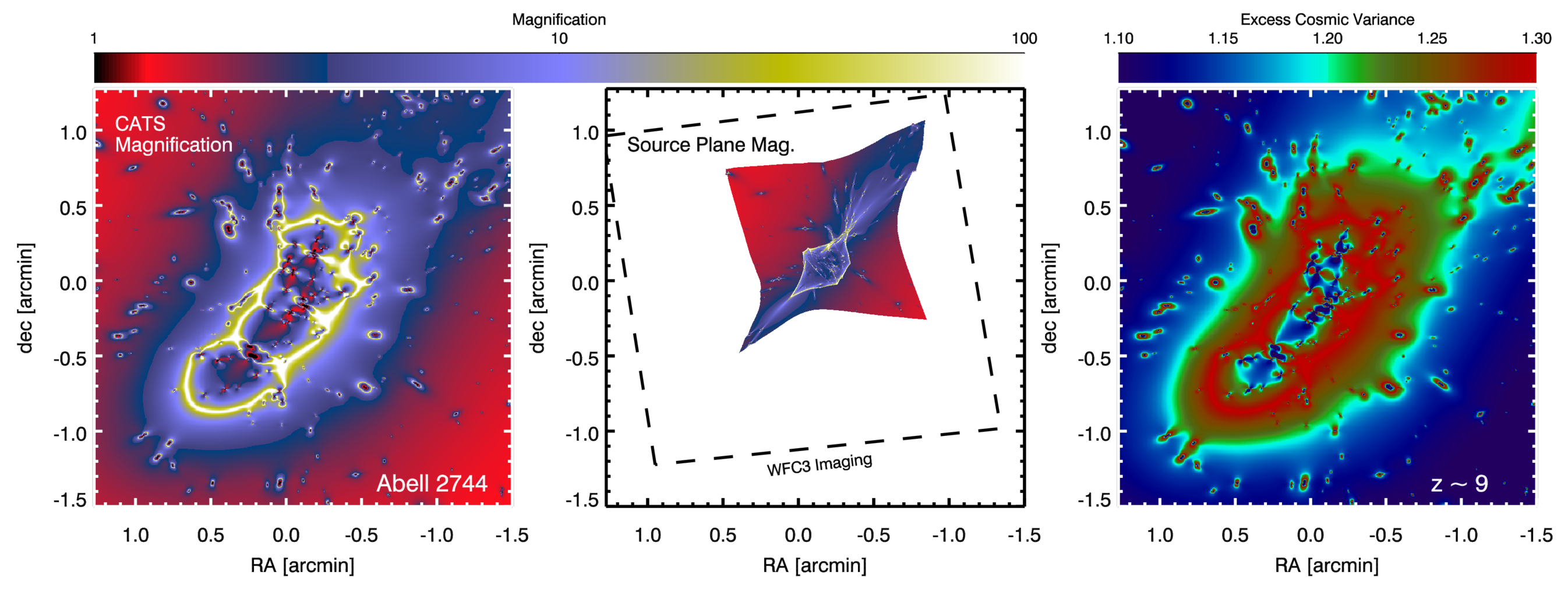
Applying the methods presented in Sections 2 and 3 to the Frontier Fields (FF) requires using magnification and deflection maps of individual cluster lenses to reconstruct the effective area of the HST survey in the source plane. Figure 1 illustrates our methodology applied to A2744. We use the Clusters As TelescopeS (CATS) lens models presented in Richard et al. (2014) that provide a map of the spatially-dependent magnification (left panel of Figure 1, shown for the $z\sim 9$ model). The public Richard et al. (2014) models also include a matrix of deflections that allows for a reconstruction of a source plane magnification map. We use the HST WFC3 weight map from the public FF data (Program ID 13495; PI Lotz, Co-PI Mountain) to determine the area of A2744 covered by WFC3 imaging, and then reconstruct the source plane magnification map of this region (our method is similar to that presented by Coe et al. 2014 and produces similar results to their Figure 5). The reconstructed source plane magnification map is shown in the middle panel of Figure 1, and enables us to compute the area $A(\mu>\mu_{i})$ that defines the intrinsic luminosity-dependent window function used in Equation 2 to calculate the sample variance. The connection between magnification, source plane effective area, and CV can then be used to produce a “cosmic variance map” of A2744. The right panel of Figure 1 shows the estimated excess CV in the A2744 field relative to a blank field of the same imaging area, as a function of the local magnification. The CV in A2744 is estimated to be $10-30\%$ higher than in an equivalent blank field survey, assuming a constant bias population. Applying the same methodology to the other FF lens models suggests similarly increased uncertainties.

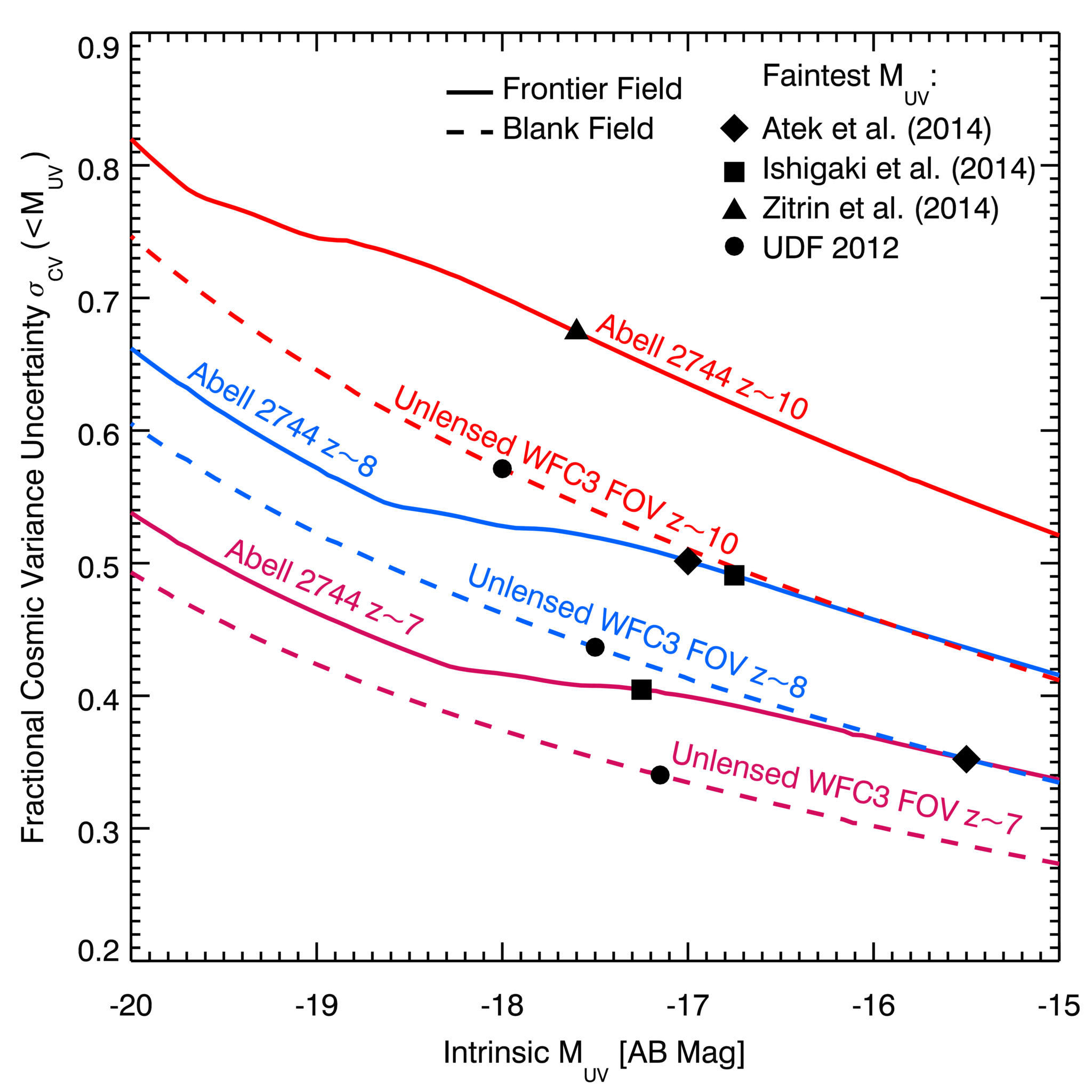
The luminosity-dependent CV uncertainty of the A2744 lens galaxy population can be estimated as a function of intrinsic source flux. Figure 2 shows the fractional CV uncertainty of the high-redshift galaxy population statistics for unlensed surveys the size of a single WFC3 field-of-view (dashed lines) and for a lensed population behind A2744 (solid lines), calculated assuming the redshift-dependent luminosity function parameters presented in Bouwens et al. (2014). The CV uncertainty is computed for $z\sim 7$ (magenta), $z\sim 8$ (blue), and $z\sim 10$ (red) populations. We have additionally indicated the CV estimates for the UDF 2012 survey (Ellis et al., 2013; Schenker et al., 2013; McLure et al., 2013), the Atek et al. (2014b) and Ishigaki et al. (2014) A2744 samples, and the Zitrin et al. (2014) $z\sim 10$ object identified in the A2744 data. The A2744 samples have CV uncertainties comparable to blank field surveys with depths $\sim 2$ magnitudes brighter. Since the CV of the lensed fields depends mostly on the source plane effective area as a function of magnification, Figure 2 should provide a useful CV estimate for any FF high-redshift sample.

HST Frontier Fields (FF) observations began in Cycle 21, and the program data has already identified distant galaxies behind A2744 (Atek et al., 2014a, b; Zheng et al., 2014; Zitrin et al., 2014; Oesch et al., 2014). Several FF analyses have referred to the blank-field calculations of Trenti & Stiavelli (2008) to determine the CV of A2744 samples (e.g., Atek et al., 2014a; Coe et al., 2014; Yue et al., 2014), but this model (and that discussed by Robertson 2010b) underestimates the CV uncertainty of gravitationally lensed populations. Zheng et al. (2014) comment on the possibility of an increased CV for their sample owing to lensing but provide no estimates. The new calculations presented in this Letter account for the increased CV in the FF relative to blank fields owing to the reduced effective volume of lensed surveys.¹¹1During the publication process, Atek et al. (2014b) was revised to reflect our CV estimates.

Understanding the CV of the FF samples is critical for interpreting highly-magnified faint objects in the broader context of the cosmic reionization process. The robust identification of a handful of extremely faint $z\sim 7-8$ objects in the FF could substantially improve the determination of the faint-end slope of the high-$z$ luminosity function, as indicated by the sample of Atek et al. (2014b) that reaches down to $M_{UV}\sim-15$. The ionizing photon luminosity density provided by high-$z$ galaxies identified above the limiting magnitude of the UDF ($M_{UV}\sim-17$ at $z\sim 7$) does not appear sufficient to reionize the universe fully by $z\sim 6$ under standard assumptions for the escape fraction and ionizing photon production per unit UV luminosity (Robertson et al., 2013). We infer that yet fainter galaxies must provide a significant contribution to the UV luminosity density, and therefore our understanding of the role of star-forming galaxies in reionization depends critically on uncertainties in the faint-end slope of the UV LF determination (Bolton & Haehnelt, 2007; Robertson et al., 2010, 2013; Kuhlen & Faucher-Giguère, 2012). Among the most precise determinations of the LF faint-end slope $\alpha$ at $z\sim 7,8$ that fully accounts for the CV uncertainty of these faint, distant galaxy samples was provided by Schenker et al. (2013) using the UDF and CANDELS Deep data, who found $\alpha(z\sim 7)=-1.87^{+0.18}_{-0.17}$ and $\alpha(z\sim 8)=-1.94^{+0.21}_{-0.24}$ (see also McLure et al., 2013). Similar faint-end slopes and uncertainties have been measured independently (Oesch et al., 2012; Bouwens et al., 2014) including using the A2744 sample (Atek et al., 2014b). As the lensed samples probe further down the luminosity function with highly magnified objects, abundance matching suggests that the clustering bias of the galaxy population is expected to decrease faster than the reduced source plane effective volume causes the rms density fluctuations to increase. Reaching substantially fainter galaxies therefore improves the CV statistics.

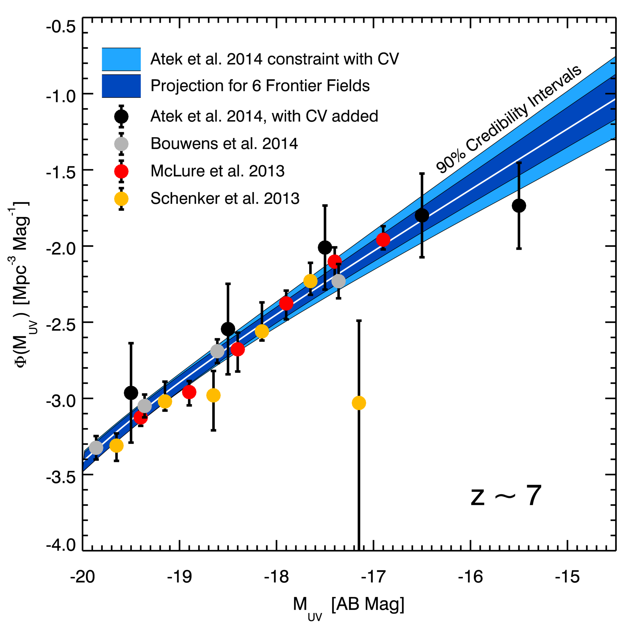
With an estimated CV uncertainty for the A2744 sample, we can revisit the analysis presented by Atek et al. (2014b) accounting for CV and estimate the additional constraints that might be provided by the complete FF program assuming A2744 is representative. Figure 3 shows the multi-field luminosity function data from Schenker et al. (2013), McLure et al. (2013), and Bouwens et al. (2014), and the A2744 data from Atek et al. (2014b). We have increased the uncertainties of the A2744 luminosity function data by adding the luminosity-dependent CV uncertainty shown in Figure 2 in quadrature with the errors reported by Atek et al. (2014b). Performing Bayesian parameter estimation based on the Multinest sampling algorithm (Feroz et al., 2009) and the Bouwens et al. (2014) and Atek et al. (2014b) data, we constrain the 90% credibility interval for the $z\sim 7$ luminosity function as shown in Figure 3 (light blue area). Assuming our best-fit luminosity function parameters ($\phi_{\star}=3.28\times 10^{-4}~\mathrm{Mpc}^{-3}~\mathrm{Mag}^{-1}$, $M_{\star}=-20.79$, $\alpha=-1.99$) are accurate and A2744 is a representative lens, we then perform Monte Carlo realizations of the galaxy population in five additional FF including the expected CV. Repeating our parameter estimation on these bootstrapped models of the complete six-cluster FF program (including the Bouwens et al. 2014 data as before) we find that the 90% credibility interval on the luminosity function shrinks considerably (dark area in Figure 3). Importantly, this result suggests the complete FF program can provide critical information on the cosmic production rate of Lyman continuum photons by faint galaxies required to reionize the intergalactic medium by $z\sim 6$. We forecast that the complete FF program may reduce the uncertainty on the $z\sim 7$ faint-end slope to $\sigma_{\alpha}\lesssim 0.05$ and the fractional uncertainty in UV luminosity density extrapolated to $M_{UV}=-13$ by a factor of $2\times$ to $\sim 30\%$. The FF program may therefore help resolve whether star-forming galaxies were primarily responsible for completing the cosmic reionization process. The FF may also help constrain the evolution of the global star formation history at $z\sim 7-10$, but such an analysis will require a careful treatment of the CV of lensed populations.

We conclude by highlighting some features and limitations of our CV calculations for the FF program. The computation of the source plane area requires the use of a lens model and, while we use the CATS model of A2744 presented by Richard et al. (2014), picking a different public lens model (e.g., Johnson et al., 2014) can change the source plane effective volume by $>10\%$ (see Figure 5 of Coe et al., 2014). The range of source plane effective areas among the FF clusters is about a factor of 3, with A2744 being among the largest. The typical CV uncertainty of the high-redshift samples in the other FF will be comparable to or slightly greater than that of A2744, provided the intrinsic luminosity distributions of the sources are comparable.

The typical CV uncertainty is of order unity, suggesting that our quasilinear model may underestimate the true sample variance. The highly-lensed volumes are extremely small ($V\lesssim 100$Mpc³ for magnifications $\mu\geq 10$; see, e.g., Figure 5 of Coe et al. 2014), so nonlinear halo bias may complicate the clustering statistics (e.g., Fernandez et al., 2012; Kitaura et al., 2014). Precise applications of the FF samples for constraining the luminosity function or high-redshift star formation rate density may therefore require more detailed modeling.

The large clustering bias of early galaxy populations and small volumes probed by distant surveys make cosmic variance an important source of uncertainty for high-redshift observations. These concerns are intensified for strongly-lensed surveys like the Frontier Fields, as the amplification of source fluxes through gravitational magnification comes at the cost of a decreased effective survey volume. We present the first estimates of the cosmic variance uncertainty associated with distant galaxy populations identified in the Frontier Fields, using Abell 2744 as a representative example. By our estimates, the cosmic variance uncertainty increases from $\sim 35\%$ for the redshift $z\sim 7$ sample of Atek et al. (2014a, b) to $\gtrsim 65\%$ for inferences drawn from the $z\sim 10$ object examined by Zitrin et al. (2014) and Oesch et al. (2014). While these cosmic variance uncertainties are amplified relative to blank-field surveys like the Ultra Deep Field (Beckwith et al., 2006; Ellis et al., 2013), they provide an independent sample to improve luminosity function and star formation rate density estimates at high-redshift, provided that their statistical properties are handled appropriately (McLeod et al., 2014).

References

- Atek et al. (2014a) Atek, H., et al. 2014a, ApJ, 786, 60
- Atek et al. (2014b) —. 2014b, ArXiv e-prints
- Beckwith et al. (2006) Beckwith, S. V. W., et al. 2006, AJ, 132, 1729
- Bolton & Haehnelt (2007) Bolton, J. S., & Haehnelt, M. G. 2007, MNRAS, 382, 325
- Bouwens et al. (2011) Bouwens, R. J., et al. 2011, ApJ, 737, 90
- Bouwens et al. (2014) —. 2014, ArXiv e-prints
- Bradley et al. (2014) Bradley, L. D., et al. 2014, ApJ, 792, 76
- Coe et al. (2014) Coe, D., Bradley, L., & Zitrin, A. 2014, ArXiv e-prints
- Coe et al. (2013) Coe, D., et al. 2013, ApJ, 762, 32
- Conroy et al. (2006) Conroy, C., Wechsler, R. H., & Kravtsov, A. V. 2006, ApJ, 647, 201
- Curtis-Lake et al. (2014) Curtis-Lake, E., et al. 2014, ArXiv e-prints
- Dunlop et al. (2013) Dunlop, J. S., et al. 2013, MNRAS, 432, 3520
- Eisenstein & Hu (1998) Eisenstein, D. J., & Hu, W. 1998, ApJ, 496, 605
- Ellis et al. (2013) Ellis, R. S., et al. 2013, ApJ, 763, L7
- Fernandez et al. (2012) Fernandez, E. R., Iliev, I. T., Komatsu, E., & Shapiro, P. R. 2012, ApJ, 750, 20
- Feroz et al. (2009) Feroz, F., Hobson, M. P., & Bridges, M. 2009, MNRAS, 398, 1601
- Finkelstein et al. (2012) Finkelstein, S. L., et al. 2012, ApJ, 758, 93
- Grogin et al. (2011) Grogin, N. A., et al. 2011, ApJS, 197, 35
- Illingworth et al. (2013) Illingworth, G. D., et al. 2013, ApJS, 209, 6
- Ishigaki et al. (2014) Ishigaki, M., Kawamata, R., Ouchi, M., Oguri, M., Shimasaku, K., & Ono, Y. 2014, ArXiv e-prints
- Johnson et al. (2014) Johnson, T. L., Sharon, K., Bayliss, M. B., Gladders, M. D., Coe, D., & Ebeling, H. 2014, ArXiv e-prints
- Kitaura et al. (2014) Kitaura, F.-S., Yepes, G., & Prada, F. 2014, MNRAS, 439, L21
- Koekemoer et al. (2013) Koekemoer, A. M., et al. 2013, ApJS, 209, 3
- Koekemoer et al. (2011) —. 2011, ApJS, 197, 36
- Kravtsov et al. (2004) Kravtsov, A. V., Berlind, A. A., Wechsler, R. H., Klypin, A. A., Gottlöber, S., Allgood, B., & Primack, J. R. 2004, ApJ, 609, 35
- Kuhlen & Faucher-Giguère (2012) Kuhlen, M., & Faucher-Giguère, C.-A. 2012, MNRAS, 423, 862
- McLeod et al. (2014) McLeod, D., Dunlop, J. S., & McLure, R. 2014, in preparation
- McLure et al. (2013) McLure, R. J., et al. 2013, MNRAS, 432, 2696
- McLure et al. (2010) McLure, R. J., Dunlop, J. S., Cirasuolo, M., Koekemoer, A. M., Sabbi, E., Stark, D. P., Targett, T. A., & Ellis, R. S. 2010, MNRAS, 403, 960
- Oesch et al. (2010) Oesch, P. A., et al. 2010, ApJ, 709, L16
- Oesch et al. (2014) Oesch, P. A., Bouwens, R. J., Illingworth, G. D., Franx, M., Ammons, S. M., van Dokkum, P. G., Trenti, M., & Labbe, I. 2014, ArXiv e-prints
- Oesch et al. (2012) Oesch, P. A., et al. 2012, ApJ, 759, 135
- Ono et al. (2013) Ono, Y., et al. 2013, ApJ, 777, 155
- Planck Collaboration et al. (2013) Planck Collaboration, et al. 2013, ArXiv e-prints
- Postman et al. (2012) Postman, M., et al. 2012, ApJS, 199, 25
- Richard et al. (2014) Richard, J., et al. 2014, MNRAS, 444, 268
- Robertson (2010a) Robertson, B. E. 2010a, ApJ, 716, L229
- Robertson (2010b) —. 2010b, ApJ, 713, 1266
- Robertson et al. (2010) Robertson, B. E., Ellis, R. S., Dunlop, J. S., McLure, R. J., & Stark, D. P. 2010, Nature, 468, 49
- Robertson et al. (2013) Robertson, B. E., et al. 2013, ApJ, 768, 71
- Schenker et al. (2013) Schenker, M. A., et al. 2013, ApJ, 768, 196
- Tinker et al. (2008) Tinker, J., Kravtsov, A. V., Klypin, A., Abazajian, K., Warren, M., Yepes, G., Gottlöber, S., & Holz, D. E. 2008, ApJ, 688, 709
- Tinker et al. (2010) Tinker, J. L., Robertson, B. E., Kravtsov, A. V., Klypin, A., Warren, M. S., Yepes, G., & Gottlöber, S. 2010, ApJ, 724, 878
- Trenti & Stiavelli (2008) Trenti, M., & Stiavelli, M. 2008, ApJ, 676, 767
- Yue et al. (2014) Yue, B., Ferrara, A., Vanzella, E., & Salvaterra, R. 2014, MNRAS, 443, L20
- Zheng et al. (2012) Zheng, W., et al. 2012, Nature, 489, 406
- Zheng et al. (2014) —. 2014, ArXiv e-prints
- Zitrin et al. (2014) Zitrin, A., et al. 2014, ArXiv e-prints