Accumulation of elastic strain toward crustal fracture in magnetized neutron stars

We consider the dynamical force balance between pressure, gravity, and the Lorentz force. The MHD equilibrium is described as follows:

where $\Phi_{\rm g}$ is the gravitational potential including the centrifugal terms. The third term has a magnitude $\sim 10^{-7}(B/10^{14}{\rm G})^{2}$ times smaller than those of the first and second terms. Deviation owing to the Lorentz force is small enough to be treated as a perturbation on a background equilibrium.

We limit our consideration to an axially symmetric configuration for the magnetic-field configuration. The poloidal and toroidal components of the magnetic field are expressed by two functions $\Psi$ and $S$, respectively, as follows:

where $\varpi=r\sin\theta$ is the cylindrical radius, and ${\bf{e}}_{\phi}$ is the azimuthal unit-vector in $(r,\theta,\phi)$ coordinates. When the equilibrium is barotropic, i.e., the constant surfaces of $\rho$ and $P$ are parallel, the azimuthal current $j_{\phi}$ is described in the form

where the current function $S$ should be a function of $\Psi$, and $K$ is another function of $\Psi$. For the axially symmetric barotropic equilibrium, acceleration due to the Lorentz force, which is abbreviated as ${{\bf{a}}}\equiv(c\rho)^{-1}{{\bf{j}}}\times{{\bf{B}}}$, is given by

The force balance (1) is described by gradient terms of scalar functions.

The magnetic function $\Psi$ is obtained by solving the Ampére–Biot–Savart law with the source term (Equation (3)) after the functional forms $S(\Psi)$ and $K(\Psi)$ are specified. For simplicity, we assume that $K$ is a linear function of $\Psi$, $K=K_{0}\Psi$, and $S=0$ in Equation (3). The poloidal magnetic field is purely dipolar and is given by $\Psi=g(r)\sin^{2}\theta$. The radial function $g$ is solved with appropriate boundary conditions: in a vacuum at the surface $R$, and $g=0$ at the core-crust interface $r_{c}$. The latter refers to the magnetic field expelled from the core. For the case where the field penetrates into the core, $g$ smoothly connects to the interior solution at $r_{c}$. We normalize the radial function by the dipole field strength $B_{0}$ at the surface, $g(R)=B_{0}R^{2}/2$.

The magnetic geometry discussed above is a simple initial model to examine the magnetic field evolution. However, purely poloidal magnetic field configurations are unstable according to an energy principle (Tayler, 1973; Markey & Tayler, 1973; Wright, 1973) and numerical MHD simulation (Braithwaite & Nordlund, 2006; Braithwaite, 2009; Lander & Jones, 2011a, b; Mitchell et al., 2015). Dynamical simulations revealed that the final state after a few Alfvén-wave crossing times is a twisted-torus configuration, in which the poloidal and toroidal components of comparable field strengths are tangled. Moreover, recent three-dimensional simulation shows very asymmetric equilibrium (Becerra et al., 2022). These studies are concerned with the configuration in an entire star. The information relevant to our study corresponds to the magnetic field in a thin outer layer; therefore, the present understanding is quite incomplete. For example, the ratio of toroidal to poloidal components decreases near the surface, because the toroidal field should vanish outside the exterior. However, the ratio in the crust located near the surface is uncertain, almost zero or in the order of unity, although both components are comparable in magnitude inside the star. Initially, a simple magnetic field configuration is used in this paper, but it is necessary to improve the configuration.

We discuss the non-barotropic equilibrium of the magnetic field. From Equation (1), the acceleration owing to the Lorentz force satisfies

The acceleration ${{\bf{a}}}$ is no longer described by the gradient of a scalar, but may be generalized as

where $\alpha$ and $\beta$ are functions of $r$ and $\theta$, and ${{\bf{\nabla}}}\times{{\bf{a}}}={{\bf{\nabla}}}\alpha\times{{\bf{\nabla}}}\beta\neq 0$ is assumed. Owing to almost arbitrary functions $\alpha$ and $\beta$, the constraint on the electric current, and hence to the magnetic-field configuration, is relaxed in the non-barotropic case. Non-barotropicity has been studied in magnetic deformation (Mastrano et al., 2011, 2013, 2015). Barotropic (Haskell et al., 2008; Kojima et al., 2021b) and non-barotropic models are significantly different. (Mastrano et al., 2011, 2013, 2015) up to approximately one order of magnitude in the resulting ellipticity. The effect is important; however, the treatment remains unclear. Therefore, we introduce the models of ${{\bf{\nabla}}}\times{{\bf{a}}}$ to study non-barotropicity in Section 4.

Our consideration is limited to the inner crust of a neutron star, where the mass density ranges from $\rho_{c}=1.4\times 10^{14}$ g cm^-3 at the core–crust boundary $r_{c}$ to the neutron-drip density $\rho_{1}=4\times 10^{11}$ g cm^-3 at $R=12$ km. We ignore the outer crust compared to “ocean” and treat the exterior region of $r>R$ as the vacuum. The crust thickness $\Delta r\equiv R-r_{c}$ is assumed to be $\Delta r/R=0.05$, $\Delta r=0.6$ km.

The Lorentz force ${{\bf{j}}}\times{{\bf{B}}}$ due to the magnetic-field evolution is not fixed in a secular timescale. The evolution in the crust is governed by the induction equation

where $n_{\rm e}$ is the electron-number density, and $\sigma$ is the electric conductivity. The first term in Equation (7) represents the Hall drift, and the Hall timescale $\tau_{\rm H}$ is estimated as follows:

where the electron-number density $n_{\rm ec}$ at the core–crust boundary, crust thickness $\Delta r$, and dipole field strength $B_{0}$ at the surface are used. This timescale is shorter than that of the Ohmic decay, which is the second term in Equation (7) in the strong-magnetic-field regime.

The Hall-Ohmic evolution was numerically simulated in the Hall timescale Pons & Geppert (2007); Kojima & Kisaka (2012); Viganò et al. (2013); Gourgouliatos et al. (2013); Gourgouliatos & Cumming (2014); Viganò et al. (2021) for axially symmetric models. Recently, the calculation has been extended to 3D models Wood & Hollerbach (2015); Viganò et al. (2019); De Grandis et al. (2020); Gourgouliatos et al. (2020); Igoshev et al. (2021), revealing some of the effects ignored in the 2D models. Here, our calculation is limited to the early phase of the evolution in a simpler axial-symmetric model. We consider only the Hall drift term in Equation (7) and rewrite the equation as follows:

where

In Equation (10), ${\hat{\chi}}$ is a dimensionless function, which represents an inverse of the electron fraction. The electron-number density is obtained from the proton fraction of the equilibrium nucleus in ”cold catalyzed matter,” i.e., it is determined in the ground state at $T=0$ K. The data given by Douchin & Haensel (2001) is approximately fitted by a smooth function:

where ${\hat{\rho}}\equiv\rho/\rho_{c}.$ The spatial-density profile of a neutron star in $r_{c}\leq r\leq R$ is approximated as follows (Lander & Gourgouliatos, 2019):

The radial derivative $d{\hat{\chi}}/dr=(d{\hat{\chi}}/d\rho)(d\rho/dr)$ sharply changes, owing to an abrupt decrease in the density near the surface; however, ${\hat{\chi}}$ is a smoothly varying function of $\mathcal{O}(1)$. This functional behavior, which originates from the stellar-density profile that is inherent in neutron stars, is crucial in our numerical calculation. Different fitting formulae are discussed for different equation of state in Pearson et al. (2018); however, the difference in ${\hat{\chi}}$ is not significant in our analysis.

We consider the early phase of the evolution in the axially symmetric equilibrium model, in which $a_{\phi}=0$. From Equation (9) at $t=0$, we obtain that ${\partial B_{\phi}}/{\partial t}\neq 0$, but ${\partial B_{r}}/{\partial t}={\partial B_{\theta}}/{\partial t}=0$. The azimuthal component $B_{\phi}$ changes linearly with time $t$, whereas the poloidal components change with $t^{2}$. We limit our consideration to the lowest order of $t$ only and ignore the change in the poloidal magnetic field. The early phase of the toroidal magnetic field may be approximated as

where $\delta S$ is a function of $r$ and $\theta$. Because it is associated with $\delta B_{\phi}$, the poloidal current changes; thus, the Lorentz force $\delta{{\bf{f}}}=c^{-1}(\delta{{\bf{j}}}\times{{\bf{B}}}+{{\bf{j}}}\times\delta{{\bf{B}}})$ also changes. We observe that the non-zero component is $\delta f_{\phi}$ because ${{\bf{j}}}_{p}=B_{\phi}=0$ at $t=0$, and we explicitly write

We assume that the solid crust elastically acts against the force $\delta f_{\phi}$. The change is so slow that the elastic evolution is quasi-stationary. The acceleration $\partial^{2}\xi_{i}/\partial t^{2}$ of the elastic displacement vector $\xi_{i}$ is dismissed; thus, the elastic force is balanced with the change in the Lorentz force, i.e., when the gravity and pressure in Equation (1) is assumed to be fixed. The elastic force is expressed by the trace-free strain tensor $\sigma_{ij}$ and a shear modulus $\mu$; therefore, the force balance is

where incompressible motion ${\nabla}_{k}\xi^{k}=0$ is assumed. Alternatively, the equivalent form is

The relevant component induced by $\delta f_{\phi}$ is the azimuthal displacement $\xi_{\phi}$ only, and the shear tensors that are determined by it are

The shear modulus $\mu$ increases with density, and it may be approximated as a linear function of $\rho$, which is overall fitted to the results of a detailed calculation reported in a previous study (see Figure 43 in Chamel & Haensel, 2008).

where $\mu_{c}=10^{30}~{}{\rm erg~{}cm}^{-3}$ at the core–crust interface. The shear speed $v_{s}$ in Equation (19) is constant through the crust:

To solve Equation (15), we use an expansion method with the Legendre polynomials $P_{l}(\cos\theta)$ and radial functions $k_{l}(r)$, $a_{l}(r)$ as follows:

The displacement $\xi_{\phi}$ is decoupled with respect to the index $l$, owing to spherical symmetry, i.e., $\mu(r)$. Equation (15) is reduced to a set of ordinary differential equations for $k_{l}$ (Kojima et al., 2022):

where a prime ^′ denotes a derivative with respect to $r$. The boundary conditions for the radial functions $k_{l}$ are given by the force-balance across the surfaces at $r_{c}$ and $R$. That is, the shear-stress tensor $\sigma_{r\phi}$ vanishes because other stresses for the fluid and magnetic field are assumed to be continuous. Explicitly, we have $k_{l}^{\prime}=0$ both at $r_{c}$ and $R$. Note that a mode with $l=1$ is special in Equation (23), and $k_{1}$ is simply obtained by integrating $a_{1}$ with respect to $r$.

The shear stress increases homologously with time, i.e., the spatial profile of the shear force is unchanged, but the magnitude increases with time. The numerical calculation provides the maximum shear stress $\sigma_{\rm{max}}$ with respect to $(r,\theta)$ in the crust as follows:

The maximum is determined using a ratio of the shear speed $v_{s}$ in Equation (20) to the Alfvén speed $v_{a}$ in Equation (25). Elastic equilibrium is possible, only when the shear strain satisfies a particular criterion. We adopt the following (the Mises criterion) to determine the elastic limit:

where $\sigma_{c}$ is a number $\sigma_{c}\approx 10^{-2}-10^{-1}$ (Horowitz & Kadau, 2009; Caplan et al., 2018; Baiko & Chugunov, 2018).

Thus, the period of the elastic response is limited by the constraint $\sigma_{c}$:

The breakup time $t_{*}$ becomes short, i.e., a few years for magnetars with $B_{0}=10^{15}$G. This is in agreement with the recurrent time of the activity in magnetars. However, the timescale exceeds 1 Myr for most neutron stars with $B<10^{13}{\rm G}$. Moreover, other evolution effects are important, and present results are not applicable.

The stored elastic energy is obtained by numerically integrating over the entire crust:

where we have used $R^{3}$ instead of $R^{2}{\Delta{r}}$ to normalize the crustal volume because ${\Delta{r}}/R=0.05$ is fixed. The elastic energy $E_{\rm ela}$ increases up to $\approx 10^{41}$ erg at the breakup time $t_{*}$.

The magnetic energy $\Delta E_{\rm mag}$ is also obtained by

Here, the shear speed appears in $\Delta E_{\rm mag}$ because the breakup time $t_{*}$ in Equation (29) is used instead of $\tau_{\rm H}$. The magnetic energy $\Delta E_{\rm mag}$ at $t_{*}$ is $\Delta E_{\rm mag}\approx 2\times 10^{43}(B_{0}/10^{14}{\rm G})^{-2}$ erg. However, it is considerably smaller than the poloidal magnetic energy $E_{\rm mag,p}$, which is numerically calculated as $E_{\rm mag,p}=3.8B_{0}^{2}R^{3}\approx 4\times 10^{46}(B_{0}/10^{14}{\rm G})^{2}$ erg. Note that total magnetic energy is conserved by the Hall evolution. Therefore, the same amount of polar magnetic energy decreases. However, we ignored the change in the poloidal component and its energy, which are proportional to $t^{2}$.

The ratio of Equations (31) and (32) is

where $\mu_{c}$ and $B_{0}^{2}$ are eliminated using $v_{s}$ and $v_{a}$. The ratio is proportional to $B_{0}^{2}$; thus, $\Delta E_{\rm mag}$ decreases in more strongly magnetized neutron stars. From the viewpoint of the energy flow from the poloidal component, the breakup energy $\Delta E_{\rm ela}\approx 10^{41}$ at the terminal is fixed, but the $\Delta E_{\rm mag}$ stored in the middle depends on the Hall drift speed. The elastic energy is efficiently accumulated through toroidal magnetic energy with an increase in $B_{0}$; $\Delta E_{\rm ela}>\Delta E_{\rm mag}$ for $B_{0}>6.7\times 10^{14}$ G.

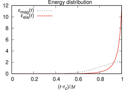
Figure 1 shows spatial-energy densities $\varepsilon_{\rm ela}(r)$ and $\varepsilon_{\rm mag}(r)$, with regard to $\Delta E_{\rm ela}$ and $\Delta E_{\rm mag}$ in the crust, respectively. They are normalized as $\int\varepsilon_{\rm ela}dr=\int\varepsilon_{\rm ela}dr=1$. Evidently, both energies are highly concentrated near the surface $r\approx R$. This property comes from the radial derivative of ${\hat{\chi}}$ in Equation (10). $d{\hat{\chi}}/dr=(d{\hat{\chi}}/d\rho)(d\rho/dr)$ is steep there even though ${\hat{\chi}}$ is $\mathcal{O}(1)$. The large value comes from $|d\rho/dr|$, i.e., a sharp decrease in density near the stellar surface, and it results in a smaller evolution timescale $\ll\tau_{\rm{H}}$ in Equation (29).

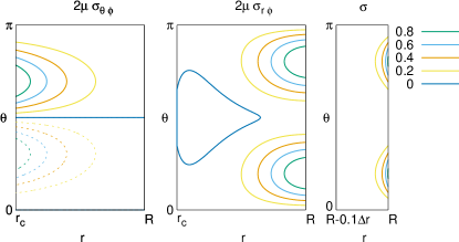
Shear stresses $\sigma_{\theta\phi}$ and $\sigma_{r\phi}$ are induced by the axial displacement $\xi_{\phi}$. A numerical calculation shows that the component $\sigma_{r\phi}$ is considerably larger than $\sigma_{\theta\phi}$; $(\sigma_{r\phi})_{\rm max}\sim 200(\sigma_{\theta\phi})_{\rm max}$. Figure 2 shows their spatial distribution using a contour map of $2\mu\sigma_{\theta\phi}$ and $2\mu\sigma_{r\phi}$ in the $r-\theta$ plain. The angular dependence of $\sigma_{\theta\phi}$ is $\sigma_{\theta\phi}\propto\sin^{2}\theta\cos\theta$, and it is anti-symmetric with respect to the equator ($\theta=\pi/2$). Moreover, $\sigma_{r\phi}$ is the sum of $P_{1,\theta}$ and $P_{3,\theta}$, and it is symmetric with respect to $\theta=\pi/2$. The magnitude $\sigma=(\sigma_{ij}\sigma^{ij}/2)^{1/2}$ is also shown in the right panel, and $\sigma$ is sharp near the surface, as expected from the sharp energy-density-distribution in Figure 1

We discuss the modification of the poloidal magnetic field at the core–crust boundary. Thus far, the magnetic field is expelled there. When the field is penetrated to the core, the function $g$ near the boundary and the constant $K_{0}$ in Equation (24) are changed. The former is unimportant because the function ${\hat{\chi}}^{\prime}$ is sharp near the surface, and this fact determines the result, as shown in Figures 1 and 2. The constant $K_{0}$ for the penetrated field is $4.1\times 10^{-2}$ times smaller than that for the expelled one. Consequently, the profile is almost unchanged, but the break time $t_{*}$ increases by a factor of 24 with the same dipole field strength.

We neglect the first term in Equation (9), and consider the magnetic-field evolution driven by the term ${{\bf{\nabla}}}\times{{\bf{a}}}$ (Equation (34)) only. Similar to the calculations in Section 3, a linearly growing shear–stress is obtained, owing to $\xi_{\phi}$. The period of the elastic response is limited by

where $n_{1}$ is a number of the order of $10^{-2}$, depending on the models, as listed in Table 1. Owing to our simple modeling, the comparison between the barotropic and non-barotropic models is uncomplicated; the Alfvén speed $v_{a}$ in Equation (29) is formally substituted by $N$ in Equation (36).

The elastic energy $\Delta E_{\rm ela}$ and toroidal magnetic energy $\Delta E_{\rm mag}$ stored inside the crust are also summarized as follows:

where $n_{2}\approx 6\times 10^{-4}$, and $n_{3}\approx 10^{-6}$, as listed in Table 1. The elastic energy $\Delta E_{\rm ela}$ does not depend on $N$; however, the timescale (36) does. The amount of elastic energy is unrelated to the detailed process, which affects the accumulation speed in the crust. At the breakup time, the elastic energy is $\Delta E_{\rm ela}=2\times 10^{44}-2\times 10^{45}$ erg. This energy is more than three orders of magnitude larger than the energy (31) considered in the previous section. The difference is made clear when considering the energy–density distribution.

Figure 3 shows the energy–density distribution in the crust. The difference in the toroidal magnetic energy clearly originates in the model choice; the energy density spreads more towards the interior for the ”in” model, whereas it spreads more towards the exterior for the ”out” model. Most of the elastic energy is localized near the inner core–crust boundary; however, the distribution in the ”out” model is shifted outwardly with the second peak ($\sim r_{c}+0.8{\Delta}r$) produced by the input model. The integrated elastic energy in the ”out” model becomes one order of magnitude smaller than that in the ”in” model.

The amount of elastic energy at the breakup clearly depends on the spatial distribution of the energy density because the shear modulus $\mu$ is a strongly decreasing function toward the surface. The elastic limit of the entire crust is typically determined using a condition to the shear $\sigma_{ij}$ near the surface. The total elastic energy $\sim\int\mu\sigma_{ij}\sigma^{ij}d^{3}x$ thereby decreases as $\sigma_{ij}\sigma^{ij}$ is localized towards the exterior. The breakup elastic energy $\Delta E_{\rm ela}\sim 10^{41}$ erg at $t_{*}$ in the previous section is an extreme case because the energy density is concentrated near the surface.

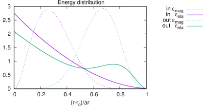
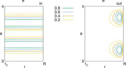
Figure 4 shows the magnitude of shear stress $\sigma$ inside the crust. The contours of $\sigma$ in the two models are different. We identified that the dominant component in the ”in” model (left panel) is $\sigma_{\theta\phi}$, which has an angular dependence that is described by $\sigma_{\theta\phi}\propto\sin^{2}\theta\cos\theta$. The maximum of $\sigma$ is given along a line $\cos\theta=\pm 1/\sqrt{3}~{}(\theta\sim 55^{\circ},125^{\circ})$. The component $\sigma_{r\phi}$ is dominant in the ”out” model (right panel). Sharp peaks are localized near the surface, similar to the right panel in Figure 2; however, the localization is not as pronounced as in Figure 2. The magnitude $\sigma$, which is important to determine the critical limit, is large near the surface.

In a more realistic situation, the solenoidal acceleration may fluctuate spatially. We consider the sum of multi-pole components $P_{l,\theta}$:

where $\lambda_{l}F_{n}$ is a radial function that is randomly selected from $\pm F_{1}$ or $\pm F_{3}$ depending on $l$. As discussed for Equation (26), the radial function $k_{l}$ in the azimuthal displacement $\xi_{\phi}$ is solved for the source term that originates from $\lambda_{l-1}F_{n}$ and $\lambda_{l+1}F_{n}$; thus, the amplitude $|k_{l}|$ fluctuates according to the randomness. We fix the overall constant $N$. Equation (39) is reduced to Equation (34) when $l_{\rm max}=2$. Moreover, higher $l$-modes, up to $l_{\rm max}=30$ with the power-law weight, are included. The power-law index is considerably steep; therefore, the dominant component is still described by $l=2$.

We calculated 20 models by randomly mixing $\lambda_{l}F_{n}$. The numerical results are summarized in the same forms as eqs. (36)–(38), and the numerical values $n_{i}~{}(i=1,2,3)$ in the breakup time and energies are listed in Table 1 according to the average, minimum, and maximum for the 20 models. These numerical values are of the same order as those by a single mode with $l=2$ because we include higher $l$-modes as the correction. Interestingly, the breakup time $t_{*}$ generally becomes shorter than that for a single mode with $l=2$ because the higher modes $l>3$ are cooperative.

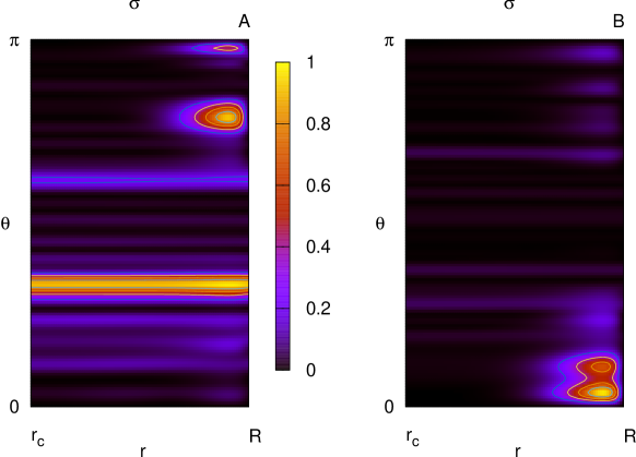
Figure 5 demonstrates the spatial distribution of the shear stress tensor. Two models are shown using contours of the magnitude of $\sigma$. In the left panel, the sub-critical regions are on a constant $\theta$ line with a sharp peak near the surface. In the other model (right panel), a peak is observed at $\theta=0$ near the surface. The angular position of the peak is different between the two models. As shown in Figure 4, the spatial pattern along a constant $\theta$ comes from the component $\sigma_{\theta\phi}$, whereas the sharp peak near the surface is due to $\sigma_{r\phi}$. The mixing of the two types of radial functions, $F_{1}$ and $F_{3}$, and angular functions $P_{l}$ with random phases and weights only complicates the spatial distribution of $\sigma$. A sharp peak is likely to be located near the surface. The outer part of the crust is always fragile; thus, the breakup time becomes shorter.

References

- Abbott et al. (2021a) Abbott, R., Abe, H., Acernese, F., et al. 2021a, ApJ, 921, 80, doi: 10.3847/1538-4357/ac17ea
- Abbott et al. (2021b) —. 2021b, ApJ, 913, L27, doi: 10.3847/2041-8213/abffcd
- Abbott et al. (2022) —. 2022, arXiv e-prints, arXiv:2204.04523. https://arxiv.org/abs/2204.04523
- Alpar et al. (1984) Alpar, M. A., Pines, D., Anderson, P. W., & Shaham, J. 1984, ApJ, 276, 325, doi: 10.1086/161616
- Anderson & Itoh (1975) Anderson, P. W., & Itoh, N. 1975, Nature, 256, 25, doi: 10.1038/256025a0
- Baiko & Chugunov (2018) Baiko, D. A., & Chugunov, A. I. 2018, MNRAS, 480, 5511, doi: 10.1093/mnras/sty2259
- Basu et al. (2022) Basu, A., Shaw, B., Antonopoulou, D., et al. 2022, MNRAS, 510, 4049, doi: 10.1093/mnras/stab3336
- Becerra et al. (2022) Becerra, L., Reisenegger, A., Valdivia, J. A., & Gusakov, M. E. 2022, MNRAS, 511, 732, doi: 10.1093/mnras/stac102
- Bochenek et al. (2020) Bochenek, C. D., Ravi, V., Belov, K. V., et al. 2020, Nature, 587, 59, doi: 10.1038/s41586-020-2872-x
- Braithwaite (2009) Braithwaite, J. 2009, MNRAS, 397, 763, doi: 10.1111/j.1365-2966.2008.14034.x
- Braithwaite & Nordlund (2006) Braithwaite, J., & Nordlund, Å. 2006, A&A, 450, 1077, doi: 10.1051/0004-6361:20041980
- Caplan et al. (2018) Caplan, M. E., Schneider, A. S., & Horowitz, C. J. 2018, Phys. Rev. Lett., 121, 132701, doi: 10.1103/PhysRevLett.121.132701
- Chamel & Haensel (2008) Chamel, N., & Haensel, P. 2008, Living Reviews in Relativity, 11, 10, doi: 10.12942/lrr-2008-10
- CHIME/FRB Collaboration et al. (2020) CHIME/FRB Collaboration, Andersen, B. C., Bandura, K. M., et al. 2020, Nature, 587, 54, doi: 10.1038/s41586-020-2863-y
- De Grandis et al. (2020) De Grandis, D., Turolla, R., Wood, T. S., et al. 2020, ApJ, 903, 40, doi: 10.3847/1538-4357/abb6f9
- Dehman et al. (2020) Dehman, C., Viganò, D., Rea, N., et al. 2020, ApJ, 902, L32, doi: 10.3847/2041-8213/abbda9
- Dib et al. (2008) Dib, R., Kaspi, V. M., & Gavriil, F. P. 2008, ApJ, 673, 1044, doi: 10.1086/524653
- Douchin & Haensel (2001) Douchin, F., & Haensel, P. 2001, A&A, 380, 151, doi: 10.1051/0004-6361:20011402
- Espinoza et al. (2011) Espinoza, C. M., Lyne, A. G., Stappers, B. W., & Kramer, M. 2011, MNRAS, 414, 1679, doi: 10.1111/j.1365-2966.2011.18503.x
- Esposito et al. (2021) Esposito, P., Rea, N., & Israel, G. L. 2021, in Astrophysics and Space Science Library, Vol. 461, Astrophysics and Space Science Library, ed. T. M. Belloni, M. Méndez, & C. Zhang, 97–142, doi: 10.1007/978-3-662-62110-3_3
- Franco et al. (2000) Franco, L. M., Link, B., & Epstein, R. I. 2000, ApJ, 543, 987, doi: 10.1086/317121
- Giliberti et al. (2020) Giliberti, E., Cambiotti, G., Antonelli, M., & Pizzochero, P. M. 2020, MNRAS, 491, 1064, doi: 10.1093/mnras/stz3099
- Gittins et al. (2021) Gittins, F., Andersson, N., & Jones, D. I. 2021, MNRAS, 500, 5570, doi: 10.1093/mnras/staa3635
- Gourgouliatos (2022) Gourgouliatos, K. N. 2022, arXiv e-prints, arXiv:2202.06662. https://arxiv.org/abs/2202.06662
- Gourgouliatos & Cumming (2014) Gourgouliatos, K. N., & Cumming, A. 2014, MNRAS, 438, 1618, doi: 10.1093/mnras/stt2300
- Gourgouliatos et al. (2013) Gourgouliatos, K. N., Cumming, A., Reisenegger, A., et al. 2013, MNRAS, 434, 2480, doi: 10.1093/mnras/stt1195
- Gourgouliatos et al. (2020) Gourgouliatos, K. N., Hollerbach, R., & Igoshev, A. P. 2020, MNRAS, 495, 1692, doi: 10.1093/mnras/staa1295
- Gourgouliatos & Lander (2021) Gourgouliatos, K. N., & Lander, S. K. 2021, MNRAS, 506, 3578, doi: 10.1093/mnras/stab1869
- Haskell et al. (2006) Haskell, B., Jones, D. I., & Andersson, N. 2006, MNRAS, 373, 1423, doi: 10.1111/j.1365-2966.2006.10998.x
- Haskell et al. (2008) Haskell, B., Samuelsson, L., Glampedakis, K., & Andersson, N. 2008, MNRAS, 385, 531, doi: 10.1111/j.1365-2966.2008.12861.x
- Horowitz & Kadau (2009) Horowitz, C. J., & Kadau, K. 2009, Phys. Rev. Lett., 102, 191102, doi: 10.1103/PhysRevLett.102.191102
- Igoshev et al. (2021) Igoshev, A. P., Gourgouliatos, K. N., Hollerbach, R., & Wood, T. S. 2021, ApJ, 909, 101, doi: 10.3847/1538-4357/abde3e
- Kaspi & Beloborodov (2017) Kaspi, V. M., & Beloborodov, A. M. 2017, ARA&A, 55, 261, doi: 10.1146/annurev-astro-081915-023329
- Kojima & Kisaka (2012) Kojima, Y., & Kisaka, S. 2012, MNRAS, 421, 2722, doi: 10.1111/j.1365-2966.2012.20509.x
- Kojima et al. (2021a) Kojima, Y., Kisaka, S., & Fujisawa, K. 2021a, MNRAS, 506, 3936, doi: 10.1093/mnras/stab1848
- Kojima et al. (2021b) —. 2021b, MNRAS, 502, 2097, doi: 10.1093/mnras/staa3489
- Kojima et al. (2022) —. 2022, MNRAS, 511, 480, doi: 10.1093/mnras/stac036
- Kojima & Suzuki (2020) Kojima, Y., & Suzuki, K. 2020, MNRAS, 494, 3790, doi: 10.1093/mnras/staa1045
- Lander et al. (2015) Lander, S. K., Andersson, N., Antonopoulou, D., & Watts, A. L. 2015, MNRAS, 449, 2047, doi: 10.1093/mnras/stv432
- Lander & Gourgouliatos (2019) Lander, S. K., & Gourgouliatos, K. N. 2019, MNRAS, 486, 4130, doi: 10.1093/mnras/stz1042
- Lander & Jones (2011a) Lander, S. K., & Jones, D. I. 2011a, MNRAS, 412, 1394, doi: 10.1111/j.1365-2966.2010.17998.x
- Lander & Jones (2011b) —. 2011b, MNRAS, 412, 1730, doi: 10.1111/j.1365-2966.2010.18009.x
- Li et al. (2022) Li, X., Ge, M., Lin, L., et al. 2022, ApJ, 931, 56, doi: 10.3847/1538-4357/ac6587
- Markey & Tayler (1973) Markey, P., & Tayler, R. J. 1973, MNRAS, 163, 77, doi: 10.1093/mnras/163.1.77
- Mastrano et al. (2013) Mastrano, A., Lasky, P. D., & Melatos, A. 2013, MNRAS, 434, 1658, doi: 10.1093/mnras/stt1131
- Mastrano et al. (2011) Mastrano, A., Melatos, A., Reisenegger, A., & Akgün, T. 2011, MNRAS, 417, 2288, doi: 10.1111/j.1365-2966.2011.19410.x
- Mastrano et al. (2015) Mastrano, A., Suvorov, A. G., & Melatos, A. 2015, MNRAS, 447, 3475, doi: 10.1093/mnras/stu2671
- Mereghetti et al. (2020) Mereghetti, S., Savchenko, V., Ferrigno, C., et al. 2020, ApJ, 898, L29, doi: 10.3847/2041-8213/aba2cf
- Mitchell et al. (2015) Mitchell, J. P., Braithwaite, J., Reisenegger, A., et al. 2015, MNRAS, 447, 1213, doi: 10.1093/mnras/stu2514
- Payne & Melatos (2004) Payne, D. J. B., & Melatos, A. 2004, MNRAS, 351, 569, doi: 10.1111/j.1365-2966.2004.07798.x
- Pearson et al. (2018) Pearson, J. M., Chamel, N., Potekhin, A. Y., et al. 2018, MNRAS, 481, 2994, doi: 10.1093/mnras/sty2413
- Pons & Geppert (2007) Pons, J. A., & Geppert, U. 2007, A&A, 470, 303, doi: 10.1051/0004-6361:20077456
- Pons & Perna (2011) Pons, J. A., & Perna, R. 2011, ApJ, 741, 123, doi: 10.1088/0004-637X/741/2/123
- Rencoret et al. (2021) Rencoret, J. A., Aguilera-Gómez, C., & Reisenegger, A. 2021, A&A, 654, A47, doi: 10.1051/0004-6361/202141499
- Rheinhardt & Geppert (2002) Rheinhardt, M., & Geppert, U. 2002, Phys. Rev. Lett., 88, 101103, doi: 10.1103/PhysRevLett.88.101103
- Suvorov & Kokkotas (2019) Suvorov, A. G., & Kokkotas, K. D. 2019, MNRAS, 488, 5887, doi: 10.1093/mnras/stz2052
- Tayler (1973) Tayler, R. J. 1973, MNRAS, 161, 365, doi: 10.1093/mnras/161.4.365
- Turolla et al. (2015) Turolla, R., Zane, S., & Watts, A. L. 2015, Reports on Progress in Physics, 78, 116901, doi: 10.1088/0034-4885/78/11/116901
- Ushomirsky et al. (2000) Ushomirsky, G., Cutler, C., & Bildsten, L. 2000, MNRAS, 319, 902, doi: 10.1046/j.1365-8711.2000.03938.x
- Viganò et al. (2021) Viganò, D., Garcia-Garcia, A., Pons, J. A., Dehman, C., & Graber, V. 2021, Computer Physics Communications, 265, 108001, doi: 10.1016/j.cpc.2021.108001
- Viganò et al. (2013) Viganò, D., Rea, N., Pons, J. A., et al. 2013, MNRAS, 434, 123, doi: 10.1093/mnras/stt1008
- Viganò et al. (2019) Viganò, D., Martínez-Gómez, D., Pons, J. A., et al. 2019, Computer Physics Communications, 237, 168, doi: 10.1016/j.cpc.2018.11.022
- Wadiasingh & Chirenti (2020) Wadiasingh, Z., & Chirenti, C. 2020, ApJ, 903, L38, doi: 10.3847/2041-8213/abc562
- Wood & Hollerbach (2015) Wood, T. S., & Hollerbach, R. 2015, Phys. Rev. Lett., 114, 191101, doi: 10.1103/PhysRevLett.114.191101
- Wood et al. (2014) Wood, T. S., Hollerbach, R., & Lyutikov, M. 2014, Physics of Plasmas, 21, 052110, doi: 10.1063/1.4879810
- Wright (1973) Wright, G. A. E. 1973, MNRAS, 162, 339, doi: 10.1093/mnras/162.4.339
- Younes et al. (2022) Younes, G., Lander, S. K., Baring, M. G., et al. 2022, ApJ, 924, L27, doi: 10.3847/2041-8213/ac4700