Accuracy and Fairness Trade-offs in Machine Learning:
A Stochastic Multi-Objective Approach
Abstract
In the application of machine learning to real-life decision-making systems, e.g., credit scoring and criminal justice, the prediction outcomes might discriminate against people with sensitive attributes, leading to unfairness. The commonly used strategy in fair machine learning is to include fairness as a constraint or a penalization term in the minimization of the prediction loss, which ultimately limits the information given to decision-makers. In this paper, we introduce a new approach to handle fairness by formulating a stochastic multi-objective optimization problem for which the corresponding Pareto fronts uniquely and comprehensively define the accuracy-fairness trade-offs. We have then applied a stochastic approximation-type method to efficiently obtain well-spread and accurate Pareto fronts, and by doing so we can handle training data arriving in a streaming way.
1 Introduction
Machine learning (ML) plays an increasingly significant role in data-driven decision making, e.g., credit scoring, college admission, hiring decisions, and criminal justice. As the learning models became more and more sophisticated, concern regarding fairness started receiving more and more attention. In 2014, the Obama Administration’s Big Data Report (Podesta et al., 2014) claimed that discrimination against individuals and groups might be the “inadvertent outcome of the way big data technologies are structured and used”. Two years later, a White House report (2016) on the challenges of big data emphasized the necessity of promoting fairness and called for equal opportunity in insurance, education, employment, and other sectors.
In supervised machine learning, training samples consist of pairs of feature vectors (containing a number of features that are descriptive of each instance) and target values/labels. One tries to determine an accurate predictor, seen as a function mapping feature vectors into target labels. Such a predictor is typically characterized by a number of parameters, and the process of identifying the optimal parameters is called training or learning. The trained predictor can then be used to predict labels for unlabeled instances.
If a ML predictor does inequitably treat people from different groups defined by sensitive or protected attributes, such as gender, race, country, or disability, we say that such a predictor is unfair. The sources of unfairness in supervised ML are twofold. Firstly, the ML predictors are trained on data collected by humans (or automated agents developed by humans), which may contain inherent biases. Hence, by learning from biased or prejudiced targets, the prediction results obtained from standard learning processes can hardly be unbiased. Secondly, even if the targets are unbiased, the learning process may sacrifice fairness, as the main goal of ML is to make predictions as accurate as possible. In fact, previous research work (Pedreshi et al., 2008; Zemel et al., 2013) has showed that simply excluding sensitive attributes from features data (also called fairness through unawareness) does not help due to the fact that the sensitive attributes can be inferred from the nonsensitive ones.
Hence, a proper framework for evaluating and promoting fairness in ML becomes indispensable and relevant. Depending on when the fairness criteria are imposed, there are three categories of approaches proposed to handle fairness, namely pre-processing, in-training, and post-processing. Pre-processing approaches (Calmon et al., 2017; Zemel et al., 2013) modify the input data representation so that the prediction outcomes from any standard learning process become fair, while post-processing (Hardt et al., 2016; Pleiss et al., 2017) tries to adjust the results of a pre-trained predictor to increase fairness while maintaining the prediction accuracy as much as possible. Assuming that the sensitive attributes information are accessible in the training samples, most of in-training methods (Barocas & Selbst, 2016; Calders et al., 2009; Kamishima et al., 2011; Zafar et al., 2017b; Woodworth et al., 2017; Zafar et al., 2017a; Navon et al., 2021) enforce fairness during the training process either by directly imposing fairness constraints and solving constrained optimization problems or by adding penalization terms to the learning objective.
The approach proposed in our paper falls into the in-training category. We will however explicitly recognize the presence of at least two conflicting objectives in fair machine learning: (1) maximizing prediction accuracy; (2) maximizing fairness (w.r.t. certain sensitive attributes).
Multi-objective optimization methodology has been applied to various machine learning models to tackle conflicting objectives. In neural network training, a trade-off between accuracy and complexity were naturally formulated as a bi-objective problem and solved to get the Pareto front using evolutionary optimization methods (Yusiong & Naval, 2006; Kaoutar & Mohamed, 2017; Senhaji et al., 2017, 2020) or scalarization-based optimization methods (Kokshenev & Braga, 2008; Reiners et al., 2020). Similarly, two competing goals were constructed to minimize the training loss and minimize the model capacity in support vector machines (Bi, 2003; Igel, 2005) and decision trees (Kim, 2004). The obtained Pareto fronts supported down-streaming tasks like feature selection and model selection. Beyond that, conflicting objectives are found in multi-task learning (Sener & Koltun, 2018; Varghese & Mahmoud, 2020; Zhang & Yang, 2021) and data clustering (Handl & Knowles, 2004; Law et al., 2004). More multi-objective training frameworks were reviewed by (Jin, 2006; Braga et al., 2006; Jin & Sendhoff, 2008; Alexandropoulos et al., 2019). The conflict between accuracy and fairness is a new research topic in multi-objective machine learning. To the best of our knowledge, only a limited number of frameworks (Zafar et al., 2017a, b; Navon et al., 2021) were designed towards computing a substantial part of the entire trade-off curve.
1.1 Existing Fairness Criteria in Machine Learning
Fairness in machine learning basically requires that prediction outcomes do not disproportionally benefit people from majority and minority or historically advantageous and disadvantageous groups. In the literature of fair machine learning, several prevailing criteria for fairness include disparate impact (Barocas & Selbst, 2016) (also called demographic parity (Calders et al., 2009)), equalized odds (Hardt et al., 2016), and its special case of equal opportunity (Hardt et al., 2016), corresponding to different aspects of fairness requirements.
In this paper, we will focus on binary classification to present the formula for fairness criteria and the proposed accuracy and fairness trade-off framework, although they can all be easily generalized to other ML problems (such as regression or clustering). We point out that many real decision-making problems such as college admission, bank loan application, hiring decisions, etc. can be formulated into binary classification models.
Let denote feature vector, binary-valued sensitive attribute (for simplicity we focus on the case of a single binary sensitive attribute), and target label respectively. Consider a general predictor which could be a function of both and or only . The predictor is free of disparate impact (Barocas & Selbst, 2016) if the prediction outcome is statistically independent of the sensitive attribute, i.e., for ,
| (1) |
However, disparate impact could be unrealistic when one group is more likely to be classified as a positive class than others, an example being that women are more dominating in education and healthcare services than men (Kelly, 2020). As a result, disparate impact may never be aligned with a perfect predictor .
In terms of equalized odds (Hardt et al., 2016), the predictor is defined to be fair if it is independent of the sensitive attribute but conditioning on the true outcome , namely for ,
| (2) |
Under this definition, a perfectly accurate predictor can be possibly defined as a fair one, as the probabilities in (2) will always coincide when . Equal opportunity (Hardt et al., 2016), a relaxed version of equalized odds, requires that condition (2) holds for only positive outcome instances (), for example, students admitted to a college and candidates hired by a company.
1.2 Our Contribution
From the perspective of multi-objective optimization (MOO), most of the in-training methods in the literature (Barocas & Selbst, 2016; Calders et al., 2009; Kamishima et al., 2011; Woodworth et al., 2017; Zafar et al., 2017a, b) are based on the so-called a priori methodology, where the decision-making preference regarding an objective (the level of fairness) must be specified before optimizing the other (the accuracy). For instance, the constrained optimization problems proposed in (Zafar et al., 2017a, b) are to some extent nothing else than the –constraint method (Haimes, 1971) in MOO. Such procedures highly rely on the decision-maker’s advanced knowledge of the magnitude of fairness, which may vary from criterion to criterion and from dataset to dataset.
In order to better frame our discussion of accuracy vs fairness, let us introduce the general form of a multi-objective optimization problem
| (3) |
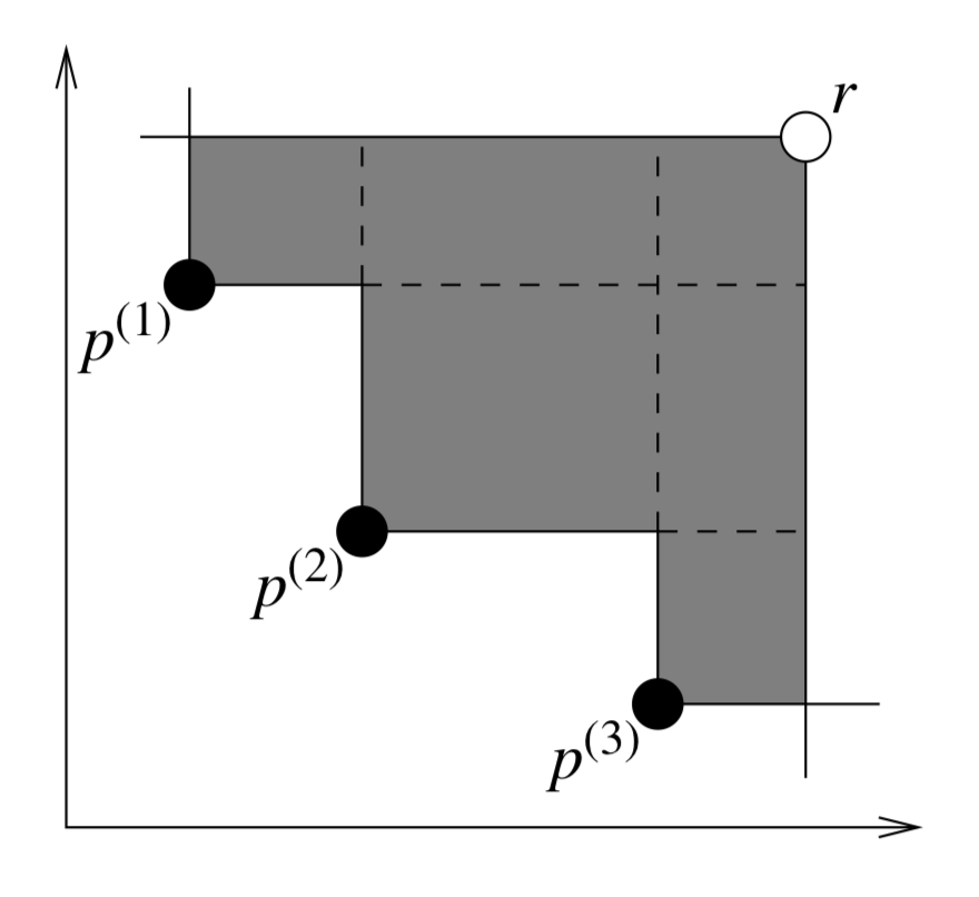
with objectives, and where . Usually, there is no single point optimizing all the objectives simultaneously. The notion of dominance is used to define optimality in MOO. A point (weakly) dominates if holds element-wise and additionally holds for at least one objective . A point is said to be (strictly) nondominated if it is not (weakly) dominated by any other point . An unambiguous way of considering the trade-offs among multiple objectives is given by the so-called Pareto front, which lies in the criteria space and is defined as the set of points of the form for all nondominated points . The concept of dominance is carried out from the decision space to the image one, and one can also say that (strictly) dominates when holds element-wise and holds for at least one . Finally, the terminology trade-off refers to compromising and balancing among the set of equally good nondominated solutions.
In this paper, instead of looking for a single predictor that satisfies certain fairness constraints, our goal is to directly construct a complete Pareto front between prediction accuracy and fairness, and thus to identify a set of predictors associated with different levels of fairness. We propose a stochastic multi-objective optimization framework, and aim at obtaining good approximations of true Pareto fronts. We summarize below the three main advantages of the proposed framework.
-
•
By applying an algorithm for stochastic multi-objective optimization (such as the Pareto front stochastic multi-gradient (PF-SMG) algorithm developed in (Liu & Vicente, 2021)), we are able to obtain well-spread and accurate Pareto fronts in a flexible and efficient way. The approach works for a variety of scenarios, including binary and categorical multi-valued sensitive attributes. It also handles multiple objectives simultaneously, such as multiple sensitive attributes and multiple fairness measures. Compared to the constrained optimization approaches, e.g., (Zafar et al., 2017a, b), our framework is proved to be computational efficient in constructing the whole Pareto fronts.
-
•
The proposed framework is quite general in the sense that it has no restriction on the type of predictors and works for any convex or nonconvex smooth objective functions. In fact, it can not only handle the fairness criteria mentioned in Section 1.1 based on covariance approximation, but also tackle other formula proposed in the literature, e.g., mutual information (Kamishima et al., 2012) and fairness as a risk measure (Williamson & Menon, 2019).
-
•
The PF-SMG algorithm falls into a Stochastic Approximation (SA) algorithmic approach, and thus it enables us to deal with the case where the training data is arriving on a streaming mode. By using such an SA framework, there is no need to reconstruct the Pareto front from scratch each time new data arrives. Instead, a Pareto front constructed based on consecutive arriving samples will eventually converge to the one corresponding to the overall true population.
By combining existing optimization methods and fairness concepts, this paper offers solutions to open ML fairness problems (non-convex measures, streaming data, multiple attributes, and multiple fairness measures). Our work provides a systematic and thorough trade-off approach from the viewpoint of stochastic multi-objective optimization for ML fairness.
The remainder of this paper is organized as follows. Our stochastic bi-objective formulation using disparate impact is suggested in Section 2. The PF-SMG algorithm, used to solve the multi-objective problems, is briefly introduced in Section 3 (more details in Appendix B). A number of numerical results for both synthetic and real data are presented in Section 4 to support our claims. Further exploring our line of thought, we introduce another stochastic bi-objective formulation, this time for trading-off accuracy vs equal opportunity (see Section 5), also reporting numerical results. In Section 6, we show how to handle multiple sensitive attributes and multiple fairness measures. For the purpose of getting more insight on the various trade-offs, two tri-objective problems are formulated and solved. Finally, a preliminary numerical experiment described in Section 7 will illustrate the applicability of our approach to streaming data. The paper is ended with some conclusions and prospects of future work in Section 8.
2 The Stochastic Bi-Objective Formulation Using Disparate Impact
Given that disparate impact is the most commonly used fairness criterion in the literature, we will first consider disparate impact in this section to present a stochastic bi-objective fairness and accuracy trade-off framework.
In our setting, the training samples consist of nonsensitive feature vectors , a binary sensitive attribute , and binary labels . Assume that we have access to samples from a given database. Let the binary predictor be a function of the parameters , and only learned from the nonsensitive feature .
Recall that the predictor is free of disparate impact if it satisfies equation (1). A general measurement of disparate impact, the so-called CV score (Calders & Verwer, 2010), is defined by the maximum gap between the probabilities of getting positive outcomes in different sensitive groups, i.e.,
| (4) |
The trade-offs between prediction accuracy and fairness can then be formulated as a general stochastic bi-objective optimization problem as follows
| (5) | ||||
| (6) |
where the first objective (5) is a composition function of a loss function and the prediction function , and the expectation is taken over the joint distribution of and .
The logistic regression model is one of the classical prediction models for binary classification problems. For purposes of binary classification, one aims at determining a linear classifier (noting ) in order to minimize a certain prediction loss. The data would be perfectly separated if when , and when for all pairs. The classical – loss function is given by , where . The logistic loss function is of the form , and is a smooth and convex version of the – loss. The first objective can then be approximated by the empirical logistic regression loss, i.e.,
| (7) |
based on training samples. A regularization term can be added to avoid over-fitting.
Dealing with the second objective (6) is challenging since it is nonsmooth and nonconvex. Hence, we make use of the decision boundary covariance proposed by (Zafar et al., 2017b) as a convex approximate measurement of disparate impact. Specifically, the CV score (4) can be approximated by the empirical covariance between the sensitive attributes and the hyperplane , i.e.,
where is the expected value of the sensitive attribute, and is an approximated value of using samples. The intuition behind this approximation is that the disparate impact (1) basically requires the predictor completely independent from the sensitive attribute.
Given that zero covariance is a necessary condition for independence, the second objective can be approximated as:
| (8) |
which, as we will see later in the paper, is monotonically increasing with disparate impact. We were thus able to construct a finite-sum bi-objective problem
| (9) |
where both functions are now convex and smooth.
3 The Stochastic Multi-Gradient Method and Its Pareto Front Version
Consider again a stochastic MOO of the same form as in (3), where some or all of the objectives involve uncertainty. Denote by a stochastic gradient of the -th objective function, where indicates the batch of samples used in the estimation. The stochastic multi-gradient (SMG) algorithm is described in Algorithm 1 (see Appendix A). It essentially takes a step along the stochastic multi-gradient which is a convex linear combination of , . The SMG method is a generalization of stochastic gradient (SG) to multiple objectives. It was first proposed by (Mercier et al., 2018) and further analyzed by (Liu & Vicente, 2021). In the latter paper it was proved that the SMG algorithm has the same convergence rates as SG (although now to a nondominated point), for both convex and strongly convex objectives. As we said before, when SMG reduces to SG. When and the ’s are deterministic, is the direction that is the most descent among all the functions (Fliege & Svaiter, 2000; Fliege et al., 2019).
Note that the two smooth objective functions (7) and (8) are both given in a finite-sum form, for which one can efficiently compute stochastic gradients using batches of samples.
To compute good approximations of the entire Pareto front in a single run, we use the Pareto Front SMG algorithm (PF-SMG) developed by (Liu & Vicente, 2021) (see Appendix B for an algorithm description). PF-SMG essentially maintains a list of nondominated points using SMG updates. It solves stochastic multi-objective problems in an a posteriori way, by determining Pareto fronts without predefining weights or adjusting levels of preferences. One starts with an initial list of randomly generated points ( in our experiments).
At each iteration of PF-SMG, we apply SMG multiple times at each point in the current list, and by doing so one obtains different final points due to stochasticity. At the end of each iteration, all the dominated points are removed to get a new list for the next iteration (see also Appendix B for an illustration of PF-SMG). The process can be stopped when either the number of nondominated points is greater than a certain budget (1,500 in our experiments) or when the total number of SMG iterates applied in any trajectory exceeds a certain budget (1,000 in our experiments). We refer to the paper (Liu & Vicente, 2021) for more details.
4 Numerical Results for Disparate Impact
4.1 Experiment setup
To numerically illustrate our approach based on the bi-objective formulation (9), we have used both the Adult Income dataset (Kohavi, 1996), which is available in the UCI Machine Learning Repository (Dua & Graff, 2017) and synthetic data (see Appendix D for the data generation).
There are several parameters to be tuned in PF-SMG for a better performance: (1) : number of times SMG is applied at each point in the current list; (2) : number of SMG iterations each time SMG is called; (3) : step size sequence; (4) : batch size sequences used in computing stochastic gradients for the two objectives. To control the rate of generated nondominated points, we remove nondominated points from regions where such points tend to grow too densely111Our implementation code is available at https://github.com/sul217/MOO_Fairness.. In our experiments, the parameters are selected using grid search. Specifically, for each combination of parameters, we run the PF-SMG using training data to get a set of nondominated solutions. The best parameter combination is chosen as the one with the most accurate predictor on the Pareto fronts which are evaluated using a set of validation samples.
Our approach is compared to the -constrained optimization model proposed in Zafar et al. (2017b, Equation (4)). From now on, we note their -constrained method as EPS-fair. It basically minimizes prediction loss subject to disparate impact being bounded above by a constant , i.e.,
Since the bi-objective problem (9) under investigation is convex, EPS-fair is able to compute a set of nondominated points by varying the value of . The implementation details of EPS-fair method can be found in (Zafar et al., 2017b). First, by solely minimizing prediction loss, a reasonable upper bound is obtained for disparate impact. Then, to obtain the Pareto front, a sequence of thresholds is evenly chosen from to such an upper bound, leading to a set of convex constrained optimization problems. The Sequential Least SQuares Programming (SLSQP) solver (Kraft, 1988) based on Quasi-Newton methods is then used for solving those problems. We found that 70-80% of the final points produced by this process were actually dominated ones, and we removed them for the purpose of analyzing results.
The cleaned up version of Adult Income dataset contains 45,222 samples. Each instance is characterized by 12 nonsensitive attributes (including age, education, marital status, and occupation), a binary sensitive attribute (gender), and a multi-valued sensitive attribute (race). The prediction target is to determine whether a person makes over 50K per year. Tables 2 and 2 in Appendix D show the detailed demographic composition of the dataset with respect to gender and race.
In the following experiments, we have randomly sampled 60% of the whole dataset for training, using 10% for validating and the remaining 30% instances as the testing dataset. The PF-SMG algorithm is applied using the training dataset, but all the Pareto fronts and the corresponding trade-off information will be presented using the testing dataset.
4.2 Numerical results
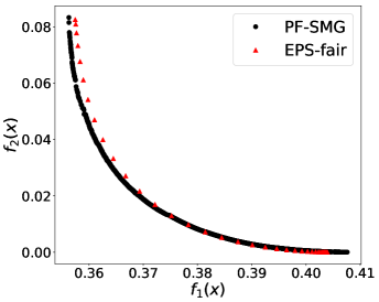
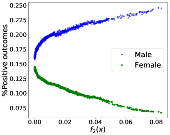
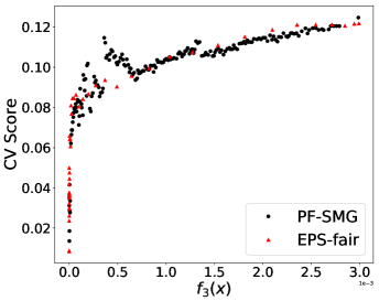
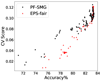
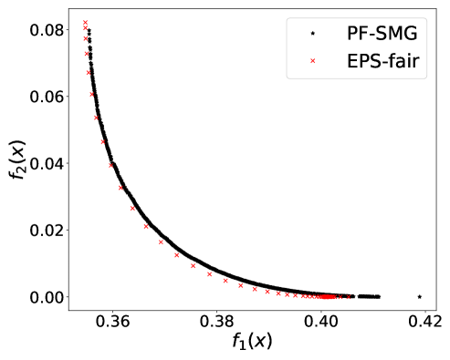
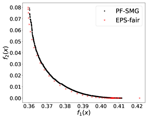
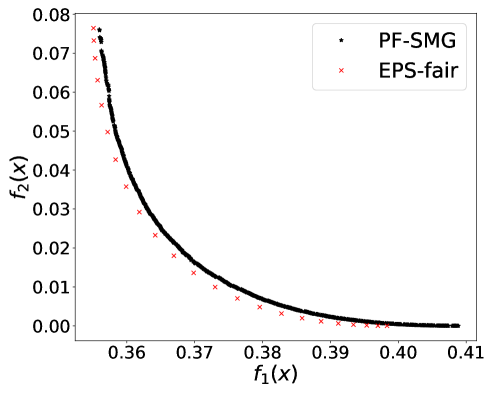
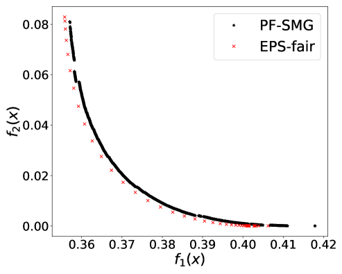
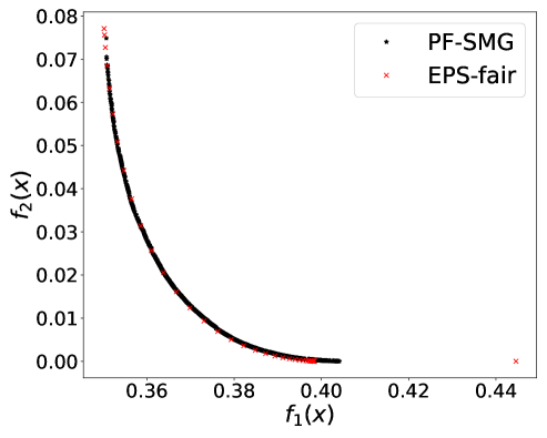
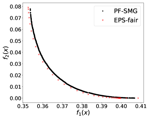
Performance in terms of trade-offs. Considering gender as the sensitive attribute, the obtained Pareto front by PF-SMG is plotted in Figure 1 (a), reconfirming the conflicting nature of the two objectives. Given a nondominated solution from Figure 1 (a), the probability of getting positive prediction for each sensitive group is approximated by the percentage of positive outcomes for the data samples, i.e., , where denotes the number of instances predicted as positive in group and is the number of instances in group . For conciseness, we will only compute the proportion of positive outcomes for analysis.
From Figure 1 (a), predictors of high accuracy are those of high disparate impact. It is then observed from Figure 1 (b) that as increases, the proportion of high income adults in females decreases, which means that the predictors of high accuracy are actually unfair for females. Figure 1 (c) we can conclude that the value of has positive correlation with CV score for this dataset. Figure 1 (d) implies that almost zero disparate impact can be achieved by reducing 1.5% of accuracy (the range of the x-axis is nearly 1.5%). To eliminate the impact of the fact that female is a minority in the dataset, we ran the algorithms for several sets of training samples with females and males. It turns out that the conflict is not alleviated at all. For comparison, the trade-off for the same training-testing split obtained by EPS-fair is also shown in Figures 1 (a), (c), and (d). More comparisons using different training-testing splits are given in Appendix E.1. It is clear that PF-SMG is more robust in capturing more complete and well-spread Pareto fronts.
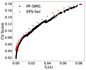
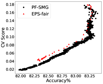
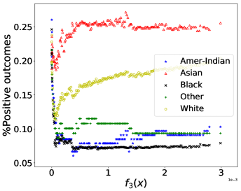
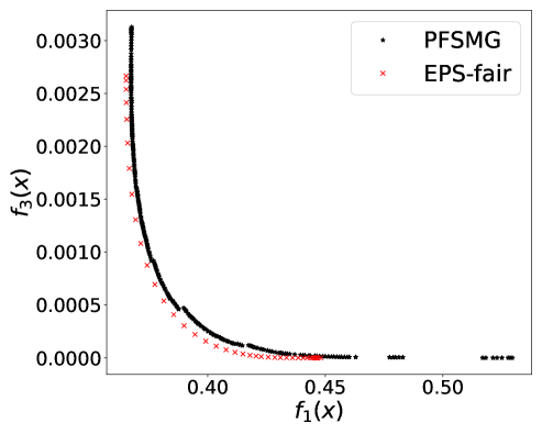
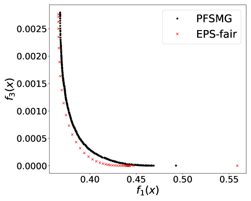
Dealing with multi-valued sensitive attribute race is more complicated. In general, if a multi-valued sensitive attribute has categorical values, we convert it to binary attributes denoted by . Note that the binary attribute indicates whether the original sensitive attribute has -th categorical value or not. The second objective is then modified as follows
| (10) |
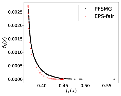
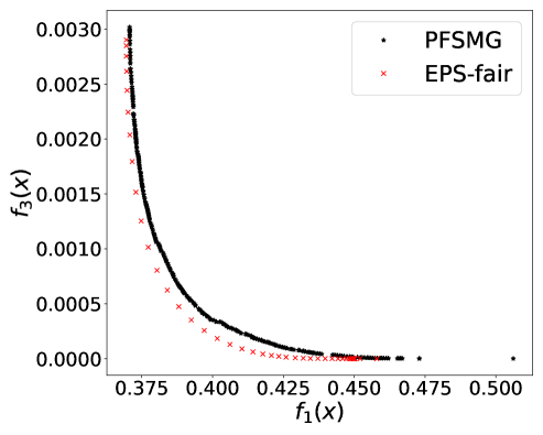
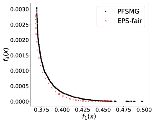
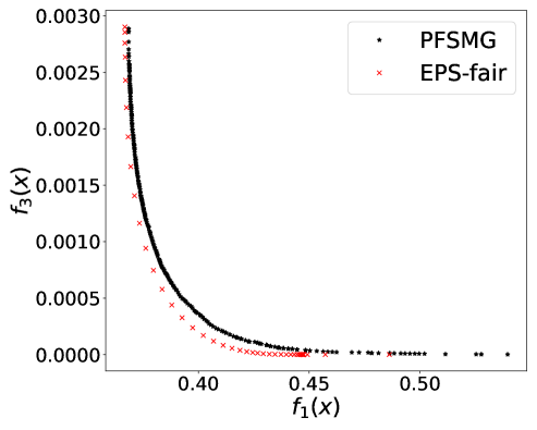
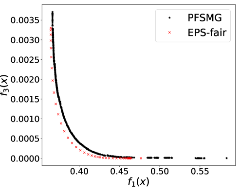
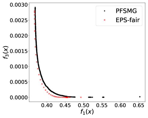
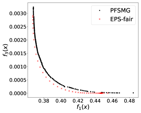
which is still a convex function. We have observed that the non-smoothness introduced by the max operator in (10) led to more discontinuity in the true trade-off curves, and besides stochastic gradient type methods are designed for smooth objective functions. We have thus approximated the max operator in (10) using . In our experiments, we set . Figure 2 (a) plots the obtained Pareto front of the bi-objective problem of . Figure 2 (b) implies that solely optimizing over prediction accuracy might result in unfair predictors for American-Indian, Black, and Other. Even though the individual percentage is not monotonically decreasing, the maximum gap of percentage is increasing while increases (Asian group excluded). Regardless of the noise, it is observed that the value of is increasing with CV score (Figure 2 (c)) and that the prediction accuracy and CV score have positive correlation (Figure 2 (d)). Note that CV score in this case was computed as the absolute difference between maximum and minimum proportions of positive outcomes among groups. The dominance effect of the Pareto fronts produced by PF-SMG over the ones produced by EPS-fair, seen in Figures 1 (a), (c), and (d), is now mixed in the ones of Figures 2 (a), (c), and (d). However, the spread and overall coverage of the fronts is better for PF-SMG in all the three plots. More results can be found in Appendix E.2.
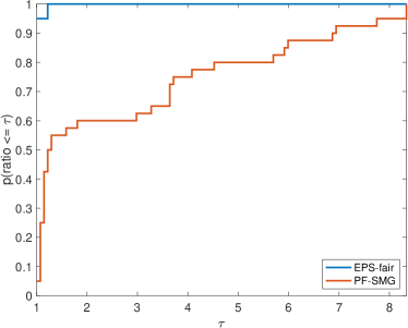
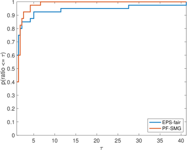
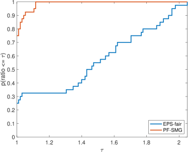
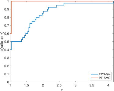
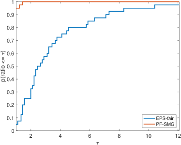
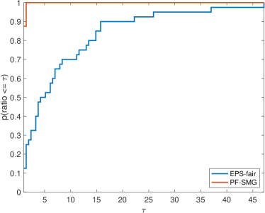
Performance in terms of efficiency and robustness. We systematically evaluated the performance of the two approaches by comparing CPU time per nondominated solution, number of gradient evaluations per nondominated solution, and the quality of Pareto fronts. Such a quality is measured by a formula called purity (which tries to evaluate how the fronts under analysis dominate each other) and two formulas for the spread of the fronts ( and , measuring how well the nondominated points on a Pareto front are distributed). Higher purity corresponds to higher accuracy, while smaller and indicate better spread. In addition, we also used hypervolume (Zitzler & Thiele, 1999), a performance measure combining purity and spread. The detailed formulas of the four measures are given in Appendix C.
We formed a set of 40 datasets with different random seeds: from synthetic data and from Adult income data ( binary and multi-valued problems). For EPS-fair, 1,500 and 100 different values of thresholds are evenly selected to form Pareto fronts for synthetic and real datasets respectively. To guarantee a fair comparison in terms of purity, spread, and hypervolume, the Pareto front generated by PF-SMG is down-sampled to matches the size of the corresponding Pareto front obtained by EPS-fair. The five performance profiles (see (Dolan & Moré, 2002)) are shown in Figure 3. The purity (see Figure 3 (a)) of the Pareto fronts produced by the EPS-fair method is slightly better than the one of those determined by PF-SMG. However, notice that PF-SMG produced better spread fronts than EPS-fair without compromising accuracy too much (see Figures 3 (b)–(c)). In fact, one can observe from Appendix E that the resulting Pareto fronts from PF-SMG are quite close to that from EPS-fair in the cases where the latter ones dominate the former ones. Further, Figure 3 (d) shows that PF-SMG wins against EPS-fair in terms of the combination of individual solution quality and objective space coverage. In addition, PF-SMG outperforms EPS-fair in terms of computational cost quantified by CPU time and gradient evaluations (see Figures 3 (e)–(f)).
5 Equal Opportunity
Recall that equal opportunity focuses on positive outcomes and requires the following for
When in the above equation, this condition essentially suggests equalized false negative rate (FNR) across different groups. Similarly, the case of corresponds to equalized true positive rate (TPR). Given that always holds, we will focus on the case where qualified candidates are falsely classified in a negative class by the predictor .
For simplicity, let , . The CV score associated with equal opportunity is now defined as follows
| (11) |
Since equalized FNR indicates statistical independence between sensitive attributes and instances that have positive targets but falsely predicted as negative, could thus be approximated (Zafar et al., 2017a) by
where . Here, excludes truly negative instances and implies wrong prediction. Similar to (8), the objective function for equalized FNR is given by
which is a nonconvex finite-sum function. (Note that as in (10) we have also smoothed here the min operator in .) Now, the finite-sum bi-objective problem becomes
| (12) |
Due to nonconvexity of the above problem, EPS-fair was not able to produce any reasonable trade-offs, and thus a comparison to our approach is not even applicable. The ProPublica COMPAS dataset (Larson et al., 2016b) contains features that are used by COMPAS algorithms (Larson et al., 2016a) for scoring defendants together with binary labels indicating whether or not a defendant recidivated within 2 years after the screening. For analysis, we take blacks and whites from the two-years-violent dataset (Larson et al., 2016b) and consider features including gender, age, number of prior offenses, and charge for which the person was arrested. For consistency with the word “opportunity”, we marked the case where a defendant is non-recidivist as the positive outcome. The demographic composition of the dataset is given in Table 3 in Appendix D. Due to shortage of data, we use the whole dataset for training and testing.
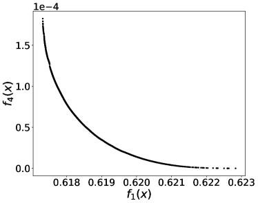
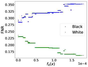
By applying PF-SMG to the bi-objective problem (12), we obtained the trade-off results in Figure 4. The conflicting nature of prediction loss and equalized FNR is confirmed by the Pareto front in Figure 4 (a). For each nondominated solution , we approximated FNR using samples by where is the number of instances satisfying all the conditions.
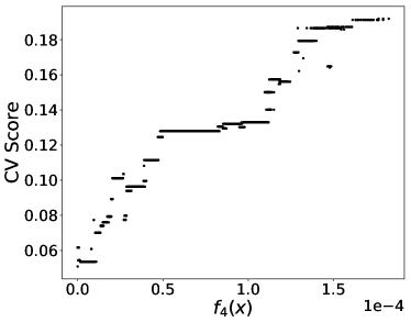
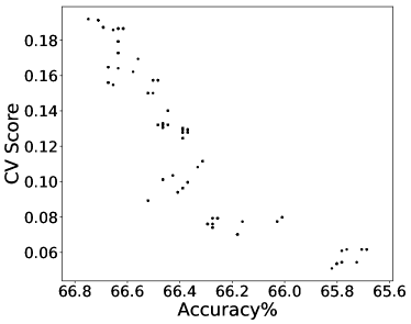
From the rightmost part of Figure 4 (b), we can draw a similar conclusion as in (Larson et al., 2016a) that black defendants (blue curve) who did not reoffend are accidentally predicted as recidivists twice as often as white defendants (green curve) when using the most accurate predictor obtained (i.e., versus ). However, the predictor associated with zero covariance (see the leftmost part) mitigates the situation to versus , although by definition the two rates should converge to the same point. This is potentially due to the fact that the covariance is not well approximated using a limited number of samples. In fact, the leftmost part of Figure 4 (c) shows that zero covariance does not correspond to zero . Finally, Figure 4 (d) provides a rough confirmation of positive correlation between CV score and prediction accuracy.
The results for equal opportunity presented in this section show the applicability of our multi-objective optimization framework when dealing with nonconvex fairness measures.
6 Handling Multiple Sensitive Attributes and Multiple Fairness Measures
A main advantage of handling fairness in machine learning through multi-objective optimization is the possibility of considering any number of criteria. In this section, we explore two possibilities, multiple sensitive attributes and multiple fairness measures.
6.1 Multiple Sensitive Attributes
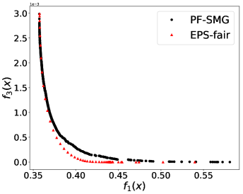
Let us see first how we can handle more than one sensitive attribute. One can consider a binary sensitive attribute (e.g. gender) and a multi-valued sensitive attribute (e.g. race), and formulate the following tri-objective problem
| (13) |
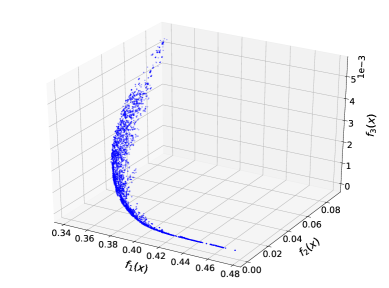
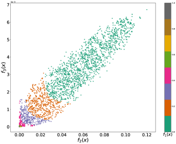
In our experiments, we use the Adult Income dataset and the splitting of training and testing samples of Subsection 4.2. A 3D Pareto front is plotted in Figure 5 (a) resulting from the application of PF-SMG to (13), with gender () and race () as the two sensitive attributes.
Figure 5 (b) depicts all the nondominated points projected onto the – objective space, where the points are colored according to the range of prediction loss. It is observed that there is no conflict between and . Although it could happen for other datasets, eliminating disparate impact with respect to gender does not hinder that with respect to race for this dataset. Intuitively, one could come up with a predictor where the proportions of positive predictions for female and male are equalized and the proportions of positive predictions for different races are equalized within the female and male groups separately, which would lead to zero disparate impact in terms of gender and race simultaneously.
6.2 Multiple Fairness Measures
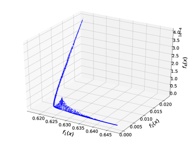
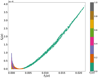
Now we see how to handle more than one fairness measure. As an example, we consider handling two fairness measures (disparate impact and equal opportunity) in the case of a binary sensitive attribute, and formulate the following tri-objective problem
| (14) |
In our experiments, we use the whole ProPublica COMPAS two-years-violent dataset (see Section 5) for both training and testing. Figure 5 (c) shows an approximated 3D Pareto front (resulting from the application of PF-SMG to (14)). By projecting all the obtained nondominated points onto the 2D – objective space, we have subplot (d), where the different colors indicate the different levels of prediction loss. From Figure 5 (d), one can easily find that an unique minimizer (in the gray area with lower prediction accuracy) exists for both and , and thus conclude that there is indeed no conflict between disparate impact and equal opportunity. In fact, by definition, the CV score (11) generalized to equal opportunity is a component of the CV score (4) measuring disparate impact. Therefore, in the darkgreen area where the accuracy is high enough, the values of the two fairness measures are aligned and increasing as the prediction accuracy increases. Interestingly, we have discovered a little Pareto front between and when the accuracy is limited in a certain medium level in between.
The proposed multi-objective approach works well in handling more than one sensitive attribute or multiple fairness measures. We point out that looking at Pareto fronts for three objectives helps us identifying the existence of conflicts among any subset of two objectives (compared to looking at Pareto fronts obtained just by solving the corresponding bi-objective problems). In the above experiments, by including , we were able to obtain additional helpful information in terms of decision-making reasoning.
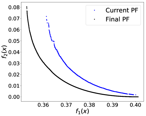
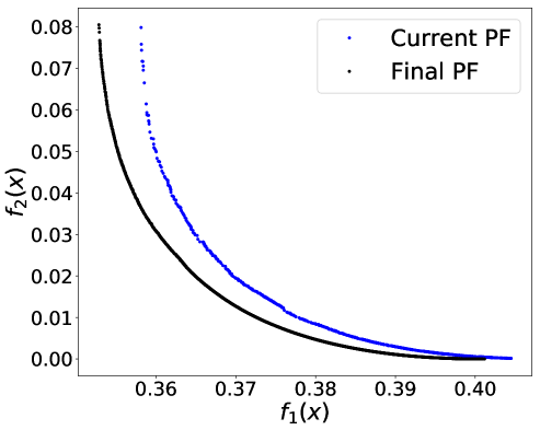
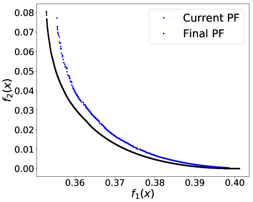
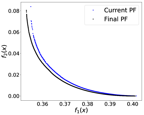
7 Streaming Data
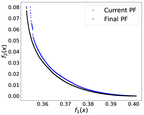
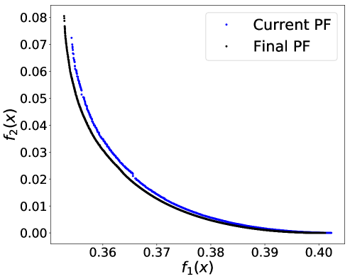
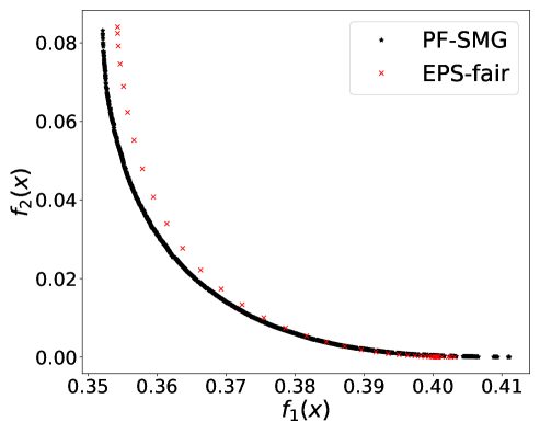
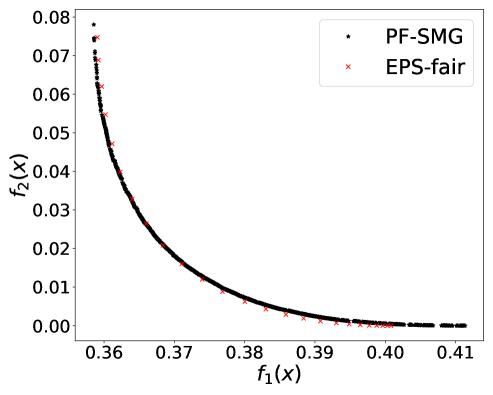
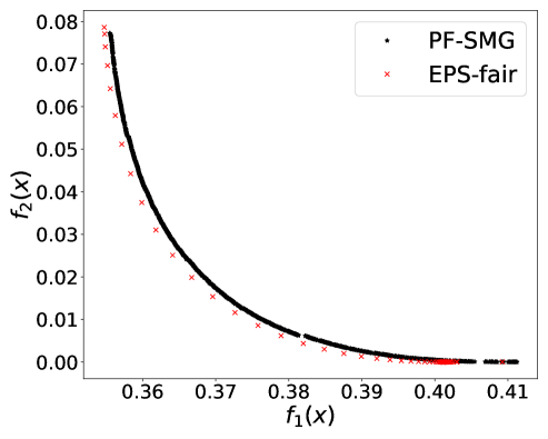
As we claimed in the Abstract and Introduction, another advantage of an SA-based approach like ours is its ability to handle streaming training data. We conducted a preliminary test using the Adult Income dataset and gender as the binary sensitive attribute. To simulate the streaming scenario, the whole dataset is split into batches of 2,000. The initial Pareto front is constructed by applying PF-SMG to one batch of 2,000 samples. Each time a new batch of samples is given, the Pareto front is then updated by selecting a number of nondominated points from the current Pareto front as the starting list for PF-SMG. Figures 10 given in Appendix E.3 shows how the successive Pareto fronts approach the final one computed for the whole dataset.
8 Concluding Remarks
We have proposed a novel stochastic multi-objective optimization framework to evaluate trade-offs between prediction accuracy and fairness for binary classification. A Stochastic Approximation (SA) algorithm like PF-SMG was proved to be computationally efficient to produce well-spread and sufficiently accurate Pareto fronts, when compared to the existing literature approach based on constraining the level of fairness. One can also handle both binary and categorical multi-valued sensitive attributes, but we improve over the literature since our approach can handle more than one sensitive attribute or different fairness measures simultaneously as well as streaming data.
The proposed framework can be generalized to accommodate different types of predictors and loss functions, including multi-class classification and regression. Moreover, our approach allows us to handle nonconvex approximations of disparate impact, equalized odds, or equal opportunity, two potential ones being mutual information (Kamishima et al., 2012) and fairness risk measures (Williamson & Menon, 2019).
References
- Alexandropoulos et al. (2019) Alexandropoulos, S.-A. N., Aridas, C. K., Kotsiantis, S. B., and Vrahatis, M. N. Multi-objective evolutionary optimization algorithms for machine learning: A recent survey. In Approximation and optimization, pp. 35–55. Springer, 2019.
- Barocas & Selbst (2016) Barocas, S. and Selbst, A. D. Big data’s disparate impact. California Law Review, 104:671, 2016.
- Bi (2003) Bi, J. Multi-objective programming in SVMs. In Proceedings of the 20th international conference on machine learning, pp. 35–42, 2003.
- Braga et al. (2006) Braga, A. P., Takahashi, R. H., Costa, M. A., and de Albuquerque Teixeira, R. Multi-objective algorithms for neural networks learning. In Multi-objective machine learning, pp. 151–171. Springer, 2006.
- Calders & Verwer (2010) Calders, T. and Verwer, S. Three naive Bayes approaches for discrimination-free classification. Data Mining and Knowledge Discovery, 21(2):277–292, 2010.
- Calders et al. (2009) Calders, T., Kamiran, F., and Pechenizkiy, M. Building classifiers with independency constraints. In 2009 IEEE International Conference on Data Mining Workshops, pp. 13–18. IEEE, 2009.
- Calmon et al. (2017) Calmon, F., Wei, D., Vinzamuri, B., Ramamurthy, K. N., and Varshney, K. R. Optimized pre-processing for discrimination prevention. In Advances in Neural Information Processing Systems, pp. 3992–4001, 2017.
- Custódio et al. (2011) Custódio, A. L. L., Madeira, J. A., Vaz, A. I. F., and Vicente, L. N. Direct multisearch for multiobjective optimization. SIAM J. Optim., 21(3):1109–1140, 2011.
- Deb et al. (2002) Deb, K., Pratap, A., Agarwal, S., and Meyarivan, T. A fast and elitist multiobjective genetic algorithm: NSGA-II. IEEE Transactions on Evolutionary Computation, 6(2):182–197, 2002.
- Dolan & Moré (2002) Dolan, E. D. and Moré, J. J. Benchmarking optimization software with performance profiles. Mathematical programming, 91(2):201–213, 2002.
- Dua & Graff (2017) Dua, D. and Graff, C. UCI Machine Learning Repository, 2017. URL http://archive.ics.uci.edu/ml.
- Fliege & Svaiter (2000) Fliege, J. and Svaiter, B. F. Steepest descent methods for multicriteria optimization. Math. Methods Oper. Res., 51(3):479–494, 2000.
- Fliege et al. (2019) Fliege, J., Vaz, A. I. F., and Vicente, L. N. Complexity of gradient descent for multiobjective optimization. Optimization Methods and Software, 34(5):949–959, 2019.
- Fonseca et al. (2006) Fonseca, C. M., Paquete, L., and López-Ibánez, M. An improved dimension-sweep algorithm for the hypervolume indicator. In 2006 IEEE international conference on evolutionary computation, pp. 1157–1163. IEEE, 2006.
- Haimes (1971) Haimes, Y. V. On a bicriterion formulation of the problems of integrated system identification and system optimization. IEEE Transactions on Systems, Man, and Cybernetics, 1(3):296–297, 1971.
- Handl & Knowles (2004) Handl, J. and Knowles, J. Evolutionary multiobjective clustering. In International Conference on Parallel Problem Solving from Nature, pp. 1081–1091. Springer, 2004.
- Hardt et al. (2016) Hardt, M., Price, E., and Srebro, N. Equality of opportunity in supervised learning. In Advances in neural information processing systems, pp. 3315–3323, 2016.
- Igel (2005) Igel, C. Multi-objective model selection for support vector machines. In International conference on evolutionary multi-criterion optimization, pp. 534–546. Springer, 2005.
- Jin (2006) Jin, Y. Multi-objective machine learning, volume 16. Springer Science & Business Media, 2006.
- Jin & Sendhoff (2008) Jin, Y. and Sendhoff, B. Pareto-based multiobjective machine learning: An overview and case studies. IEEE Transactions on Systems, Man, and Cybernetics, Part C (Applications and Reviews), 38(3):397–415, 2008.
- Kamishima et al. (2011) Kamishima, T., Akaho, S., and Sakuma, J. Fairness-aware learning through regularization approach. In 2011 IEEE 11th International Conference on Data Mining Workshops, pp. 643–650. IEEE, 2011.
- Kamishima et al. (2012) Kamishima, T., Akaho, S., Asoh, H., and Sakuma, J. Fairness-aware classifier with prejudice remover regularizer. In Joint European Conference on Machine Learning and Knowledge Discovery in Databases, pp. 35–50. Springer, 2012.
- Kaoutar & Mohamed (2017) Kaoutar, S. and Mohamed, E. Multi-criteria optimization of neural networks using multi-objective genetic algorithm. In 2017 Intelligent Systems and Computer Vision (ISCV), pp. 1–4. IEEE, 2017.
- Kelly (2020) Kelly, J. Women now hold more jobs than men in the U.S. workforce. https://www.forbes.com/sites/jackkelly/2020/01/13/women-now-hold-more-jobs-than-men, 2020.
- Kim (2004) Kim, D. Structural risk minimization on decision trees using an evolutionary multiobjective optimization. In European Conference on Genetic Programming, pp. 338–348. Springer, 2004.
- Kohavi (1996) Kohavi, R. Scaling up the accuracy of naive-bayes classifiers: A decision-tree hybrid. In Proceedings of the Second International Conference on Knowledge Discovery and Data Mining, KDD’96, pp. 202–207. AAAI Press, 1996.
- Kokshenev & Braga (2008) Kokshenev, I. and Braga, A. P. A multi-objective learning algorithm for RBF neural network. In 2008 10th Brazilian Symposium on Neural Networks, pp. 9–14. IEEE, 2008.
- Kraft (1988) Kraft, D. A software package for sequential quadratic programming. Forschungsbericht- Deutsche Forschungs- und Versuchsanstalt fur Luft- und Raumfahrt, 1988.
- Larson et al. (2016a) Larson, J., Mattu, S., Kirchner, L., and Angwin, J. How we analyzed the COMPAS recidivism algorithm. ProPublica, 2016a.
- Larson et al. (2016b) Larson, J., Mattu, S., Kirchner, L., and Angwin, J. ProPublica COMPAS dataset. https://github.com/propublica/compas-analysis, 2016b.
- Law et al. (2004) Law, M. H., Topchy, A. P., and Jain, A. K. Multiobjective data clustering. In Proceedings of the 2004 IEEE Computer Society Conference on Computer Vision and Pattern Recognition, 2004. CVPR 2004., volume 2, pp. II–II. IEEE, 2004.
- Liu & Vicente (2021) Liu, S. and Vicente, L. N. The stochastic multi-gradient algorithm for multi-objective optimization and its application to supervised machine learning. Annals of Operations Research, pp. 1–30, 2021.
- Mercier et al. (2018) Mercier, Q., Poirion, F., and Désidéri, J.-A. A stochastic multiple gradient descent algorithm. European J. Oper. Res., 271(3):808 – 817, 2018.
- Navon et al. (2021) Navon, A., Shamsian, A., Chechik, G., and Fetaya, E. Learning the Pareto front with hypernetworks. In International Conference on Learning Representations, 2021.
- of the President (2016) of the President, E. O. Big data: A report on algorithmic systems, opportunity, and civil rights. Executive Office of the President, 2016.
- Pedreshi et al. (2008) Pedreshi, D., Ruggieri, S., and Turini, F. Discrimination-aware data mining. In Proceedings of the 14th ACM SIGKDD international conference on Knowledge discovery and data mining, pp. 560–568. ACM, 2008.
- Pleiss et al. (2017) Pleiss, G., Raghavan, M., Wu, F., Kleinberg, J., and Weinberger, K. Q. On fairness and calibration. In Advances in Neural Information Processing Systems, pp. 5680–5689, 2017.
- Podesta et al. (2014) Podesta, J., Pritzker, P., Moniz, E. J., Holdren, J., and Zients, J. Big data: Seizing opportunities, preserving values, 2014.
- Reiners et al. (2020) Reiners, M., Klamroth, K., and Stiglmayr, M. Efficient and sparse neural networks by pruning weights in a multiobjective learning approach. arXiv preprint arXiv:2008.13590, 2020.
- Sener & Koltun (2018) Sener, O. and Koltun, V. Multi-task learning as multi-objective optimization. In Proceedings of the 32nd International Conference on Neural Information Processing Systems, pp. 525–536, 2018.
- Senhaji et al. (2017) Senhaji, K., Ramchoun, H., and Ettaouil, M. Multilayer perceptron: NSGA II for a new multi-objective learning method for training and model complexity. In First International Conference on Real Time Intelligent Systems, pp. 154–167. Springer, 2017.
- Senhaji et al. (2020) Senhaji, K., Ramchoun, H., and Ettaouil, M. Training feedforward neural network via multiobjective optimization model using non-smooth L1/2 regularization. Neurocomputing, 410:1–11, 2020.
- Varghese & Mahmoud (2020) Varghese, N. V. and Mahmoud, Q. H. A survey of multi-task deep reinforcement learning. Electronics, 9:1363, 2020.
- Williamson & Menon (2019) Williamson, R. C. and Menon, A. K. Fairness risk measures. In International Conference on Machine Learning, pp. 6786–6797, 2019.
- Woodworth et al. (2017) Woodworth, B., Gunasekar, S., Ohannessian, M. I., and Srebro, N. Learning non-discriminatory predictors. In Conference on Learning Theory, pp. 1920–1953, 2017.
- Yusiong & Naval (2006) Yusiong, J. P. T. and Naval, P. C. Training neural networks using multiobjective particle swarm optimization. In International Conference on Natural Computation, pp. 879–888. Springer, 2006.
- Zafar et al. (2017a) Zafar, M. B., Valera, I., Rodriguez, M. G., and Gummadi, K. P. Fairness beyond disparate treatment & disparate impact: Learning classification without disparate mistreatment. In Proceedings of the 26th International Conference on World Wide Web, pp. 1171–1180. International World Wide Web Conferences Steering Committee, 2017a.
- Zafar et al. (2017b) Zafar, M. B., Valera, I., Rodriguez, M. G., and Gummadi, K. P. Fairness constraints: Mechanisms for fair classification. In Artificial Intelligence and Statistics, pp. 962–970, 2017b.
- Zemel et al. (2013) Zemel, R., Wu, Y., Swersky, K., Pitassi, T., and Dwork, C. Learning fair representations. In International Conference on Machine Learning, pp. 325–333, 2013.
- Zhang & Yang (2021) Zhang, Y. and Yang, Q. A survey on multi-task learning. IEEE Transactions on Knowledge & Data Engineering, pp. 1–1, 2021.
- Zitzler & Thiele (1999) Zitzler, E. and Thiele, L. Multiobjective evolutionary algorithms: a comparative case study and the strength pareto approach. IEEE transactions on Evolutionary Computation, 3:257–271, 1999.
Appendix A The Stochastic Multi-Gradient (SMG) Algorithm
Appendix B Description and illustration of the Pareto-Front Stochastic Multi-Gradient algorithm
A formal description of the PF-SMG algorithm is given in Algorithm 2.
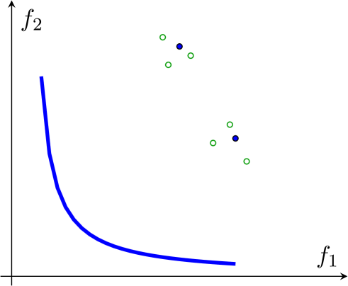
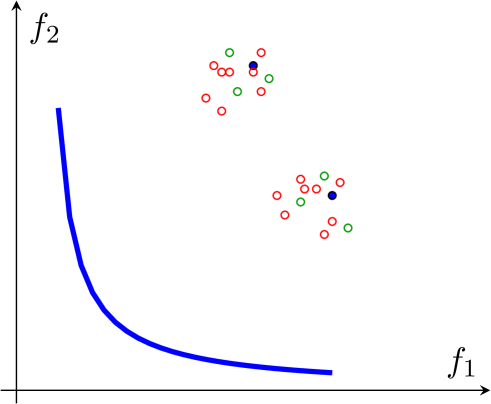
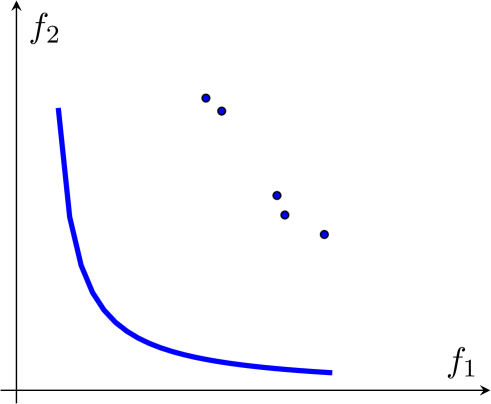
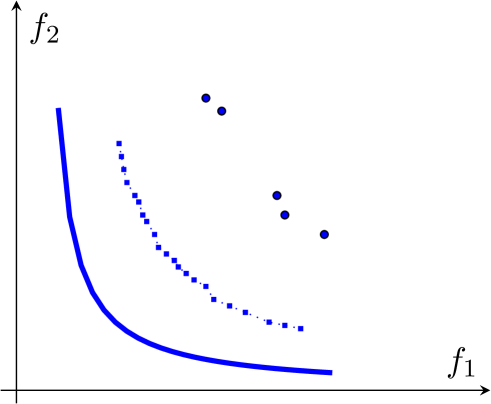
An illustration is provided in Figure 6. The blue curve represents the true Pareto front. The PF-SMG algorithm first randomly generates a list of starting feasible points (see blue points in Figure 6 (a)). For each point in the current list, a certain number of perturbed points (see green circles in Figure 6 (a)) are added to the list, after which multiple runs of the SMG algorithm are applied to each point in the current list. These newly generated points are marked by red circles in Figure 6 (b). At the end of the current iteration, a new list for the next iteration is obtained by removing all the dominated points. As the algorithm proceeds, the front will move towards the true Pareto front.
The complexity rates to determine a point in the Pareto front using stochastic multi-gradient are reported in (Liu & Vicente, 2021). However, in multiobjective optimization, as far as we know, there are no convergence or complexity results to determine the whole Pareto front (under reasonable assumptions that do not reduce to evaluating the objective functions in a set that is dense in the decision space).
Appendix C Metrics for Pareto front comparison
Let denote the set of algorithms/solvers and denote the set of test problems. The Purity metric measures the accuracy of an approximated Pareto front. Let us denote as an approximated Pareto front of problem computed by algorithm . We approximate the “true” Pareto front for problem by all the nondominated points in . Then, the Purity of a Pareto front computed by algorithm for problem is the ratio , which calculates the percentage of “true” nondominated solutions among all the nondominated points generated by algorithm . A higher ratio value corresponds to a more accurate Pareto front.
The Spread metric is designed to measure the extent of the point spread in a computed Pareto front, which requires the computation of extreme points in the objective function space . Among the objective functions, we select a pair of nondominated points in with the highest pairwise distance (measured using ) as the pair of extreme points. More specifically, for a particular algorithm , let denote the pair of nondominated points where and . Then, the pair of extreme points is with .
The first Spread formula calculates the maximum size of the holes for a Pareto front. Assume algorithm generates an approximated Pareto front with points, indexed by , to which the extreme points , indexed by and are added. Denote the maximum size of the holes by . We have
where , and we assume each of the objective function values is sorted in an increasing order.
The second formula was proposed by (Deb et al., 2002) for the case (and further extended to the case in (Custódio et al., 2011)) and indicates how well the points are distributed in a Pareto front. Denote the point spread by . It is computed by the following formula:
where is the average of over . Note that the lower and are, the more well distributed the Pareto front is.
Hypervolume (Zitzler & Thiele, 1999) is another classical performance indicator taking into account both the quality of the individual Pareto points and also their overall objective space coverage. It essentially calculates the area/volume dominated by the provided set of nondominated solutions with respect to a reference point. Figure 7 demonstrates a bi-objective case where the area dominated by a set of points with respect to the reference point is shown in grey. In our experiments, we calculate hypervolume using the Pymoo package (see https://pymoo.org/misc/indicators.html).
Appendix D Datasets generation and pre-processing
The synthetic data is formed by sets of 2,000 binary classification data instances randomly generated from the same distributions setting specified in Zafar et al. (2017b, Section 4), specifically using an uniform distribution for generating binary labels , two different Gaussian distributions for generating 2-dimensional nonsensitive features , and a Bernoulli distribution for generating the binary sensitive attribute .
The data pre-processing details for the Adult Income dataset are given below.
-
1.
First, we combine all instances in adult.data and adult.test and remove those that values are missing for some attributes.
-
2.
We consider the list of features: Age, Workclass, Education, Education number, Martial Status, Occupation, Relationship, Race, Sex, Capital gain, Capital loss, Hours per week, and Country. In the same way as the authors (Zafar et al., 2017a) did for attribute Country, we reduced its dimension by merging all non-United-Stated countries into one group. Similarly for feature Education, where “Preschool”, “1st-4th”, “5th-6th”, and “7th-8th” are merged into one group, and “9th”, “10th”, “11th”, and “12th” into another.
-
3.
Last, we did one-hot encoding for all the categorical attributes, and we normalized attributes of continuous value.
| Gender | Total | ||
|---|---|---|---|
| Males | |||
| Females | |||
| Total |
| Race | Total | ||
|---|---|---|---|
| Asian | |||
| American-Indian | |||
| White | |||
| Black | |||
| Other | |||
| Total |
| race | reoffend | Not reoffend | Total |
|---|---|---|---|
| White | |||
| Black | |||
| Total |
In terms of gender, the dataset contains males ( high income) and females ( high income). Similarly, the demographic compositions in terms of race are Asian (), American-Indian (), White (), Black (), and Other (), where the numbers in brackets are the percentages of high-income instances.
Appendix E More numerical results
E.1 Disparate impact w.r.t. binary sensitive attribute
E.2 Disparate impact w.r.t. multi-valued sensitive attribute
E.3 Streaming data