Accurate Summary-based Cardinality Estimation Through the Lens of Cardinality Estimation Graphs
Abstract.
We study two classes of summary-based cardinality estimators that use statistics about input relations and small-size joins in the context of graph database management systems: (i) optimistic estimators that make uniformity and conditional independence assumptions; and (ii) the recent pessimistic estimators that use information theoretic linear programs. We begin by addressing the problem of how to make accurate estimates for optimistic estimators. We model these estimators as picking bottom-to-top paths in a cardinality estimation graph (CEG), which contains sub-queries as nodes and weighted edges between sub-queries that represent average degrees. We outline a space of heuristics to make an optimistic estimate in this framework and show that effective heuristics depend on the structure of the input queries. We observe that on acyclic queries and queries with small-size cycles, using the maximum-weight path is an effective technique to address the well known underestimation problem for optimistic estimators. We show that on a large suite of datasets and workloads, the accuracy of such estimates is up to three orders of magnitude more accurate in mean q-error than some prior heuristics that have been proposed in prior work. In contrast, we show that on queries with larger cycles these estimators tend to overestimate, which can partially be addressed by using minimum weight paths and more effectively by using an alternative CEG. We then show that CEGs can also model the recent pessimistic estimators. This surprising result allows us to connect two disparate lines of work on optimistic and pessimistic estimators, adopt an optimization from pessimistic estimators to optimistic ones, and provide insights into the pessimistic estimators, such as showing that there are alternative combinatorial solutions to the linear programs that define them.
1. Introduction
The problem of estimating the output size of a natural multi-join query (henceforth join query for short), is a fundamental problem that is solved in the query optimizers of database management systems when generating efficient query plans. This problem arises both in systems that manage relational data as well those that manage graph-structured data where systems need to estimate the cardinalities of subgraphs in their input graphs. It is well known that both problems are equivalent, since subgraph queries can equivalently be written as join queries over binary relations that store the edges of a graph.
We focus on the prevalent technique used by existing systems of using statistics about the base relations or outputs of small-size joins to estimate cardinalities of joins. These techniques use these statistics in algebraic formulas that make independence and uniformity assumptions to generate estimates for queries (Aboulnaga et al., 2001; Maduko et al., 2008; Mhedhbi and Salihoglu, 2019; Neumann and Moerkotte, 2011). We will refer to these as summary-based optimistic estimators (optimistic estimators for short), to emphasize that these estimators can make both under and overestimations. This contrasts with the recent pessimistic estimators that are based on worst-case optimal join size bounds (Abo Khamis et al., 2016; Atserias et al., 2013; Cai et al., 2019; Gottlob et al., 2012; Joglekar and Ré, 2018) and avoid underestimation, albeit using very loose, so inaccurate, estimates (Park et al., 2020). In this work, we study how to make accurate estimations using optimistic estimators using a new framework that we call cardinality estimation graphs (CEGs) to represent them. We observe and address several shortcomings of these estimators under the CEG framework. We show that this framework is useful in two additional ways: (i) CEGs can also represent the pessimistic estimators, establishing that these two classes of estimators are in fact surprisingly connected; and (ii) CEGs are useful mathematical tools to prove several theoretical properties of pessimistic estimators.
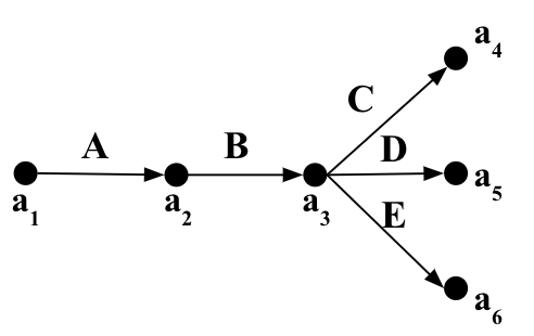
We begin by showing that the algebraic formulas of prior optimistic estimators can be modeled as picking a bottom-to-top path in a weighted CEG, which we call , for Optimistic. In this CEG nodes are intermediate sub-queries and edges weights are average degree statistics that extend sub-queries to larger queries. For example, consider the subgraph query in Figure 1 and the input dataset in Figure 2, whose is shown in Figure 3. We observe that in estimators that can be represented with CEGs, there is often more than one way to generate an estimate for a query, corresponding to different bottom-to-up paths and that this decision does not have a clear answer in the case of . For example, consider the subgraph query in Figure 1. Given that we have the accurate cardinalities of all subqueries of size 2 available, there are 252 formulas (or bottom-to-up paths in the CEG of optimistic estimators) to estimate the cardinality of the query. Examples of these formulas are:
In previous work (Aboulnaga et al., 2001; Maduko et al., 2008; Mhedhbi and Salihoglu, 2019), the choice of which of these estimates to use has either been unspecified or decided by a heuristic without acknowledging possible other choices or empirically justifying these choices. As our first main contribution, we systematically describe a space of heuristics for making an estimate for optimistic estimators and show empirically that the better performing heuristics depend on the structure of the query. We show that on acyclic queries and queries with small-size cycles, whose statistics are available, using the maximum-weight path through the CEG is an effective way to make accurate estimations. We observe that as in the relational setting, estimators that use independence assumptions tend to underestimate the true cardinalities on these queries, and the use of maximum-weight path in the CEG can offset these underestimations. In contrast we observe that on queries that contain larger cycles, the optimistic estimators estimate modified versions of these queries that break these cycles into paths, which leads to overestimations. We show that on such queries, using the minimum weight paths leads to generally more accurate estimations than other heuristics. However, we also observe that these estimates can still be highly inaccurate, and address this shortcoming by defining a new CEG for these queries, which we call , for Optimistic Cycle closing Rate, that use as edge weights statistics that estimate the probabilities that two edges that are connected through a path can close into a cycle. We further show that in general considering only the “long-hop” paths, i.e., with more number of edges, that make more independence assumption but by conditioning on larger sub-queries performs better than paths with fewer edges and comparably to considering every path.
As our second main contribution, we show that CEGs are expressive enough to model also the recent linear program-based pessimistic estimators. Specifically, we show that we can take and replace its edge weights (which are average degrees) with maximum degrees of base relations and small-size joins, and construct a new CEG, which we call , for MOLP bound from reference (Joglekar and Ré, 2018). We show that each path in is guaranteed to be an overestimate for the cardinality of the query, therefore picking the minimum weight path on this CEG would be the most accurate estimate. We show that this path is indeed equivalent to the MOLP pessimistic estimator from reference (Joglekar and Ré, 2018). The ability to model pessimistic estimators as CEGs allows us to make several contributions. First, we connect two seemingly disparate classes of estimators: both subgraph summary-based optimistic estimators and the recent LP-based pessimistic ones can be modeled as different instances of estimators that pick paths through CEGs. Second, this result sheds light into the nature of the arguably opaque LPs that define pessimistic estimators. Specifically we show that in addition to their numeric representations, the pessimistic estimators have a combinatorial representation. Third, we show that a bound sketch optimization from the recent pessimistic estimator from references (Cai et al., 2019) can be directly applied to any estimator using a CEG, specifically to the optimistic estimators, and empirically demonstrate its benefits in some settings.
CEGs further turn out to be very useful mathematical tools to prove certain properties of the pessimistic estimators, which may be of independent interest to readers who are interested in the theory of pessimistic estimators. Specifically using CEGs in our proofs, we show that MOLP can be simplified because some of its constraints are unnecessary, provide several alternative combinatorial proofs to some known properties of MOLP, such as the theorem that MOLP is tighter than another bound called DBPLP (Joglekar and Ré, 2018), and that MOLP is at least as tight as the pessimistic estimator proposed by Cai et al (Cai et al., 2019) and are identical on acyclic queries over binary relations.
The remainder of this paper is structured as follows. Section 2 provides our query and database notation. Section 3 gives an overvi-ew of generic estimators that can be seen as picking paths from a CEG. Section 4 reviews optimistic estimators that can be modeled with and outlines the space of possible heuristics for making estimates using . We also discuss the shortcoming of when estimating queries with large cycles and present to address this shortcoming. Section 5 reviews the pessimistic estimators, the of the MOLP estimator and the bound sketch refinement to pessimistic estimators. Using , we prove several properties of MOLP and connect some of these pessimistic estimators. Section 6 presents extensive experiments evaluating our space of optimistic estimators both on , and and the benefits of bound sketch optimization. We compare the optimistic estimators against other summary-based and sampling-based techniques and evaluate the effects of our estimators on plan quality on an actual system. We also confirm as in reference (Park et al., 2020) that the pessimistic estimators in our settings are also not competitive and lead to highly inaccurate estimates. Finally, Sections 7 and 8 cover related work and conclude, respectively.
2. Query and Database Notation
We consider conjunctive queries of the form
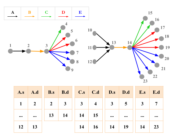
where is a relation with attributes and . Most of the examples used in this paper involve edge-labeled subgraph queries, in which case each is a binary relation containing a subset of the edges in a graph as source/destination pairs. Figure 2 presents an example showing a graph with edge labels , , , , and , shown in black, orange, green, red, and blue. This graph can be represented using five binary relations, one for each of the edge labels. These relations are also shown in Figure 2.
We will often represent queries over such relations using a graph notation. For example, consider the relations and from Figure 2. We will represent the query as . Similarly, the query will be represented as .
3. CEG Overview
Next, we offer some intution for cardinality estimation graphs (CEGs). In Sections 4 and 5 we will define specific CEGs corresponding to different classes of optimistic and pessimistic estimators. However, all of these share a common structure for representing cardinality estimations. Specifically, a CEG for a query will consist of:
-
Vertices labeled with subqueries of , where subqueries are defined by subsets of ’s relations or attributes.
-
Edges from smaller subqueries to larger subqueries, labeled with extension rates which represent the cardinality of the larger subquery relative to that of the smaller subquery.
Each bottom-to-top path (from to ) in a CEG represents a different way of generating a cardinality estimate for . An estimator using a CEG picks one of these paths as an estimate. The estimate of a path is the product of the extension rates along the edges of the path. Equivalently one can put the logarithms of the extension rates as edge weights and sum the logarithms (and exponentiate the base of the logarithm) to compute the estimate.
Figure 4 illustrates a 111Specifically, it is a , defined in Section 4. for the query shown in Figure 1 over the relations shown in Figure 2, assuming that statistics are available for any size-2 subqueries of . For example, the leftmost path starts with , then extends to , then to the subquery of 4-fork involving , , , and , and finally extends the 4-fork subquery to . The first extension rate from to is simply the known cardinality of , which is 4, and the second extension rate makes the uniformity assumption of . The final estimate of this path is .
In the rest of this paper, we will show how some of the optimistic and pessimistic estimators from literature can be modeled as instances of this generic estimator using different CEGs. We will show that while it is clear that the minimum-weight path should be the estimate chosen in the CEG of pessimistic estimators, it is not clear which path should be chosen from the CEG of optimistic estimators. We will also discuss a shortcoming of the CEG for optimistic estimators and address it by defining a new CEG.
4. Optimistic Estimators
The estimators that we refer to as optimistic in this paper use known statistics about the input database in formulas that make uniformity and independence or conditional independence assumptions. The cardinality estimators of several systems fall under this category. We focus on three estimators: Markov tables (Aboulnaga et al., 2001) from XML databases, graph summaries (Maduko et al., 2008) from RDF databases, and the graph catalogue estimator of the Graphflow system (Mhedhbi and Salihoglu, 2019) for managing property graphs. These estimators are extensions of each other and use the statistics of the cardinalities of small-size joins. We give an overview of these estimators and then describe their CEGs, which we will refer to as , and then first describe a space of possible optimistic estimates that an optimistic estimator can make. We then discuss a shortcoming of the when queries contain large cycles whose statistics are missing and describe a modification to to make more accurate estimations.
4.1. Overview
We begin by giving an overview of the Markov tables estimator (Aboulnaga et al., 2001), which was used to estimate the cardinalities of paths in XML documents. A Markov table of length stores the cardinality of each path in an XML document’s element tree up to length and uses these to make predications for the cardinalities of longer paths. Table 1 shows a subset of the entries in an example Markov table for for our running example dataset shown in Figure 2. The formula to estimate a 3-path using a Markov table with is to multiply the cardinality of the leftmost 2-path with the consecutive 2-path divided by the cardinality of the common edge. For example, consider the query against the dataset in Figure 2. The formula for would be: . Observe that this formula is inspired by the Bayesian probability rule that but makes a conditional independence assumption between and , in which case the Bayesian formula would simplify to . For the formula uses the true cardinality . For the formula makes a uniformity assumption that the number of edges that each edge extends to is equal for each edge and is . Equivalently, this can be seen as an “average degree” assumption that on average the -degree of nodes in the paths is . The result of this formula is , which underestimates the true cardinality of 7. The graph summaries (Maduko et al., 2008) for RDF databases and the graph catalogue estimator (Mhedhbi and Salihoglu, 2019) for property graphs have extended the contents of what is stored in Markov tables, respectively, to other acyclic joins, such as stars, and small cycles, such as triangles, but use the same uniformity and conditional independence assumptions.
| Path | |Path| |
|---|---|
| 2 | |
| 4 | |
| 3 | |
| … | … |
4.2. Space of Possible Optimistic Estimators
We next represent such estimators using a CEG that we call . This will help us describe the space of possible estimations that can be made with these estimators. We assume that the given query is connected. consists of the following:
-
Vertices: For each connected subset of relations of , we have a vertex in with label . This represents the sub-query .
-
Edges: Consider two vertices with labels and s.t., . Let , for difference be , and let , for extension be a join query in the Markov table, and let , for intersection, be . If and exist in the Markov table, then there is an edge with weight from to in .
When making estimates, we will apply two basic rules from prior work that limit the paths considered in . First is that if the Markov table contains size- joins, the formulas use size joins in the numerators in the formula. For example, if , we do not try to estimate the cardinality of a sub-query by a formula because we store the true cardinality of in the Markov table. Second, for cyclic graph queries, which was covered in reference (Mhedhbi and Salihoglu, 2019), an additional early cycle closing rule is used in the reference when generating formulas. In CEG formulation this translates to the rule that if can extend to multiple s and some of them contain additional cycles that are not in , then only such outgoing edges of to such are considered in finding paths.
Even when the previous rules are applied to limit the number of paths considered in a CEG, in general there may be multiple paths that lead to different estimates. Consider the shown in Figure 4 which uses a Markov table of size 2. There are 36 paths leading to 7 different estimates. Two examples are:
Similarly, consider the fork query in Figure 1 and a Markov table with up to 3-size joins. The of is shown in Figure 3, which contains multiple paths leading to 2 different estimates:
Both formulas start by using . Then, the first “short-hop” formula makes one fewer conditional independence assumption than the “long-hop” formula, which is an advantage. In contrast, the first estimate also makes a uniformity assumption that conditions on a smaller-size join. We can expect this assumption to be less accurate than the two assumptions made in the long-hop estimate, which condition on 2-size joins. In general, these two formulas can lead to different estimates.
For many queries, there can be many more than 2 different estimates. Therefore, any optimistic estimator implementation needs to make choices about which formulas to use, which corresponds to picking paths in . Prior optimistic estimators have either left these choices unspecified or described procedures that implicitly pick a specific path yet without acknowledging possible other choices or empirically justifying their choice. Instead, we systematically identify a space of choices that an optimistic estimator can make along two parameters that also capture the choices made in prior work:
-
Path length: The estimator can identify a set of paths to consider based on the path lengths, i.e., number of edges or hops, in , which can be: (i) maximum-hop (max-hop); (ii) minimum-hop (min-hop); or (iii) any number of hops (all-hops).
-
Estimate aggregator: Among the set of paths that are considered, each path gives an estimate. The estimator then has to aggregate these estimates to derive a final estimate, for which we identify three heuristics: (i) the largest estimated cardinality path (max-aggr); (ii) the lowest estimated cardinality path (min-aggr); or (iii) the average of the estimates among all paths (avg-aggr).
Any combination of these two choices can be used to design an optimistic estimator. The original Markov tables (Aboulnaga et al., 2001) chose the max-hop heuristic. In this work, each query was a path, so when the first heuristic is fixed, any path in leads to the same estimate. Therefore an aggregator is not needed. Graph summaries (Maduko et al., 2008) uses the min-hop heuristic and leaves the aggregator unspecified. Finally, graph catalogue (Mhedhbi and Salihoglu, 2019) picks the min-hop and min-aggr aggregator. We will do a systematic empirical analysis of this space of estimators in Section 6. In fact, we will show that which heuristic to use depends on the structure of the query. For example, on acyclic queries unlike the choice in reference (Mhedhbi and Salihoglu, 2019), systems can combat the well known underestimation problem of optimistic estimators by picking the ‘pessimistic’ paths, so using max-aggr heuristic. Similarly, we find that using the max-hop heuristic leads generally to highly accurate estimates.
4.3. : Handling Large Cyclic Patterns
Recall that a Markov table stores the cardinalities of patterns up to some size . Given a Markov table with , optimistic estimators can produce estimates for any acyclic query with size larger than . But what about large cyclic queries, i.e., cyclic queries with size larger than ?
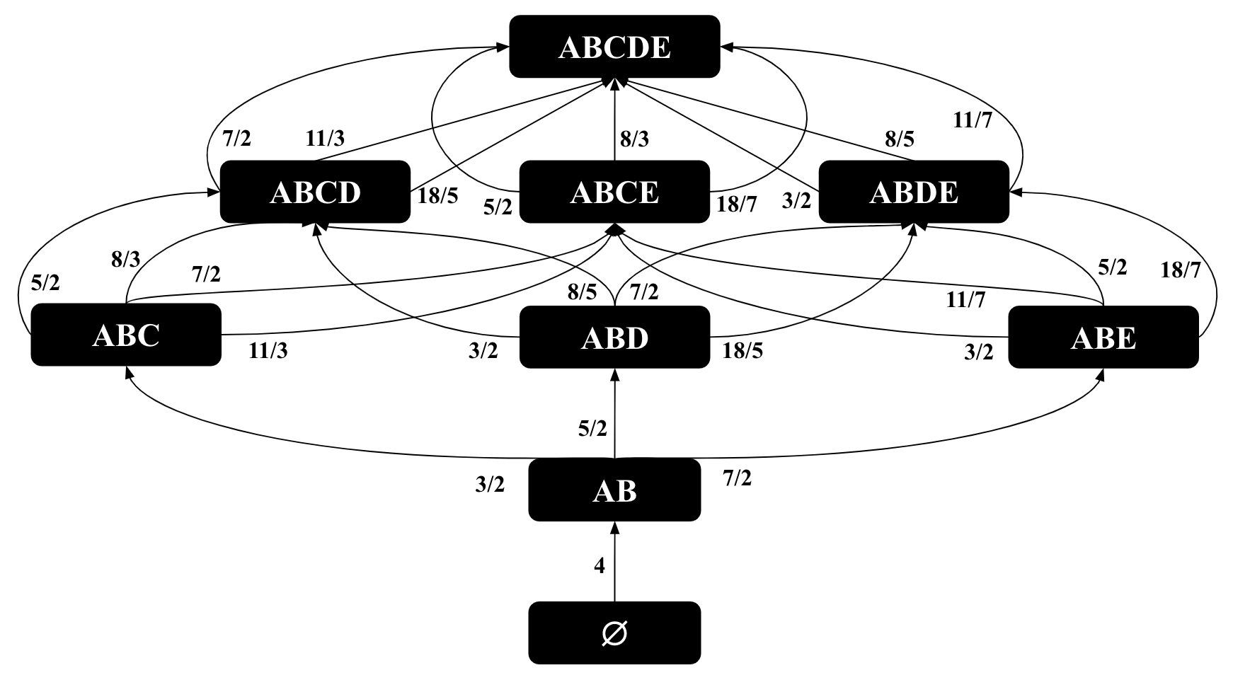
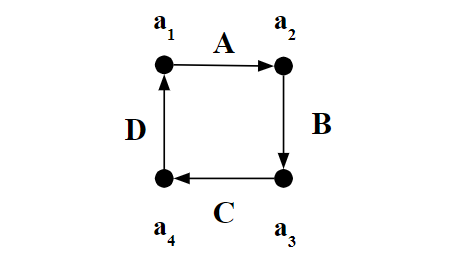
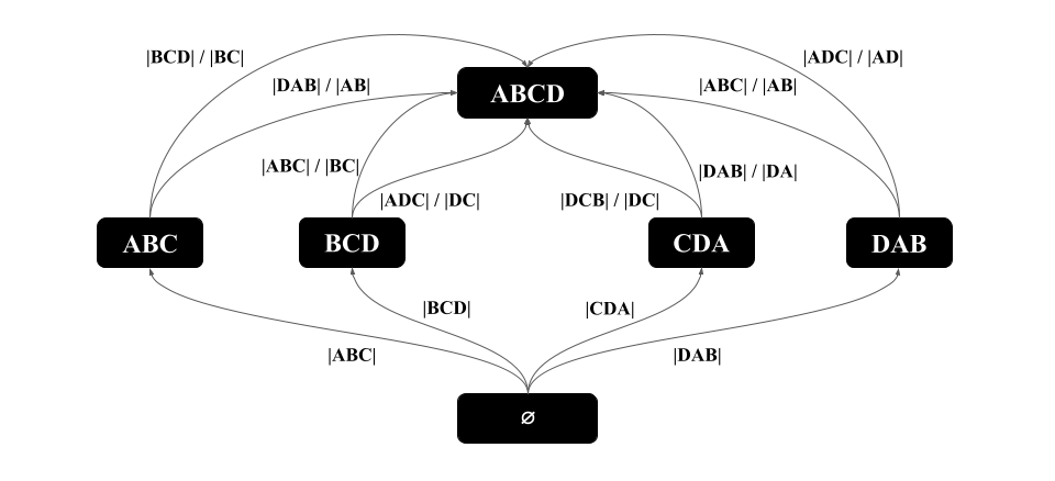
Faced with a large cyclic query , the optimistic estimators we have described do not actually produce estimates for . Instead, they produce an estimate for a similar acyclic that includes all of ’s edges but is not closed. To illustrate this, consider estimating a 4-cycle query in Figure 5 using a Markov table with =. Recall that the estimates of prior optimistic estimators are captured by paths in the for 4-cycle query, shown in Figure 6(a). Consider as an example, the left most path, which corresponds to the formula: . Note that this formula is in fact estimating a 4-path rather than the 4-cycle shown in Figure 5. This is true for each path in .
More generally, when queries contain cycles of length , breaks cycles in queries into paths. Although optimistic estimators generally tend to underestimate acyclic queries due to the independence assumptions they make, the situation is different for cyclic queries. Since there are often significantly more paths than cycles, estimates over can lead to highly inaccurate overestimates. We note that this problem does not exist if a query contains a cycle of length that contains smaller cycles in them, such as a clique of size , because the early cycle closing rule from Section 4.2 will avoid formulas that estimate as a sub-query (i.e., no sub-path will exist in CEG).
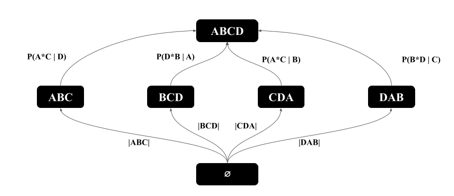
We next describe an alternative modified CEG to address this problem. Consider a query with a -cycle where . Note that in order to not break cycles into paths, we need CEG edges whose weights capture the cycle closing effect when extending a sub-query that contains edges of to a sub-query that contains . We capture this in a new CEG called , for Optimistic Cycle closing Rate, which modifies as follows. We keep the same vertices as in and the same set of edges, except when we detect two vertices and with the above property. Then, instead of using the weights from the original between and , we use pre-computed cycle closing probabilities. Suppose the last edge that closes the cycle is and it is between the query edges and . In the Markov table, we store the probabilities of two connected and edges to be connected by an additional edge to close a cycle. We denote this statistic as . We can compute by computing all paths that start from and end with of varying lengths and then counting the number of edges that close such paths to cycles. On many datasets there may be a prohibitively many such paths, so we can sample of such paths. Suppose these paths lead to many cycles, then we can take the probability as . In our implementation we perform sampling through random walks that start from and end at but other sampling strategies can also be employed. Figure 6(b) provides the for the 4-cycle query in Figure 5. We note that the Markov table for requires computing additional statistics that does not require. The number of entries is at most where is the number of edge labels in the dataset. For many datasets, e.g., all of the ones we used in our evaluations, is small and in the order of 10s or 100s, so even in the worst case these entries can be stored in several MBs. In contrast, storing large cycles with edges could potentially require more entries.
5. Pessimistic Estimators
Join cardinality estimation is directly related to the following fundamental question: Given a query and set of statistics over the relations , such as their cardinalities or degree information about values in different columns, what is the worst-case output size of ? Starting from the seminal result by Atserias, Grohe, and Marx in 2008 (Atserias et al., 2013), several upper bounds have been provided to this question under different known statistics. For example the initial upper bound from reference (Atserias et al., 2013), now called the AGM bound, used only the cardinalities of each relation, while later bounds, DBPLP (Joglekar and Ré, 2018), MOLP (Joglekar and Ré, 2018), and CLLP (Abo Khamis et al., 2016) used maximum degrees of the values in the columns and improved the AGM bound. Since these bounds are upper bounds on the query size, they can be used as pessimistic estimators. This was done recently by Cai et al. (Cai et al., 2019) in an actual estimator implementation. We refer to this as the CBS estimator, after the names of the authors.
In this section, we show a surprising connection between the optimistic estimators from Section 4 and the recent pessimistic estimators (Joglekar and Ré, 2018; Cai et al., 2019). Specifically, in Section 5.1, we show that similar to optimistic estimators, MOLP (and CBS) can also be modeled as an estimator using a CEG. CEGs further turn out to be useful mathematical tools to prove properties of pessimistic estimators. We next show applications of CEGs is several of our proofs to obtain several theoretical results that provide insights into the pessimistic estimators. Section 5.2 reviews the CBS estimator. Using our CEG framework, we show that in fact the CBS estimator is equivalent to the MOLP bound on acyclic queries on which it was evaluated in reference (Cai et al., 2019). In Section 5.2, we also review the bound sketch refinement of the CBS estimator from reference (Cai et al., 2019), which we show can also be applied to any estimator using a CEG, specifically the optimistic ones we cover in this paper. Finally, Appendix D reviews the DBPLP bound and provides an alternative proof that MOLP is tighter than DBPLP that also uses CEGs in the proof.
5.1. MOLP
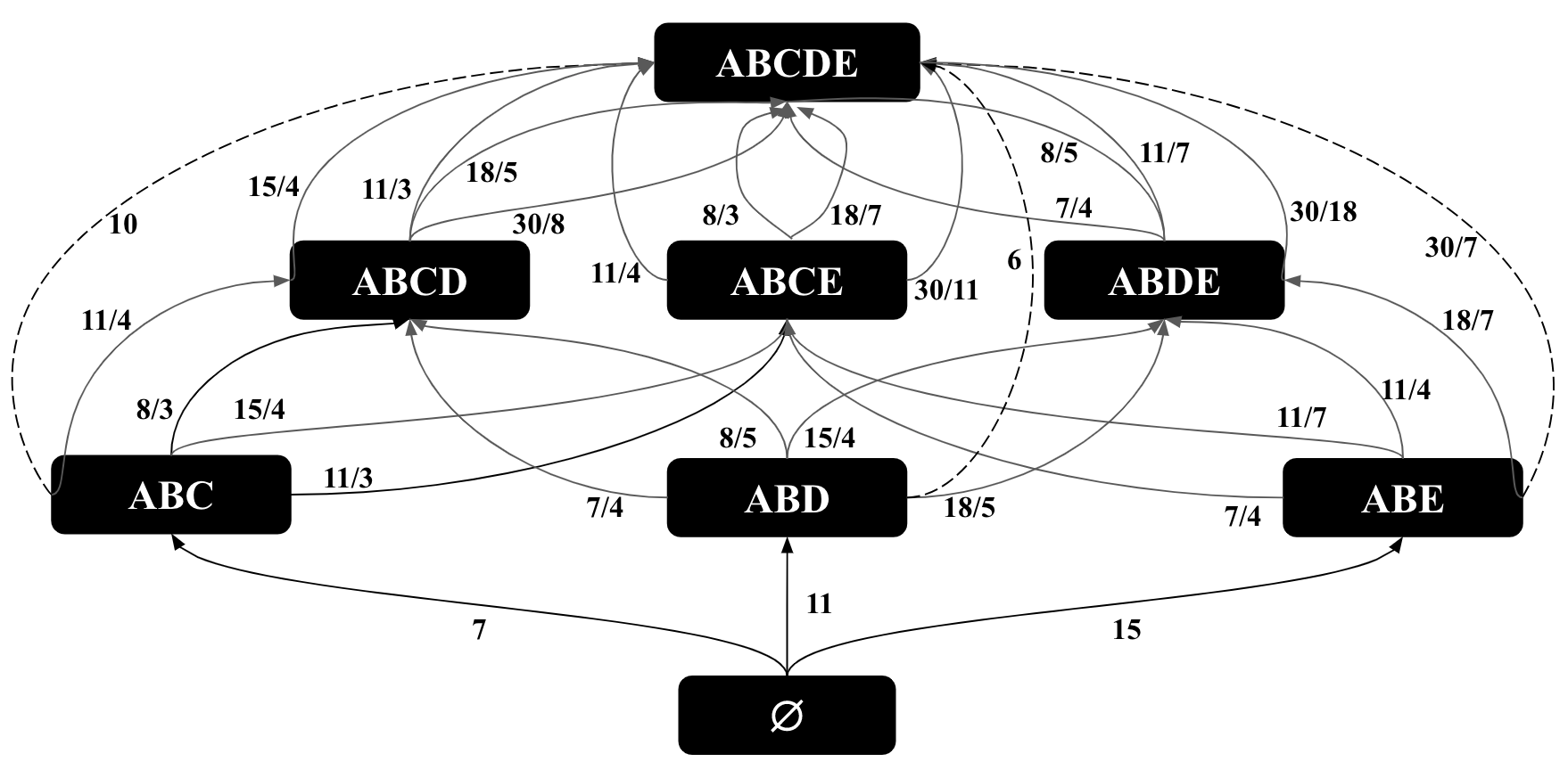
MOLP was defined in reference (Joglekar and Ré, 2018) as a tighter bound than the AGM bound that uses additional degree statistics about input relations that AGM bound does not use. We first review the formal notion of a degree. Let be a subset of the attributes of some relation , and let be a possible value of . The degree of in is the number of times occurs in , i.e. . For example, in Figure 2, because the outgoing -degree of vertex 3 is 3. Similarly is 1 because the incoming -degree of vertex 2 is 1. We also define to be the maximum degree in of any value over , i.e., . So, because vertex 13 has 3 incoming edges, which is the maximum A-in-degree in the dataset. The notion of degree can be generalized to , which refers to the “degree of a value over attributes in ”, which counts the number of times occurs in . Similarly, we let . Suppose a system has stored statistics for each possible and . MOLP is:
The base of the logarithm can be any constant and we take it as 2. Let be the optimal value of MOLP. Reference (Joglekar and Ré, 2018) has shown that is an upper bound on the size of . For example, in our running example, the optimal value of these inequalities is 96, which is an overestimate of the true cardinality of 78. It is not easy to directly see the solution of the MOLP on our running example. However, we will next show that we can represent the MOLP bound as the cost of minimum-weight path in a CEG that we call .
MOLP CEG (): Let be the projection of onto attributes , so . Each variable in MOLP represents the maximum size of , i.e., the tuples in the projection of that contribute to the final output. We next interpret the two sets of inequalities in MOLP:
-
Extension Inequalities : These inequalities intuitively indicate the following: each tuple can extend to at most tuples. For example, in our running example, let , and . So both and are subsets of . The inequality indicates that each tuple, so an tuple, can extend to at most tuples. This is true, because is the maximum degree of any value in (in graph terms the maximum degree of any vertex with an outgoing edge).
-
Projection Inequalities : These indicate that the number of tuples in is at most the number of , if is a larger subquery.
With these interpretations we can now construct .
-
Vertices: For each there is a vertex. This represents the subquery .
-
Extension Edges: Add an edge with weight between any and , for which there is inequality. Note that there can be multiple edges between and corresponding to inequalities from different relations.
-
Projection Edges: , add an edge with weight 0 from to . These edges correspond to projection inequalities and intuitively indicate that, in the worst-case instances, is always as large as .
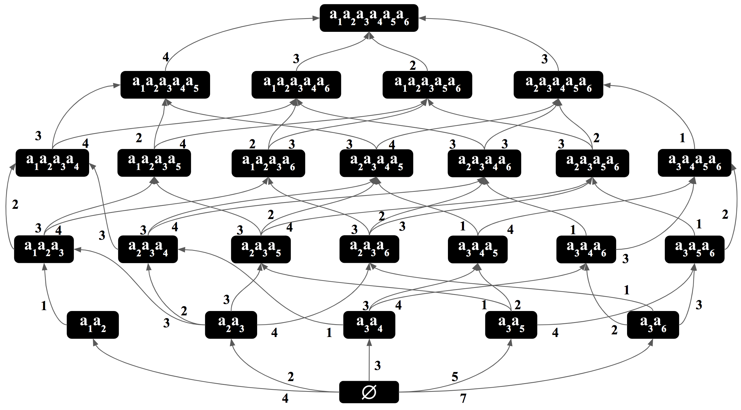
Figure 7 shows the of our running example. For simplicity, we use actual degrees instead of their logarithms as edge weights and omit the projection edges in the figure. Below we use instead of , to represent the bottom-to-top paths in because .
Theorem 5.1.
Let be a query whose degree statistics for each and is known. The optimal solution to the MOLP of is equal to the weight of the minimum-weight path in CEGM.
Proof.
Our proof consists of two steps. First we show that any feasible solution to MOLP has a value at most the weight of any path. Then we show that a particular feasible solution, which we call , is exactly the weight of the minimum-weight path. Let be a feasible solution to the . We refer to the value of , so the value takes in , simply as . Let be any path in . Let be the weight of . Suppose w.l.o.g. that … and for the purpose of contradiction that . If this is the case, we can inductively (from down to ) show that . The base case for holds by our assumption. Suppose by induction hypothesis. Then consider the inequality in that corresponds to the edge . There are two possible cases for this inequality:
Case 1: is a projection edge, so and we have an inequality of , so , so .
Case 2: is an extension edge, so we have an inequality of , so , so , completing the inductive proof. However, this implies that , which contradicts the first inequality of MOLP, completing the proof that any feasible solution to the MOLP is at most the weight of any path in .
Next, let be an assignment of variables that sets each to the weight of the minimum-weight path in . Let be the value of in . We show that is a feasible solution to . First, note that in is assigned a value of 0, so the first inequality of MOLP holds. Second, consider any extension inequality , so contains an edge from to with weight . By definition of minimum-weight paths, . Therefore, in all of the extension inequalities hold. Finally, consider a projection inequality , where , so contains an edge from vertex to vertex with weight 0. By definition of minimum-weight paths, , so all of these inequalities also hold. Therefore, is indeed a feasible solution to . Since any solution to MOLP has a value smaller than the weight of any path in , we can conclude that in , which is the minimum-weight path, is equal to . ∎
With this connection, readers can verify that the MOLP bound in our running example is 96 by inspecting the paths in Figure 7. In this CEG, the minimum-weight path has a length of 96 (specifically ), corresponding to the leftmost path in Figure 7. We make three observations.
Observation 1: Similar to the CEGs for optimistic estimators, each path in corresponds to a sequence of extensions from to and is an estimate of the cardinality of . For example, the rightmost path in Figure 7 indicates that there are ’s (so edges), each of which extends to at most 3 ’s (so edges), and so forth. This path yields 7x3x2x1x3=126 many possible outputs. Since we are using maximum degrees on the edge weights, each path is by construction an upper bound on . So any path in is a pessimistic estimator. This is an alternative simple proof to the following proposition:
Proposition 5.0 (Prop. 2 (Joglekar and Ré, 2018)).
Let be a join query and be the output size of , then .222This is a slight variant of Prop. 2 from reference (Joglekar and Ré, 2018), which state that another bound, called the MO bound, which adds a preprocessing step to MOLP, is an upper bound of .
Proof.
Since for any (, ) path in , and by Theorem 5.1, is equal to the weight of the minimum-weight (, ) path in , . ∎
Observation 2: Theorem 5.1 implies that MOLP can be solved using a combinatorial algorithm, e.g., Dijkstra’s algorithm, instead of a numeric LP solver.
Observation 3: Theorem 5.1 implies that we can simplify MOLP by removing the projection inequalities, which correspond to the edges with weight 0 in . To observe this, consider any path … and consider its first projection edge, say . In Appendix A, we show that we can remove and construct an alternative path with at most the same weight as but with one fewer projection edge, showing that MOLP linear program can be simplified by only using the extension inequalities.
5.1.1. Using Degree Statistics of Small-Size Joins
MOLP can directly integrate the degree statistics from results of small-size joins. For example, if a system knows the size of , then the MOLP can include the inequality that . Similarly, the extension inequalities can use the degree information from simply by taking the output of as an additional relation in the query with three attributes , , and . When comparing the accuracy of the MOLP bound with optimistic estimators, we will ensure that MOLP uses the degree information of the same small-size joins as optimistic estimators, ensuring that MOLP uses a strict superset of the statistics used by optimistic estimators.
5.2. CBS and Bound Sketch Optimization
We review the CBS estimator very briefly and refer the reader to reference (Cai et al., 2019) for details. CBS estimator has two subroutines Bound Formula Generator (BFG) and Feasible Coverage Generator (FCG) (Algorithms 1 and 2 in reference (Cai et al., 2019)) that, given a query and the degree statistics about , generate a set of bounding formulas. A coverage is a mapping (, of a subset of the relations in the query to attributes such that each appears in the mapping. A bounding formula is a multiplication of the known degree statistics that can be used as an upper bound on the size of a query. In Appendix B, we show using our CEG framework that in fact the MOLP bound is at least as tight as the CBS estimator on general acyclic queries and is exactly equal to the CBS estimator over acyclic queries over binary relations, which are the queries which reference (Cai et al., 2019) used. Therefore BFG and FCG can be seen as a method for solving the MOLP linear program on acyclic queries over binary relations, albeit in a brute force manner by enumerating all paths in . We do this by showing that each path in corresponds to a bounding formula and vice versa. These observations allow us to connect two worst-case upper bounds from literature using CEGs. Henceforth, we do not differentiate between MOLP and the CBS estimator. It is important to note that a similar connection between MOLP and CBS cannot be established for cyclic queries. This is because, although not explicitly acknowledged in reference (Cai et al., 2019), on cyclic queries, the covers that FCG generates may not be safe, i.e., the output of BFG may not be a pessimistic output. We provide a counter example in Appendix C. In contrast, MOLP generates a pessimistic estimate for arbitrary, so both acyclic or cyclic, queries.
5.2.1. Bound Sketch
We next review an optimization that was described in reference (Cai et al., 2019) to improve the MOLP bound. Given a partitioning budget , for each bottom-to-top path in CEGM, the optimization partitions the input relations into multiple pieces and derives many subqueries of . Then the estimate for is the sum of estimates of all subqueries. Intuitively, partitioning decreases the maximum degrees in subqueries to yield better estimates, specifically their sum is guaranteed to be more accurate than making a direct estimate for . We give an overview of the optimization here and refer the reader to reference (Cai et al., 2019) for details.
We divide the edges in into two. Recall that each edge in is constructed from an inequality of in MOLP. We call (i) an unbound edge if , i.e., the weight of is ; (ii) a bound edge if , i.e., the weight of is actually the degree of some value in a column of . Note that unbound edge extends exactly with attributes , i.e., and a bound edge with attributes , i.e., . Below, we refer to these attributes as “extension” attributes.
Step1: For each path in (so a bounding formula in the terminology used in reference (Cai et al., 2019)), let be the join attributes that are not extension attributes through a bounded edge. For each attribute in , allocate partitions. For example, consider the path in the of from Figure 7, where refers to . Then both and would be in . For path , only would be in in .
Step2: Partition each relation as follows. Let , for partition attributes, be and be . Then partition into pieces using hash functions, each hashing a tuple based on one of the attributes in into . For example, the relation in our example path would be partitioned into 4, , , , and .
Step3: Then divide into components , to , such that contains only the partitions of each relation that matches the indices. For example, in our example, is . This final partitioning is called the bound sketch of for path .
5.2.2. Implementing Bound Sketch in Opt. Estimators
Note that a bound sketch can be directly used to refine any estimator using a CEG, as it is a general technique to partition into subqueries based on each path in a CEG. The estimator can then sum the estimates for each subquery to generate an estimate for . Specifically, we can use a bound sketch to refine optimistic estimators and we will evaluate its benefits in Section 6.3. Intuitively, one advantage of using a bound sketch is that the tuples that hash to different buckets of the join attributes are guaranteed to not produce outputs and they never appear in the same subquery. This can make the uniformity assumptions in the optimistic estimators more accurate because two tuples that hashed to the same bucket of an attribute are more likely to join.
We implemented the bound sketch optimization for optimistic estimators as follows. Given a partitioning budget and a set of queries in a workload, we worked backwards from the queries to find the necessary subqueries, and for each subquery the necessary statistics that would be needed are stored in the Markov table. For example, for , one of the formulas that is needed is: , so we ensure that our Markov table has these necessary statistics.
6. Evaluation
We next present our experiments, which aim to answer five questions: (1) Which heuristic out of the space we identified in Section 4.2 leads to better accuracy for optimistic estimators, and why? We aim to answer this question for acyclic queries on and cyclic queries on and . (2) For cyclic queries, which of these two CEGs lead to more accurate results under their best performing heuristics? (3) How much does the bound-sketch optimization improve the optimistic estimators’ accuracy? (4) How do optimistic and pessimistic estimators, which are both summary-based estimators, compare against each other and other baseline summary-based estimators from the literature? (5) How does the best-performing optimistic estimator compare against Wander Join (Li et al., 2016; Park et al., 2020), the state-of-the-art sampling-based estimator? Finally, as in prior work, we use the RDF-3X system (Neumann and Weikum, 2008) to verify that our estimators’ more accurate estimations lead more performant query plans.
Throughout this section, except in our first experiments, where we set , we use a Markov table of size for optimistic estimators. We generated workload-specific Markov tables, which required less than 0.6MB memory for any workload-dataset combination for or . For , which requires computing the cycle closing rates, the size was slightly higher but at most 0.9MB. Our code, datasets, and queries are publicly available at https://github.com/cetechreport/CEExperiments and https://github.com/cetechreport/gcare.
6.1. Setup, Datasets and Workloads
For all of our experiments, we use a single machine with two Intel E5-2670 at 2.6GHz CPUs, each with 8 physical and 16 logical cores, and 512 GB of RAM. We represent our datasets as labeled graphs and queries as edge-labeled subgraph queries but our datasets and queries can equivalently be represented as relational tables, one for each edge label, and SQL queries. We focused on edge-labeled queries for simplicity. Estimating queries with vertex labels can be done in a straightforward manner both for optimistic and pessimistic estimators e.g., by extending Markov table entries to have vertex labels as was done in reference (Mhedhbi and Salihoglu, 2019). We used a total of 6 real-world datasets, shown in Table 2, and 5 workloads on these datasets. Our dataset and workload combinations are as follows.
| Dataset | Domain | |V| | |E| | |E. Labels| |
|---|---|---|---|---|
| IMDb | Movies | 27M | 65M | 127 |
| YAGO | Knowledge Graph | 13M | 16M | 91 |
| DBLP | Citations | 23M | 56M | 27 |
| WatDiv | Products | 1M | 11M | 86 |
| Hetionet | Social Networks | 45K | 2M | 24 |
| Epinions | Consumer Reviews | 76K | 509K | 50 |
IMDb and JOB: The IMDb relational database, together with a workload called JOB, has been used for cardinality estimation studies in prior work (Cai et al., 2019; Leis et al., 2018). We created property graph versions of the this database and workload as follows. IMDb contains three groups of tables: (i) entity tables representing entities, such as actors (e.g., name table), movies, and companies; (ii) relationship tables representing many-to-many relationships between the entities (e.g., the movie_companies table represents relationships between movies and companies); and (iii) type tables, which denormalize the entity or relationship tables to indicate the types of entities or relationships. We converted each row of an entity table to a vertex. We ignored vertex types because many queries in the JOB workload have no predicates on entity types. Let and be vertices representing, respectively, rows and from tables an . We added two sets of edges between and : (i) a foreign key edge from to if the primary key of row is a foreign key in row ; (ii) a relationship edge between to if a row in a relationship table connects row and .
We then transformed the JOB workload (Leis et al., 2018) into equivalent subgraph queries on our transformed graph. We removed non-join predicates in the queries since we are focusing on join cardinality estimations, and we encoded equality predicates on types directly on edge labels. This resulted in 7 join query templates, including four 4-edge queries, two 5-edge queries, and one 6-edge query. All of these queries are acyclic. There were also 2- and 3-edge queries, which we ignored because as their estimation is trivial with Markov tables of size 3. We generated 100 query instances from each template by choosing one edge label uniformly at random for each edge, while ensuring that the output of the query was non-empty. The final workload contained a total of 369 specific query instances.
YAGO and G-CARE-Acyclic and G-CARE Cyclic Workloads: G-CARE (Park et al., 2020) is a recent cardinality estimation benchmark for subgraph queries. From this benchmark we took the YAGO knowledge graph dataset and the acyclic and cyclic query workloads for that dataset. The acyclic workload contains 382 queries generated from query templates with 3-, 6-, 9-, and 12-edge star and path queries, as well as randomly generated trees. We will refer to this workload as G-CARE-Acyclic. The cyclic query workload contains 240 queries generated from templates with 6-, and 9-edge cycle, 6-edge clique, 6-edge flower, and 6- and 9-edge petal queries. We will refer to this workload as G-CARE-Cyclic. The only other large dataset from G-CARE that was available was LUBM, which contained only 6 queries, so we did not include it in our study.
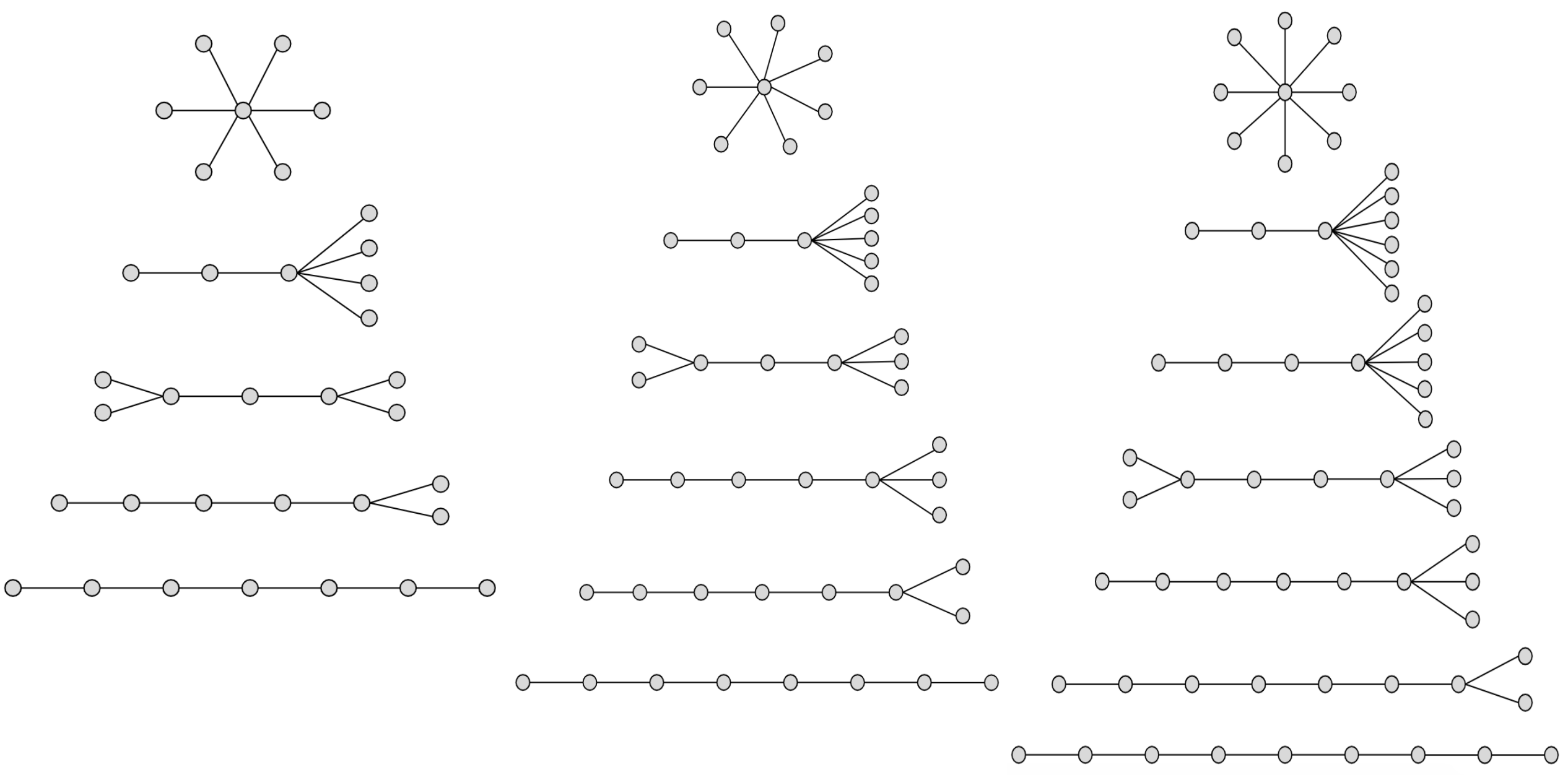
DBLP, WatDiv, Hetionet, and Epinions Datasets and Acyclic and Cyclic Workloads: We used four other datasets: (i) Hetionet: a biological network; (ii) DBLP: a real knowledge graph; (iii) WatDiv: a synthetic knowlege graph; and (iv) Epinions: a real-world social network graph. Epinions is a dataset that by default does not have any edge labels. We added a random set of 50 edge labels to Epinions. Our goal in using Epinions was to test whether our experimental observations also hold on a graph that is guranteed to not have any correlations between edge labels. For these datasets we created one acyclic and one cyclic query workload, which we refer to as Acyclic and Cyclic. The Acyclic workload contains queries generated from 6-, 7-, or 8-edge templates. We ensured that for each query size , we had patterns of every possible depth. Specifically for any , the minimum depth of any query is 2 (stars) and the maximum is (paths). For each depth in between, we picked a pattern. These patterns are shown in Figure 8. Then, we generated 20 non-empty instances of each template by putting one edge label uniformly at random on each edge, which yielded 360 queries in total. The Cyclic workload contains queries generated from templates used in reference (Mhedhbi and Salihoglu, 2019): 4-edge cycle, 5-edge diamond with a crossing edge, 6-cycle, complete graph , 6-edge query of two triangles with a common vertex, 8-edge query of a square with two triangles on adjacent sides, and a 7-edge query with a square and a triangle. We then randomly generated instances of these queries by randomly matching each edge of the query template one at a time in the datasets with a 1 hour time limit for each dataset. We generated 70 queries for DBLP, 212 queries for Hetionet, 129 queries for WatDiv, and 394 queries for Epinions.
6.2. Space of Optimistic Estimators
We begin by comparing the 9 optimistic estimators we described on the two optimistic CEGs we defined. In order to set up an experiment in which we could test all of the 9 possible optimistic estimators, we used a Markov table that contained up to 3-size joins (i.e., h=3). A Markov table with only 2-size joins can not test different estimators based on different path-length heuristics or any cyclic query. We aim to answer four specific questions: (1) Which of the 9 possible optimistic estimators we outlined in Section 4.2 leads to most accurate estimates on acyclic queries and cyclic queries that contain edges on ? (2) Which of the 9 estimators lead to most accurate estimates for cyclic queries with cycles of size on and ? (3) Which of these CEGs lead to most accurate estimations under their best performing estimators? (4) Given the accuracies of best performing estimators, how much room for improvement is there for designing more accurate techniques, e.g., heuristics, for making estimates on and ?
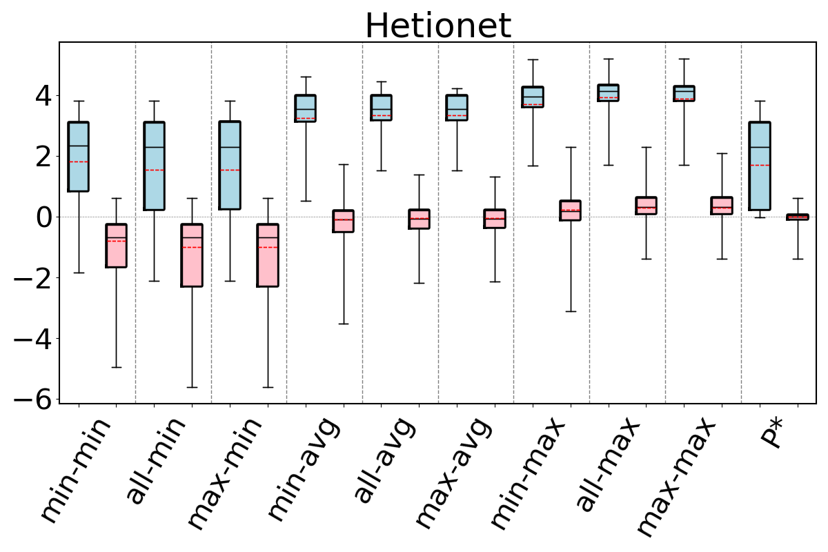
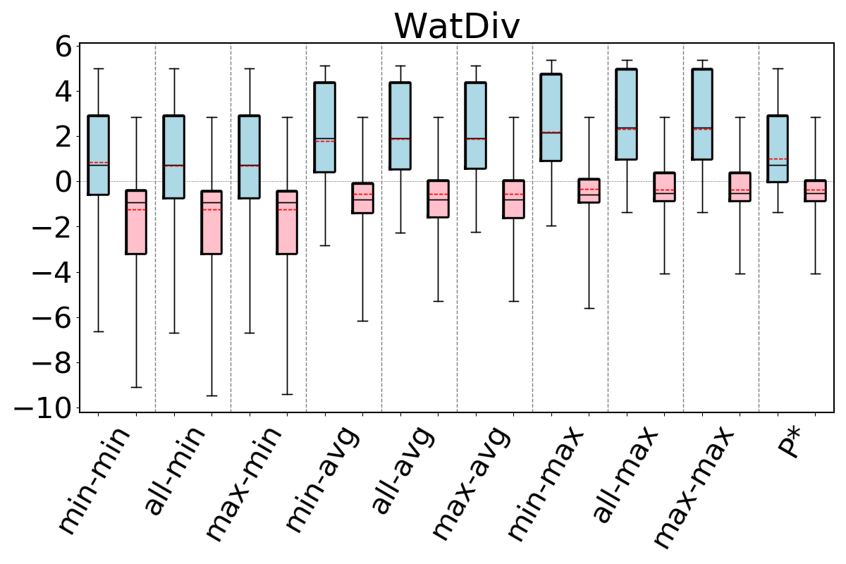
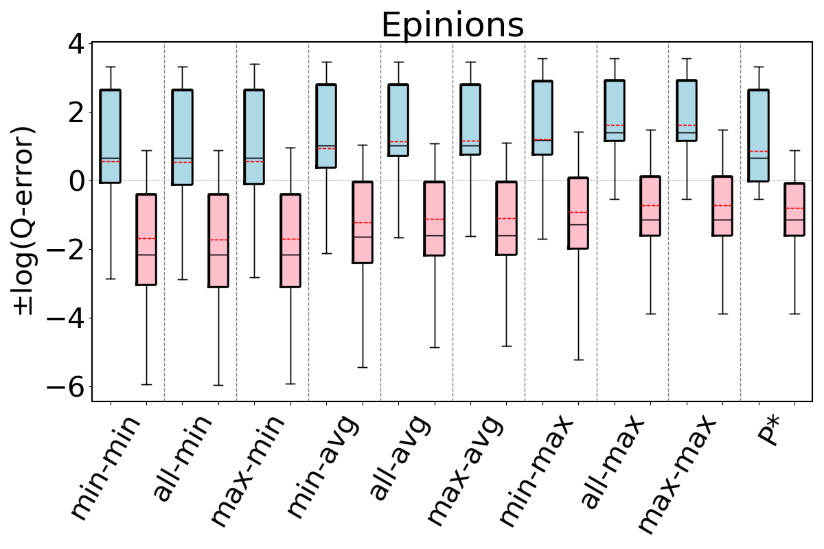
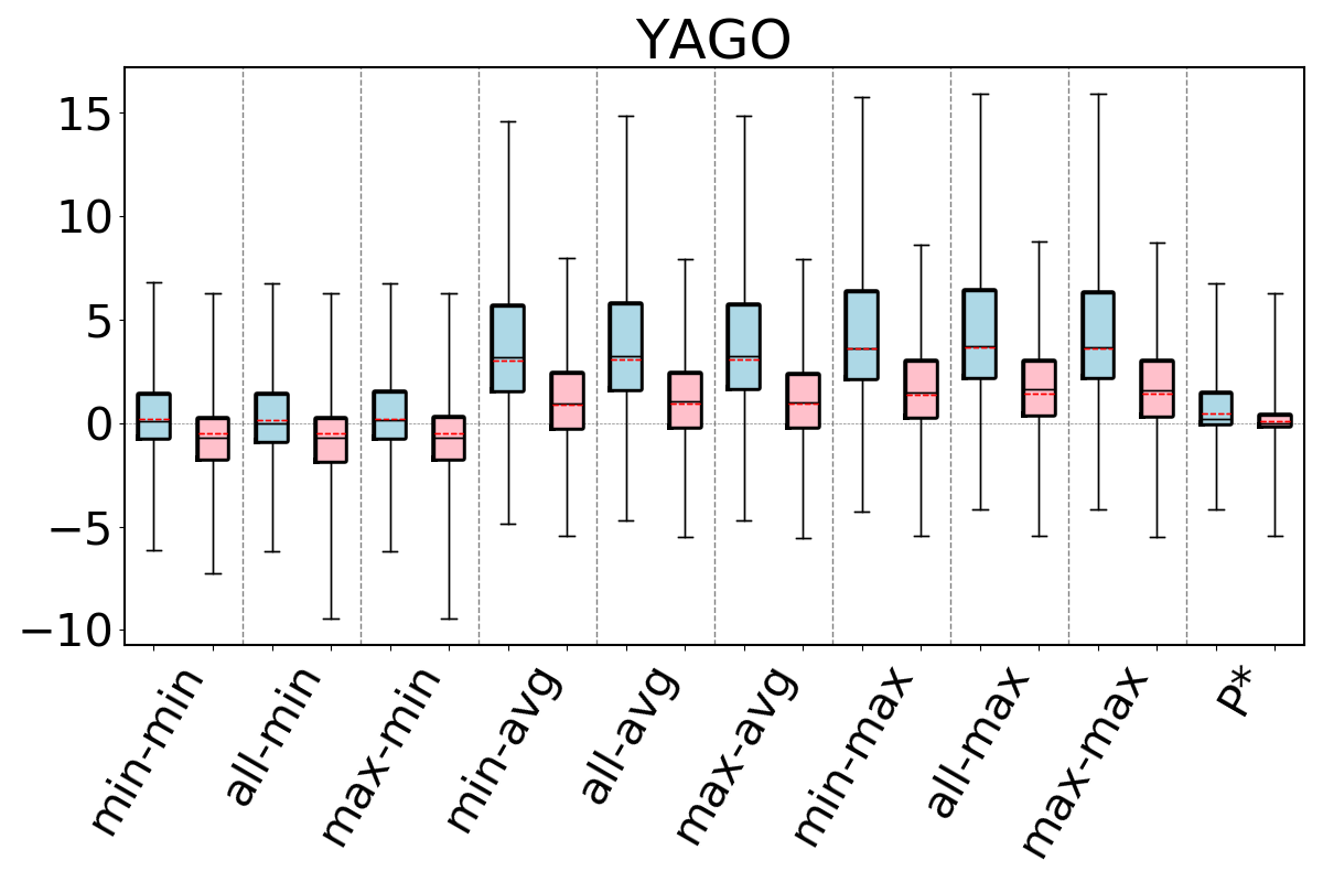
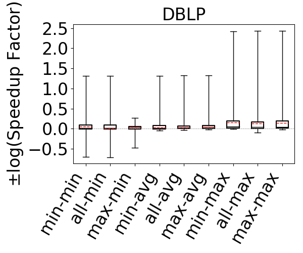
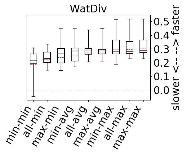
To compare the accuracies of different estimators, for each query in our workloads we make an estimate using each estimator and compute its q-error. If the true cardinality of is and the estimate is , then the q-error is . For each workload, this gives us a distribution of q-errors, which we compare as follows. First, we take the logs of the q-errors so they are now . If a q-error was an underestimate, we put a negative sign to it. This allows us to order the estimates from the least accurate underestimation to the least accurate overestimation. We then generate a box plot where the box represents the 25th, median, and 75th percentile cut-off marks. We also compute the mean of this distribution, excluding the top 10% of the distribution (ignoring under/over estimations) and draw it with a red dashed line in box plots.
6.2.1. Acyclic Queries and Cyclic Queries With Only Triangles
For our first question, we first compare our 9 estimators on for each acyclic query workload in our setup. We then compare our 9 estimators on each cyclic query workload, but only using the queries that only contain triangles as cycles. All except one clique-6 query in the GCARE-Cyclic workload contained cycles with more than 3 edges, so the YAGO-GCARE-Cyclic combination is omitted.
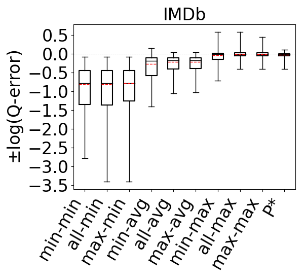
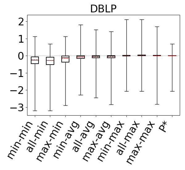
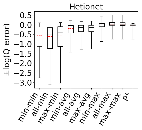
The accuracies of the 9 estimators on acyclic workloads are shown in Figure 9 (ignore the P* column for now). We make several observations. First, regardless of the path-length heuristic chosen, the max aggregator (the last 3 box plots in the figures) makes significantly more accurate estimates (note that the y-axis on the plots are in log scale) than avg, which in turn is more accurate than min. This is true across all acyclic experiments and all datasets. For example, on IMDb and JOB workload, the all-hops-min, all-hops-avg, and all-hops-max estimators have log of mean q-errors (after removing top 10 percent outliers) of 6.5 (underestimation), 1.7 (underestimation), and 1.02 (understimation), respectively. Overall, we observe that using the most pessimistic of the optimistic estimates leads to significantly more accurate estimations in our evaluations than the heuristics used in prior work (up to three orders of magnitude improvement in mean accuracy). Therefore on acyclic queries, when there are multiple formulas that can be used for estimating a query’s cardinality, using the pessimistic ones is an effective technique to combat the well known underestimation problem.
We next analyze the path-length heuristics. Observe that across all experiments, if we ignore the outliers and focus on the 25-75 percentile boxes, max-hop and all-hops do at least as well as min-hop. Further observe that on IMDb, Hetionet, and on the Acyclic workload on Epinions, max-hop and all-hops lead to significantly more accurate estimates. Finally, the performance of max-hop and all-hops are comparable across our experiments. We verified that this is because all-hops effectively picks one of the max-hop paths in majority of the queries in our workloads. Since max-hop enumerates strictly fewer paths than all-hops to make an estimate, we conclude that on acyclic queries, systems implementing the optimistic estimators can prefer the max-hop-max estimator.
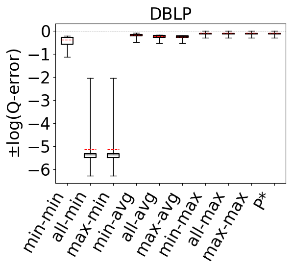
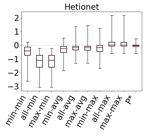
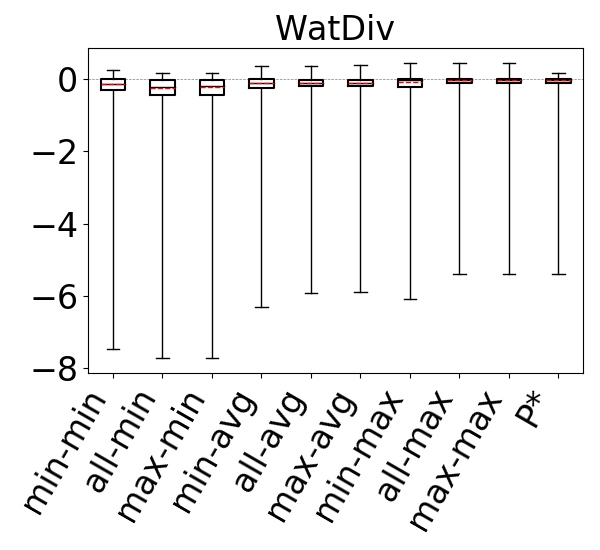
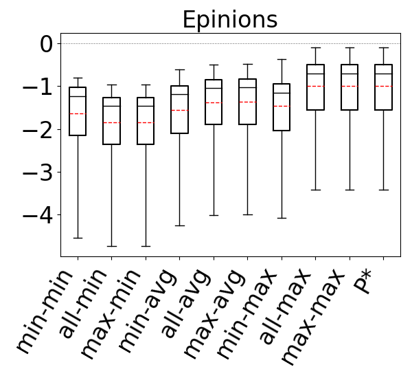
Figure 10 shows the accuracies of the 9 estimators on cyclic query workloads with only triangles. Our observations are similar to those for acyclic queries, and we find that the max aggregator yields more accurate estimates than other aggregators, irrespective of the path length. This is again because we generally observe that on most datasets any of the 9 estimators tend to underestimate, and the max aggregator can combat this problem better than min or avg. When using the max aggregator, we also observe that the max-hop heuristic performs at least as well as the min-hop heuristic. Therefore, as we observed for acyclic queries, we find max-hop-max estimator to be an effective way to make accurate estimations for cyclic queries with only triangles.
For the above experiments, we also performed a query template-specific analysis and verified that our conclusions generally hold for each acyclic and cyclic query template we used in our workloads in Figures 9 and 10. Our charts in which we evaluate the 9 estimators on each query template can be found in our github repo.

6.2.2. Cyclic Queries With Cycles of Size 3
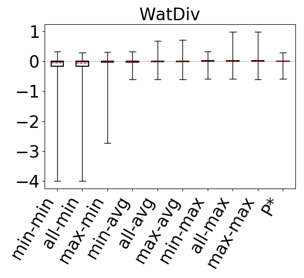
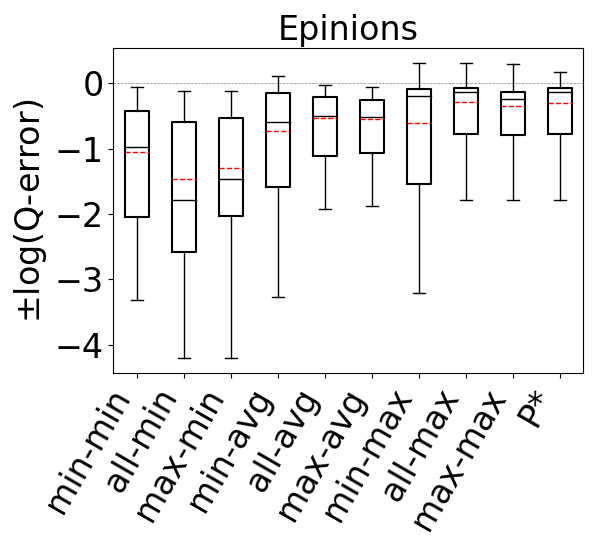
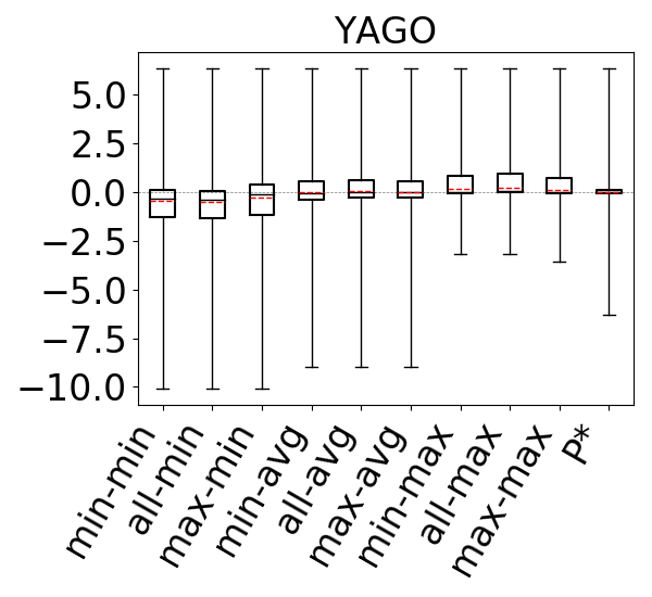
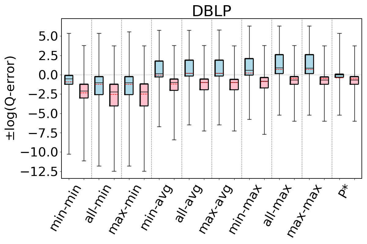
For our second question, we compare our 9 estimators on and for each dataset-cyclic query workload combination in our benchmark, but only using queries that contain cycles of size . Recall that we now expect that estimates on can be generally pessimistic. This is because any formula (or bottom to top path) in breaks large cycles and estimates paths and on real world datasets there are often a lot more paths than cycles. In contrast, we expect the edge weights in to fix this pessimism, so estimates on these CEGs can still be optimistic. Figure 11 shows our results. As we expected, we now see that across all of the datasets, our 9 estimators on generally overestimate. In contrast to our observations for acyclic queries and cyclic queries with only cycles, we now see that the most accurate results are achieved when using the min aggregator (instead of max). For the min aggregator, any of the path-length heuristics seem to perform reasonably well. On DBLP we see that the min-hop-min heuristic leads to more accurate results, while on Hetionet max-hop and all-hops heuristics, and results are comparable in other datasets.
In contrast, on , similar to our results from Figures 9 and 10, we still observe that max aggregator yields more accurate results, although the avg aggregator also yields competitive results on Hetionet and YAGO. This shows that simulating the cycle closing by using cycle closing rates avoids the pessimism of and results in optimisitic estimates. Therefore, as before, countering this optimism using the pessimistic paths in is an effective technique to achieve accurate estimates. In addition, we also see that any of the path-length heuristics perform reasonably well.
Finally to answer our third question, we compare , and under their best performing heuristics. We take as this estimator min-hop-min for and max-hop-max for . We see that, except for DBLP and YAGO where the estimates are competitive, the estimates on are more accurate. For example, on Hetionet, while the median q-error for min-hop-min on is 213.8 (overestimation), it is only 2.0 (overestimation) for max-hop-max . Therefore, we observe that even using the most optimistic estimator on may not be very accurate on cyclic queries with large cycles and modifying this CEG with cycle closing rates can fix this shortcoming.
6.2.3. Estimator and Room for Improvement
We next answer the question of how much room for improvement there is for the space of optimistic estimators we considered on and . To do so, we consider a thought experiment in which, for each query in our workloads, an oracle picks the most accurate path in our CEGs. The accuracies of this oracle-based estimator are shown as bars in our bar charts in Figures 9-11. We compare the bars in these figures with the max-hop-max estimator on on acyclic queries and cyclic queries with only triangles, and max-hop-max estimator on for queries with larger cycles. We find that on acyclic queries, shown in Figure 9, we generally see little room for improvement, though there is some room in Hetionet and YAGO. For example, although the median q-errors of max-hop-max and are indistinguishable on Hetionet, the 75 percentile cutoffs for max-hop-max and are 1.52 and 1.07, respectively. We see more room for improvement on cyclic query workloads that contain large cycles, shown in Figures 11. Although we still find that on DBLP, WatDiv and Epinions, max-hop-max estimator on is competitive with , there is a more visible room for improvement on Hetionet and YAGO. For example, on Hetionet, the median q-errors of max-hop-max and are 1.48 (overestimation) and 1.02 (underestimation), respectively. On YAGO the median q-errors are 39.8 (overestimation) and 1.01 (overestimation), respectively. This indicates that future work on designing other techniques for making estimations on CEG-based estimators can focus on workloads with large cycles on these datasets to find opportunities for improvement.
6.3. Effects of Bound Sketch
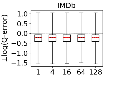
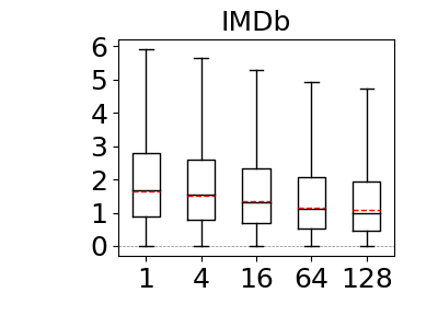
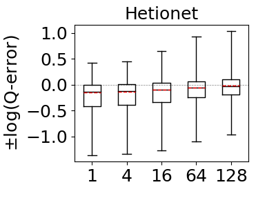
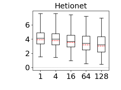
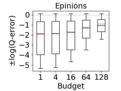
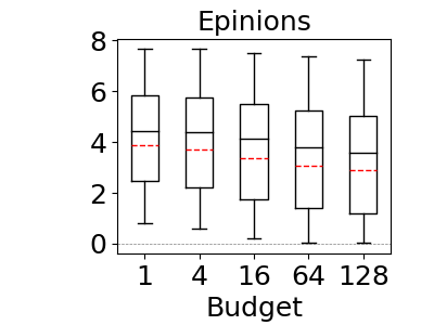
Our next set of experiments aim to answer: How much does the bound-sketch optimization improve the optimistic estimators’ accuracy? This question was answered for the CBS pessimistic estimator in reference (Cai et al., 2019). We reproduce the experiment for MOLP in our context as well. To answer this question, we tested the effects of bound sketch on the JOB workload on IMDb and Acyclic workload on Hetionet and Epinions. We excluded WatDiv and DBLP as the max-hop-max estimator’s estimates are already very close to perfect on these datasets and there is no room for significant improvement (recall Figure 9). Then we applied the bound sketch optimization to both max-hop-max (on ) and MOLP estimators and measured the q-errors of the estimators under partitioning budgets of 1 (no partitioning), 4, 16, 64, and 128.
Our results are shown in Figure 12. As demonstrated in reference (Cai et al., 2019), our results confirm that bound sketch improves the accuracy of MOLP. The mean accuracy of MOLP increases between 15% and 89% across all of our datasets when moving between 1 and 128 partitions. Similarly, we also observe significant gains on the max-hop-max estimator though the results are data dependent. On Hetionet and Epinions, partitioning improves the mean accuracy at similar rates: by 25% and 89%, respectively. In contrast, we do not observe significant gains on IMDb. We note that the estimations of 68% of queries in Hetionet and 93% in Epinions strictly improved, so bound sketch is highly robust for optimistic estimators. We did not observe significant improvements in IMDb dataset for max-hop-max, although 93% of their q-errors strictly improve, albeit by a small amount. We will compare optimistic and pessimistic estimators in more detail in the next sub-section but readers can already see by inspecting the scale in the y-axes of Figure 12 that as observed in reference (Park et al., 2020) the pessimistic estimators are highly inaccurate and in our context orders of magnitude less accurate than optimistic ones.
6.4. Summary-based Estimator Comparison
The optimistic and pessimistic estimators we consider in this paper are summary-based estimators. Our next set of experiments compares max-hop-max (on ) and MOLP against each other and against other baseline summary-based estimators. A recent work (Park et al., 2020) has compared MOLP against two other summary-based estimators, Characteristic Sets (CS) (Neumann and Moerkotte, 2011) and SumRDF (Stefanoni et al., 2018). We reproduce and extend this comparison in our setting with our suggested max-hop-max optimistic estimator. We first give an overview of CS and SumRDF.
CS: CS is a cardinality estimator that was used in the RDF-3X system (Neumann and Weikum, 2008). CS is primarily designed to estimate the cardinalities of stars in an RDF graph. The statistic that it uses are based on the so-called characteristic set of each vertex in an RDF graph, which is the set of distinct outgoing labels has. CS keeps statistics about the vertices with the same characteristic set, such as the number of nodes that belong to a characteristic set. Then, using these statistics, the estimator makes estimates for the number of distinct matches of stars. For a non-star query , is decomposed into multiple stars , and the estimates for each is multiplied, which corresponds to an independence assumption.
SumRDF: SumRDF builds a summary graph of an RDF graph and adopts a holistic approach to make an estimate. Given the summary , SumRDF considers all possible RDF graphs that could have the same summary . Then, it returns the average cardinality of across all possible instances. This is effectively another form of uniformity assumption: each possible world has the same probability of representing the actual graph on which the estimate is being made. Note that the pessimistic estimators can also be seen as doing something similar, except they consider the most pessimistic of the possible worlds and return the cardinality of on that instance.
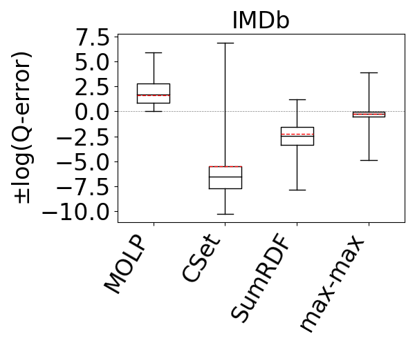
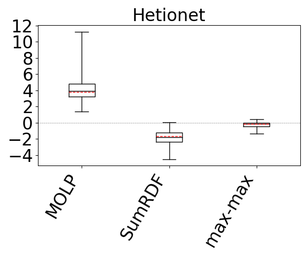
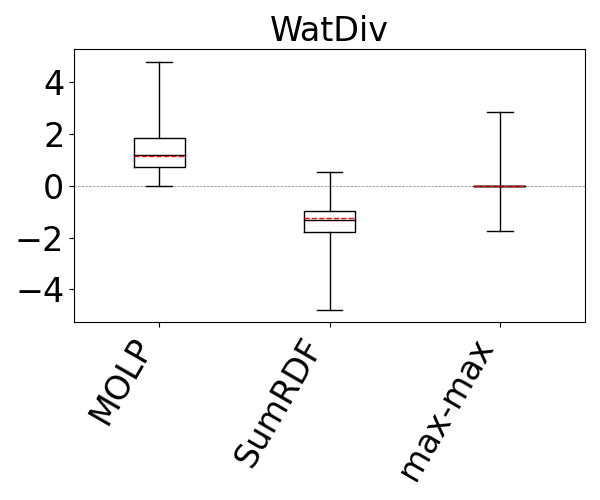
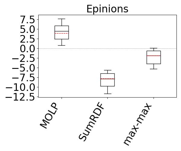
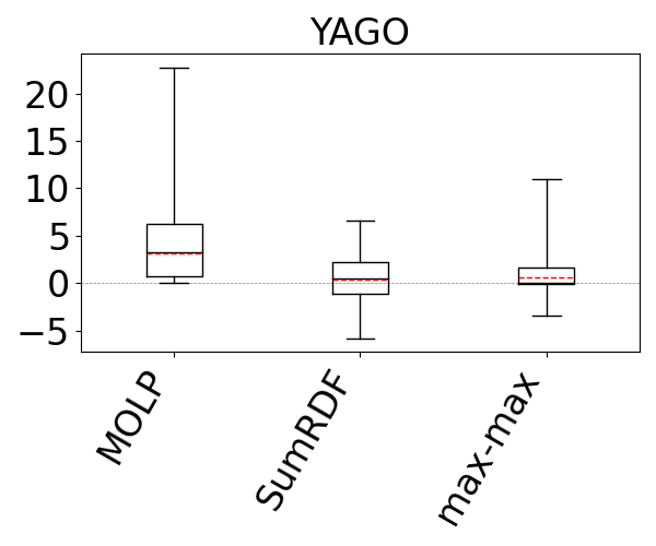
We measured the q-errors of max-hop-max, MOLP, CS, and SumRDF on the JOB workload on IMDb, the Acyclic workload on Hetionet, WatDiv, and Epinions, and the G-CARE-Acyclic workload on YAGO. We did not use bound sketch for MOLP and max-hop-max. However, we ensured that MOLP uses the cardinalities and degree information from 2-size joins, which ensures that the statistics MOLP uses is a strict superset of the statistics max-hop-max estimator uses.
Our results are shown in Figure 13. We omit CS from all figures except the first one, because it was not competitive with the rest of the estimators and even when y-axis is in logarithmic scale, plotting CS decreases the visibility of differences among the rest of the estimators. SumRDF timed out on several queries on YAGO and Hetionet and we removed those queries from max-hop-max and MOLP’s distributions as well. We make two observations. First, these results confirm the results from reference (Park et al., 2020) that although MOLP does not underestimate, its estimates are very loose. Second, across all summary-based estimators, unequivocally, max-hop-max generates significantly more accurate estimations, often by several orders of magnitude in mean estimation. For example, on the IMDb and JOB workload, the mean q-errors of max-hop-max, SumRDF, MOLP, and CS are 1.8, 193.3, 44.6, and 333751, respectively. We also note that both CS and SumRDF perform underestimations in virtually all queries, whereas there are datasets, such as WatDiv and YAGO, where the majority of max-hop-max’s estimates are overestimations.
6.5. Comparison Against WanderJoin
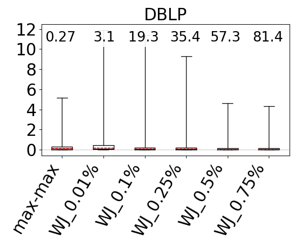
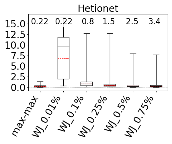
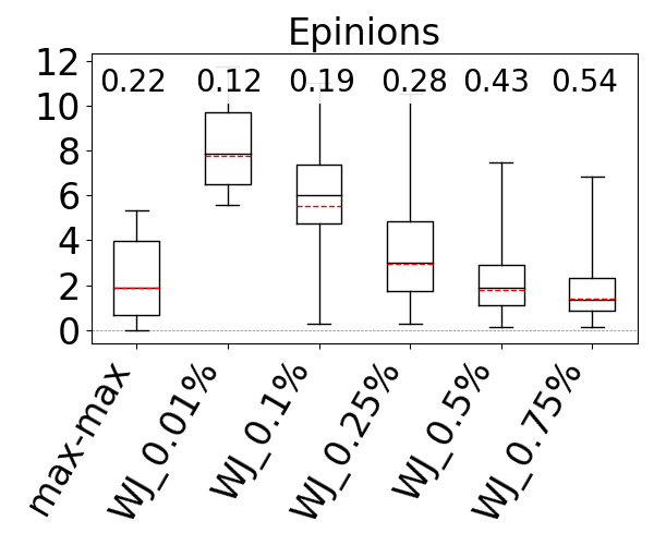
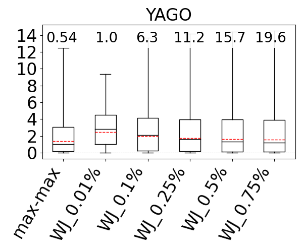
Although we studied summary-based estimators in this paper, an alternative technique that has been studied is based on sampling. Sampling-based techniques are fundamentally different and based on using unbiased samplers of the query’s output. As such, their primary advantage is that by enough sampling they are guaranteed to achieve estimations at any required accuracy. However, because they effectively perform the join on a sample of tuples, they can be slow, which is why they have seen little adoption in practice for join estimation. This time-vs-accuracy tradeoff is fundamentally different in summary-based estimators, which can give more accurate estimates only by storing more statistics, (e.g., larger join-sizes in Markov tables), so with more memory and not time. For completeness of our work, we compare max-hop-max estimator with WanderJoin (WJ) (Li et al., 2016; Park et al., 2020), which is a sampling-based estimator that was identified in reference (Park et al., 2020) as the most efficient sampling-based technique out of a set of techniques the authors experimented with. Our goal is to answer: What is the sampling ratio at which WJ’s estimate outperforms max-hop-max (on ) in accuracy and how do the estimation speeds of WJ and max-hop-max compare at this ratio? We first give an overview of WJ as implemented in reference (Park et al., 2020).
WanderJoin: WJ is similar to the index-based sampling described in reference (Leis et al., 2017). Given a query , WJ picks one of the query edges of to start the join from and picks a sampling ratio , which is the fraction of edges that can match that it will sample. For each sampled edge (with replacement), WJ computes the join one query-edge at-a-time by picking one of the possible edges of a vertex that has already been matched uniformly at random. Then, if the join is successfully computed, a correction factor depending on the degrees of the nodes that were extended is applied to get an estimate for the number of output results that would extend to. Finally, the sum of the estimates for each sample is multiplied by to get a final estimate.
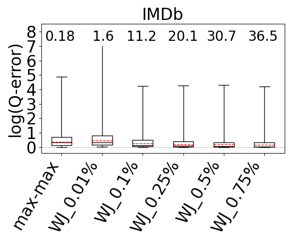
We used the G-CARE’s codebase (Park et al., 2020). We integrated the max-hop-max estimator into G-CARE and used the WJ code that was provided. We compared WJ and max-hop-max with sampling ratios 0.01%, 0.1%, 0.25%, 0.5%, and 0.75% on the JOB workload on IMDb, the Acyclic workload on Hetionet, WatDiv, and Epinions, and the G-CARE-Acyclic workload on YAGO. We ran both estimators five times (each run executes inside a single thread) and report the averages of their estimation times. We also report the average q-error of WJ. However, we can no longer present under- and over-estimations in our figures, as WJ might under and over-estimate for the same query across different runs.
The box-plot q-error distributions of max-hop-max and WJ are shown in Figure 14. We identify the sampling ratios in which the mean accuracy of WJ is better than the mean accuracy of max-hop-max, except in DBLP and Hetionet, where both max-hop-max and WJ’s mean estimates are generally close to perfect, so we look at the sampling ratio where WJ’s maximum q-errors are smaller than max-hop-max. We find that this sampling ratio on IMDb is 0.1%, on DBLP is 0.5%, on Hetionet is 0.75%, on Epinions is 0.5%, and on YAGO is 0.75%. However, the estimation time of WJ is between 15x and 212x slower, so one to two orders of magnitude, than max-hop-max except on our smallest dataset Epinions, where the difference is 1.95x. Observe that max-hop-max’s estimation times are very stable and consistently in sub-milliseconds, between 0.18ms and 0.54ms. This is because max-hop-max’s estimation time is independent of the dataset’s size. In contrast, WJ’s estimation times get slower as the datasets get larger, because WJ performs more joins. For example, at 0.25% ratio, while WJ takes 0.28ms on our smallest dataset Epinions, it takes 35.4ms on DBLP.
We emphasize that these comparisons are not perfect because it is difficult to compare distributions and these are two fundamentally different classes of estimators, providing systems with different tradeoffs. However, we believe that our ‘competitive sampling ratio’ analysis (more than runtime numbers) is instructive for interested readers.
6.6. Impact on Plan Quality
Reference (Leis et al., 2015) convincingly established that cardinality estimation is critical for optimizers to generate good plans for RDBMSs as it leads to better plan generation. Several other work has verified this in different contexts, in RDBMSs (Cai et al., 2019) and in RDF systems (Park et al., 2020). In our final set of experiments we set out to verify this in our context too by comparing the impact of our estimators on plan quality. We used the RDF-3X system (Neumann and Weikum, 2008) and its source code available here (rdf3x, 2020). We issued our Acyclic workload as join-only queries to RDF-3X on the DBLP and WatDiv datasets. We then ran the query under 10 configurations: first using RDF-3X’s default estimator and then by injecting the cardinality estimates of our 9 optimistic estimators to the system. The cardinalities are injected inside the system’s dynamic programming-based join optimizer. We then filtered out the queries in which all of the 10 estimators lead to picking exactly the same plan and there was less than 10% runtime difference between the minimum and maximum runtimes across the plans generated from 10 estimators. We were left with 15 queries for DBLP and 8 queries for WatDiv. We ran each query times and report the best query execution time. The open source version of RDF-3X uses a simple cardinality estimator that is not based on characteristic sets as in reference (Neumann and Weikum, 2008) but on basic statistics about the original triple counts and some ‘magic’ constants to estimate cardinalities. We observed that this estimator is highly inaccurate compared to the 9 optimistic estimators. For example, we analyzed the final estimates of the RDF-3X estimator on the 8 WatDiv queries and compared with the other estimators. We omit the full results but while the RDF-3X estimator had a median q-error of 127.4 underestimation, the worst-performing of the 9 estimators had a median q-error of only 1.947 underestimation. So we expect RDF-3X’s estimator to lead to worse plans than the other estimators. We further expect generally that the more accurate of the optimistic estimators, such as the max-hop-max estimator, yield more efficient plans than the less accurate ones, such as the min-hop-min.
Figure 15 shows the runtimes of the system under each configuration where the y-axis shows the log-scale speedup or slow down of each plan under each estimator compared to the plans under the RDF-3X estimator. This is why the figure does not contain a separate box plot for the RDF-3X estimator. First observe that the median lines of the 9 estimators are above 0, indicating the each of these estimators, which have more accurate estimates than RDF-3X’s default estimator, leads to better plan generation. In addition, observe that the box plot of estimators with the max aggregators are generally better than estimators that use the min or avg aggregator. This correlates with Figure 9, where we showed these estimators lead to more accurate estimations on the same set of queries. We then performed a detailed analysis of the max-hop-max and min-hop-min estimator as representative of, respectively, the most and least accurate of the 9 estimators. We analyzed the queries in which plans under these estimators differed significantly. Specifically, we found 10 queries across both datasets where the runtime differences were at least 1.15x. Of these, only in 1 of them min-hop-min lead to more efficient plans and by a factor of 1.21x. In the other 9, max-hop-max lead to more efficient plans, by a median of 2.05x and up to 276.3x, confirming our expectation that better estimations generally lead to better plans.
7. Related Work
There are decades of research on cardinality estimation of queries in the context of different database management systems. We cover a part of this literature focusing on work on graph-based database management systems, specifically XML and RDF and on relational systems. We covered Characteristic Sets (Neumann and Moerkotte, 2011), SumRDF (Stefanoni et al., 2018), and WanderJoin (Li et al., 2016; Park et al., 2020) in Section 6. We cover another technique, based on maximum entropy that can be used with any estimator that can return estimates for base tables or small-size joins. We do not cover work that uses machine learning techniques to estimate cardinalities and refer the reader to several recent work in this space (Kipf et al., 2019; Liu et al., 2015; Woltmann et al., 2019) for details of these techniques.
Other Summary-based Estimators: The estimators we studied in this paper fall under the category of summary-based estimators. Many relational systems, including commercial ones such as PostgreSQL, use summary-based estimators. Example summaries include the cardinalities of relations, the number of distinct values in columns, or histograms (Aboulnaga and Chaudhuri, 1999; Muralikrishna and DeWitt, 1988; Poosala and Ioannidis, 1997), wavelets (Matias et al., 1998), or probabilistic and statistical models (Getoor et al., 2001; Sun et al., 1993) that capture the distribution of values in columns. These statistics are used to estimate the selectivities of each join predicate, which are put together using several approaches, such as independence assumptions. In contrast, the estimators we studied store degree statistics about base relations and small-size joins (note that cardinalities are a form of degree statistics, e.g., ).
Several estimators for subgraph queries have proposed summary-based estimators that compute a sketch of an input graph. SumRDF, which we covered in Section 6, falls under this category. In the context of estimating the selectivities of path expressions, XSeed (Zhang et al., 2006) and XSketch (Polyzotis and Garofalakis, 2002) build a sketch of the input XML Document. The sketch of the graph effectively collapses multiple nodes and edges into supernodes and edges with metatadata on the nodes and edges. The metadata contains statistics, such as the number of nodes that was collapsed into a supernode. Then given a query , is matched on and using the metadata an estimate is made. Because these techniques do not decompose a query into smaller sub-queries, the question of which decomposition to use does not arise for these estimators.
Several work have used data structures that are adaptations of histograms from relational systems to store selectivities of path or tree queries in XML documents. Examples include, positional histograms (Wu et al., 2002) and Bloom histogram (Wang et al., 2004). These techniques do not consecutively make estimates for larger paths and have not been adopted to general subgraph queries. For example, instead of storing small-size paths in a data structure as in Markov tables, Bloom histograms store all paths but hashed in a bloom filter. Other work used similar summaries of XML documents (or its precursor the object exchange model (Papakonstantinou et al., 1995) databases) for purposes other than cardinality estimation. For example, TreeSketch (Polyzotis et al., 2004) produces a summary of large XML documents to provide approximate answers to queries.
Sampling-based Estimators: Another class of important estimators are based on sampling tuples (Haas, Peter J. and Naughton, Jeffrey F. and Seshadri, S. and Swami, Arun N., 1996; Leis et al., 2017; Li et al., 2016; Vengerov et al., 2015; Wu et al., 2016). These estimators either sample input records from base tables offline or during query optimization, and they evaluate queries on these samples to make estimates. Research has focused on different ways samples can be generated, such as independent or correlated sampling, or sampling through existing indexes. Wander Join, which we covered in Section 6 falls under this category. As we discussed, by increasing the sizes of the samples these estimators can be arbitrarily accurate but they are in general slower than summary-based ones because they actually perform the join on a sample of tuples. We are aware of systems (Leis et al., 2018) that use sampling-based estimators to estimate the selectivities of predicates in base tables but not on multiway joins. Finally, sampling-based estimators have also been used to estimate frequencies of subgraphs relative to each other to discover motifs, i.e. infrequently appearing subgrahs, (Kashtan et al., 2004).
The Maximum Entropy Estimator: Markl et al. (Markl et al., 2007) has proposed another approach to make estimates for conjunctive predicates, say given a set of selectivity estimates , , where is the selectivity estimate for predicate . Markl et al.’s maximum entropy approach takes these known selectivities and uses a constraint optimization problem to compute the distribution that maximizes the entropy of the joint distribution of the possible predicate space. Reference (Markl et al., 2007) has only evaluated the accuracy of this approach for estimating conjunctive predicates on base tables and not on joins, but they have briefly described how the same approach can be used to estimate the cardinalities of join queries. Multiway join queries can be modeled as estimating the selectivity of the full join predicate that contains the equality constraint of all attributes with the same name. The statistics that we considered in this paper can be translated to selectivities of each predicate. For example the size of can be modeled as , as the join of and is by definition applying the predicate predicate on the Cartesian product of relations and . This way, one can construct another optimistic estimator using the same statistics. We have not investigated the accuracy of this approach within the scope of this work and leave this to future work.
8. Conclusions and Future Work
We focused on how to make accurate estimations using the optimistic estimators using a new framework, in which we model these estimators as paths in a weighted CEG we called , which uses as edge weights average degree statistics. We addressed two shortcomings of optimistic estimators from prior work. First, we addressed the question of which formulas, i.e., CEG paths, to use when there are multiple formulas to estimate a given query. We outlined and empirically evaluated a space of heuristics and showed that the heuristic that leads generally to most accurate estimates depends on the structure of the query. For example, we showed that for acyclic queries and cyclic queries wth small-size cycles, using the maximum weight path is an effective way to make accurate estimates. Second, we addressed how to make accurate estimates for queries with large cycles by proposing a new CEG that we call . We then showed that surprisingly the recent pessimistic estimators can also be modeled as picking a path, this time the minimum weight path in another CEG, in which the edge weights are maximum degree statistics. Aside from connecting two disparate classes of estimators, this observation allowed us to apply the bound sketch optimization for pessimistic estimators to optimistic ones. We also showed that CEGs are useful mathematical tools to prove several properties of pessimistic estimators, e.g., that the CBS estimator is equivalent to MOLP estimator under acyclic queries over binary relations.
We believe the CEG framework can be the foundation for further research to define and evaluate other novel estimators. Within the scope of this work, we considered only three specific CEGs, with a fourth one that is used for theoretical purposes in Appendix D. However, many other CEGs can be defined to develop new estimators using different statistics and potentially different techniques to pick paths in CEGs as estimates. For example, one can use variance, standard deviation, or entropies of the distributions of small-size joins as edge weights in a CEG, possibly along with degree statistics, and pick the minimum-weight, e.g.,, “lowest entropy”, paths, assuming that degrees are more regular in lower entropy edges. An important research direction is to systematically study a class of CEG instances that use different combination of statistics as edge weights, as well as heuristics on these CEGs for picking paths, to understand which statistics lead to more accurate results in practice.
9. Acknowledgment
This work was supported by NSERC and by a grant from Waterloo-Huawei Joint Innovation Laboratory.
References
- (1)
- Abo Khamis et al. (2016) Mahmoud Abo Khamis, Hung Q. Ngo, and Dan Suciu. 2016. Computing Join Queries with Functional Dependencies. In PODS.
- Aboulnaga et al. (2001) Ashraf Aboulnaga, Alaa R. Alameldeen, and Jeffrey F. Naughton. 2001. Estimating the Selectivity of XML Path Expressions for Internet Scale Applications. In VLDB.
- Aboulnaga and Chaudhuri (1999) Ashraf Aboulnaga and Surajit Chaudhuri. 1999. Self-Tuning Histograms: Building Histograms Without Looking at Data. In SIGMOD.
- Atserias et al. (2013) A. Atserias, M. Grohe, and D. Marx. 2013. Size Bounds and Query Plans for Relational Joins. SICOMP 42, 4 (2013).
- Cai et al. (2019) Walter Cai, Magdalena Balazinska, and Dan Suciu. 2019. Pessimistic Cardinality Estimation: Tighter Upper Bounds for Intermediate Join Cardinalities. In SIGMOD.
- Getoor et al. (2001) Lise Getoor, Benjamin Taskar, and Daphne Koller. 2001. Selectivity Estimation Using Probabilistic Models. In SIGMOD.
- Gottlob et al. (2012) Georg Gottlob, Stephanie Tien Lee, Gregory Valiant, and Paul Valiant. 2012. Size and Treewidth Bounds for Conjunctive Queries. JACM 59, 3 (2012).
- Haas, Peter J. and Naughton, Jeffrey F. and Seshadri, S. and Swami, Arun N. (1996) Haas, Peter J. and Naughton, Jeffrey F. and Seshadri, S. and Swami, Arun N. 1996. Selectivity and Cost Estimation for Joins Based on Random Sampling. JCSS 52, 3 (1996).
- Joglekar and Ré (2018) Manas Joglekar and Christopher Ré. 2018. It’s All a Matter of Degree - Using Degree Information to Optimize Multiway Joins. TOCS 62, 4 (2018).
- Kashtan et al. (2004) Nadav Kashtan, Shalev Itzkovitz, Ron Milo, and Uri Alon. 2004. Efficient Sampling Algorithm for Estimating Subgraph Concentrations and Detecting Network Motifs. Bioinformatics 20, 11 (2004).
- Kipf et al. (2019) Andreas Kipf, Thomas Kipf, Bernhard Radke, Viktor Leis, Peter A. Boncz, and Alfons Kemper. 2019. Learned Cardinalities: Estimating Correlated Joins with Deep Learning. In CIDR.
- Leis et al. (2015) Viktor Leis, Andrey Gubichev, Atanas Mirchev, Peter Boncz, Alfons Kemper, and Thomas Neumann. 2015. How Good Are Query Optimizers, Really?. In VLDB.
- Leis et al. (2017) Viktor Leis, Bernhard Radke, Andrey Gubichev, Alfons Kemper, and Thomas Neumann. 2017. Cardinality Estimation Done Right: Index-Based Join Sampling. In CIDR.
- Leis et al. (2018) Viktor Leis, Bernhard Radke, Andrey Gubichev, Atanas Mirchev, Peter Boncz, Alfons Kemper, and Thomas Neumann. 2018. Query Optimization Through the Looking Glass, and What We Found Running the Join Order Benchmark. VLDBJ 27, 5 (2018).
- Li et al. (2016) Feifei Li, Bin Wu, Ke Yi, and Zhuoyue Zhao. 2016. Wander Join: Online Aggregation via Random Walks. In SIGMOD.
- Liu et al. (2015) Henry Liu, Mingbin Xu, Ziting Yu, Vincent Corvinelli, and Calisto Zuzarte. 2015. Cardinality Estimation Using Neural Networks. In CASCON.
- Maduko et al. (2008) Angela Maduko, Kemafor Anyanwu, Amit Sheth, and Paul Schliekelman. 2008. Graph Summaries for Subgraph Frequency Estimation. In ESWC.
- Markl et al. (2007) V. Markl, P. J. Haas, M. Kutsch, N. Megiddo, U. Srivastava, and T. M. Tam. 2007. Consistent Selectivity Estimation via Maximum Entropy. VLDBJ 16 (2007).
- Matias et al. (1998) Yossi Matias, Jeffrey Scott Vitter, and Min Wang. 1998. Wavelet-Based Histograms for Selectivity Estimation. In SIGMOD.
- Mhedhbi and Salihoglu (2019) Amine Mhedhbi and Semih Salihoglu. 2019. Optimizing Subgraph Queries by Combining Binary and Worst-Case Optimal Joins. PVLDB 12, 11 (2019).
- Muralikrishna and DeWitt (1988) M. Muralikrishna and David J. DeWitt. 1988. Equi-Depth Histograms for Estimating Selectivity Factors for Multi-Dimensional Queries. In SIGMOD.
- Neumann and Moerkotte (2011) Thomas Neumann and Guido Moerkotte. 2011. Characteristic Sets: Accurate Cardinality Estimation for RDF Queries with Multiple Joins. In ICDE.
- Neumann and Weikum (2008) Thomas Neumann and Gerhard Weikum. 2008. RDF-3X: A RISC-Style Engine for RDF. In VLDB.
- Papakonstantinou et al. (1995) Yannis Papakonstantinou, Hector Garcia-Molina, and Jennifer Widom. 1995. Object Exchange Across Heterogeneous Information Sources. In ICDE.
- Park et al. (2020) Yeonsu Park, Seongyun Ko, Sourav S. Bhowmick, Kyoungmin Kim, Kijae Hong, and Wook-Shin Han. 2020. G-CARE: A Framework for Performance Benchmarking of Cardinality Estimation Techniques for Subgraph Matching. In SIGMOD.
- Polyzotis and Garofalakis (2002) Neoklis Polyzotis and Minos Garofalakis. 2002. Statistical Synopses for Graph-Structured XML Databases. In SIGMOD.
- Polyzotis et al. (2004) Neoklis Polyzotis, Minos Garofalakis, and Yannis Ioannidis. 2004. Approximate XML Query Answers. In SIGMOD.
- Poosala and Ioannidis (1997) Viswanath Poosala and Yannis E. Ioannidis. 1997. Selectivity Estimation Without the Attribute Value Independence Assumption. In VLDB.
- rdf3x (2020) rdf3x 2020. RDF-3X Source Code. https://github.com/gh-rdf3x/gh-rdf3x/. (2020).
- Stefanoni et al. (2018) Giorgio Stefanoni, Boris Motik, and Egor V. Kostylev. 2018. Estimating the Cardinality of Conjunctive Queries over RDF Data Using Graph Summarisation. In WWW.
- Sun et al. (1993) Wei Sun, Yibei Ling, Naphtali Rishe, and Yi Deng. 1993. An Instant and Accurate Size Estimation Method for Joins and Selections in a Retrieval-Intensive Environment. In SIGMOD.
- Vengerov et al. (2015) David Vengerov, Andre Cavalheiro Menck, Mohamed Zait, and Sunil P. Chakkappen. 2015. Join Size Estimation Subject to Filter Conditions. In VLDB.
- Wang et al. (2004) Wei Wang, Haifeng Jiang, Hongjun Lu, and Jeffrey Xu Yu. 2004. Bloom Histogram: Path Selectivity Estimation for XML Data with Updates. In VLDB.
- Woltmann et al. (2019) Lucas Woltmann, Claudio Hartmann, Maik Thiele, Dirk Habich, and Wolfgang Lehner. 2019. Cardinality Estimation with Local Deep Learning Models. In aiDM.
- Wu et al. (2016) Wentao Wu, Jeffrey F. Naughton, and Harneet Singh. 2016. Sampling-Based Query Re-Optimization. In SIGMOD.
- Wu et al. (2002) Yuqing Wu, Jignesh M. Patel, and H. V. Jagadish. 2002. Estimating Answer Sizes for XML Queries. In EDBT.
- Yu and Ozsoyoglu (1979) C. T. Yu and M. Z. Ozsoyoglu. 1979. An Algorithm for Tree-query Membership of a Distributed Query. In COMPSAC.
- Zhang et al. (2006) Ning Zhang, M. Tamer Ozsu, Ashraf Aboulnaga, and Ihab F. Ilyas. 2006. XSEED: Accurate and Fast Cardinality Estimation for XPath Queries. In ICDE.
Appendix A Projection Inequalities Can Be Removed From MOLP
Consider any path … and consider its first projection edge, say . We show that we can remove and replace the rest of the edges to with (possibly) new edges to with exactly the same weights and construct … …., where , …, . This can be seen inductively as follows. We know because is a projection edge. Then if edge was an extension edge that extended to attributes, then by construction, there is another edge in with the same weight as . If instead was a projection edge that removed a set of attributes from , similarly there is another projection edge that removes the same set of attributes from . So inductively, we can find an alternative sub-path from to , … with the same length as the sub-path ….
Appendix B CBS Estimator’s Connection to MOLP On Acyclic Queries
We first show that on acyclic queries MOLP is at least as tight as the CBS estimator. Our proof is based on showing that for each bounding formula generated by BFG and FCG (respectively, Algorithms 1 and 2 in reference (Cai et al., 2019)), there is a path in . For a detailed overview of these algorithms, we refer the reader to reference (Cai et al., 2019). We then show that if the queries are further on binary relations, then the standard MOLP bound, which only contains degree statistics about subsets of attributes in each relation, is exactly equal to the CBS estimator.
For each bounding formula generated by BFG and FCG, there is a path in : Let be a coverage combination enumerated by FCG. Consider a bounding formula . We can represent as a set of triples, where is the set of attributes that covers and is of size either 0, , or . Let . Then the bounding formula generated for will have exactly cost (recall that ). This is because there are 3 cases: (i) if , then the BFG ignores and ; (ii) if , then BFG uses in its formula the degree of the single uncovered attribute in , which is equal to as only contains ; and (iii) if , then BFG uses in its formula, and since , .
We next show that contains an path with exactly the same weight as the cost of . We first argue that if is acyclic, then there must always be at least one relation in the coverage , that covers all of its attributes. Assume for the purpose of contradiction that each relation either covers 0 attributes or attributes. Then start with any that covers attributes. Let be the attribute not covered by . Then another relation must be covering but not covering exactly one attribute . Similarly a third relation must be covering but not covering another attribute , etc. Since the query is finite, there must be a relation that covers an and whose other attributes are covered by some relation , where , which forms a cycle, contradicting our assumption that is acyclic.
We can finally construct our path in . Let’s divide the relations into , which cover all of their attributes, i.e., , and , which cover all but one of their attributes, . We ignore the relations that do not cover any attributes. Let relation in and those in . Then we can construct the following path. The first of the path uses the cardinalities or relations in in an arbitrary order to extend to . For example this path can be: . Now to extend to , observe that for each uncovered attribute , there must be some relation , such that all of the attributes are already bound in . This is because and if each has at least 2 attributes in , then must be cyclic. Note that this is true because by definition of acyclicity (Yu and Ozsoyoglu, 1979) any “ear” that we remove can be iteratively covered by at most one relation, which means by the time we remove the last ear, we must be left with a relation and one attribute, which contradicts that had at least 2 uncovered attributes in . So we can iteratively extend the path with one attribute at a time with an edge of weight until we reach . Note that this path’s length would be exactly the same as the cost of the bounding formula generated by BFG and FCG for the coverage .
When relations of an acyclic query are binary the CBS estimator is equal to MOLP: Ideally we would want to prove that when relations are binary that any path in corresponds to a bounding formula. However this is not true. Consider the simple join . contains the following path, . There is no bounding formula corresponding to this path in the CBS estimator because the first edge with weight uses the cardinality of projection of . However, the CBS estimator does not use cardinalities of projections in its bounding formulas and only uses the cardinalities of relations. Instead, what can be shown is that if a path in uses the cardinalities of projections, then there is another path with at most the same length, for which the CBS estimator has a bounding formula.
First we show that given an acyclic query over binary relations, if a path in contains cardinalities of projections, then there is an alternative path that has at most the length of and that contains at least one more edge that uses the cardinality of a full relation. We assume w.l.o.g. that is connected. Note that in any edge from in must be using the cardinality of a relation or a projection of a relation (the only outgoing edges from are these edges). Let us divide the edge in into multiple groups: (i) are those edge that extend a subquery with two attributes and use the cardinality of a relation; (ii) are those edges that bound an attribute in a relation in and extend a subquery to one new attribute using the degree of in ; (iii) are those edges that extend a subquery by a single attribute , without bounding any attributes in the subquery, i.e., using the cardinality of the projection of a relation onto (so the weight of these edges look like ; and (iv) are the remaining edges that extend a subquery by one attribute either bounding another attribute in or some other attribute in .
We first note that we can assume w.l.o.g., that if any relation is used in an edge to extend to, say, , then cannot be an attribute covered by the edges in or . Otherwise we can always replace , which has weight with an edge we can classify as with weight because . Next, we argue that we can iteratively remove two edges from and possibly and instead add one edge to without increasing the length of . First observe that if is empty, we must have a relation whose both attributes are in set , in which case, we can remove these two edges and replace with a single edge that simply has weight and reduce ’s length because . Note that if is not empty, then at least one of the edges must be bounding an attribute and extending to using a relation , where must be extended by an edge in using the same relation . Otherwise there would be some edge in that extended a subquery to without bounding the attribute that appears in the weight of . This is because note that if we remove the relations that were used in the edges in and then we would be left with an acyclic query, so have relations and attributes that need to be covered by and . If no edge is bounding an attribute in , then one of the relations must appear twice in the edges in , which cannot happen because the relations are binary (i.e., this would imply that the attributes of a relation were covered with two edges with weights and , which cannot happen). Therefore such an and must exist. Then we can again remove them and replace with one edge to with weight and decrease the weight of . Therefore from any we can construct a whose length is at most and that only consist of edges and . Readers can verify that each such path directly corresponds to a bounding formula generated by BFG and FCG (each relation used by an edge in and , respectively corresponds to a relation covering exactly and attributes).
Appendix C Counter Example for Using the CBS Estimator on Cyclic Queries
Consider the triangle query . FCG would generate the cover , , and . For this cover, BFG would generate the bounding formula: , which may not be a pessimistic bound. As an example, suppose each relation , , and contains tuples of the form . Then this formula would generate a bound of 0, whereas the actual number of triangles in this input is .
Appendix D DBPLP
We demonstrate another application of CEGs and provide alternative combinatorial proofs to some properties of DBPLP, which is another worst-case output size bound from reference (Joglekar and Ré, 2018). DBPLP is not as tight as MOLP, which our proofs demonstrate through a path-analysis of CEGs. We begin by reviewing the notion of a cover of a query.
Definition 1.
A cover is a set of (, ) pairs where and , such that the union of in “cover” all of , i.e., .
DBPLP of a query is defined for a given cover as follows:
Note that unlike MOLP, DBPLP is a maximization problem and has one variable for each attribute (instead of each subset of ). Similar to the MOLP constraints, we can also provide an intuitive interpretation of the DBPLP constraints. For any and , let . Each constraint of the DBPLP indicates that the number of ’s that any tuple that contains can extend to is , which is the maximum degree of any value in . Each constraint is therefore effectively an extension inequality using a maximum degree constraint. Based on this interpretation, we next define a DBPLP CEG, , to provide insights into DBPLP.
DBPLP CEG ():
-
Vertices: For each we have a vertex.
-
Extension Edges: Add an edge with weight between any and , such that and .
We note that DBPLP is not the solution to some path in this CEG, but defining it allows to provide some insights into DBPLP. Observe that DBPLP and MOLP use the same degree information and the condition for an extension edge is the same. Therefore contains the same set of vertices as but a subset of the edges of . For example does not contain any of the projection edges of . Similarly, does not contain any edges that contain degree constraints that cannot be expressed in the cover , because in the (, ) pairs in , may not contain every attribute in . Consider our running example and the cover , . The DBPLP would contain, 6 constraints, 3 for and 3 for . For example one constraint would be that . The following theorem provides insight into why DBPLP is looser than MOLP using .
Theorem D.1.
Let be any path in of a query and cover of . Let be the solution to the DBPLP of . Then .
Proof.
We first need to show that there is always an path in . We can see the existence of such a path as follows. Start with an arbitrary (, ) pair in , which has an inequality for which leads to an edge. Let . Then take an arbitrary (, ) such that , which must exist because is a cover. Then we can extend to , because by construction we added an edge for the constraint where in DBPLP (so the constraint is ).
Now consider any path . Observe that by construction of each edge extends an to and the weight of comes from a constraint for some . Therefore the variables that are summed over each edge is disjoint and contain every variable. So we can conclude that . In other words, each path identifies a subset of the constraints that do not share the same variable twice, so summing these constraints yields the constraint . Therefore, any feasible solution to DBPLP, in particular the optimal solution has to have a value greater than . ∎
Corollary D.0.
Let and be the solutions to MOLP and DBPLP, respectively. Then for any cover used in DBPLP.
Proof.
Corollary D.2 is a variant of Theorem 2 from reference (Joglekar and Ré, 2018), which compares refinements of MOLP and DBPLP. Our proof serves as an alternative combinatorial proof to the inductive proof in reference (Joglekar and Ré, 2018) that compares the LPs of the bounds. Specifically, by representing MOLP and DBPLP bounds as CEGs and relating them, respectively, to the lengths of shortest and longest paths, one can directly observe that MOLP is a tighter than DBPLP.