Achievable Rates and Low-Complexity Encoding of Posterior Matching for the BSC
Abstract
Horstein, Burnashev, Shayevitz and Feder, Naghshvar et al. and others have studied sequential transmission of a -bit message over the binary symmetric channel (BSC) with full, noiseless feedback using posterior matching. Yang et al. provide an improved lower bound on the achievable rate using martingale analysis that relies on the small-enough difference (SED) partitioning introduced by Naghshvar et al. SED requires a relatively complex encoder and decoder. To reduce complexity, this paper replaces SED with relaxed constraints that admit the small enough absolute difference (SEAD) partitioning rule. The main analytical results show that achievable-rate bounds higher than those found by Yang et al. [2] are possible even under the new constraints, which are less restrictive than SED. The new analysis does not use martingale theory for the confirmation phase and applies a surrogate channel technique to tighten the results. An initial systematic transmission further increases the achievable rate bound. The simplified encoder associated with SEAD has a complexity below order and allows simulations for message sizes of at least 1000 bits. For example, simulations achieve % of of the channel’s -bit capacity with an average block size of 200 bits for a target codeword error rate of .
Index Terms:
Posterior matching, binary symmetric channel, noiseless feedback, random coding.I Introduction
Consider sequential-transmission over the binary symmetric channel with full, noiseless feedback as depicted in Fig. 1. The source data at the transmitter is a -bit message , uniformly sampled from . At each time , input symbol is transmitted across the channel, and output symbol is received, where and . The received symbol is available to the transmitter for encoding symbol (and subsequent symbols) via the noiseless feedback channel.
The process terminates at stopping time when a reliability threshold is achieved, at which point the receiver computes an estimate of from the received symbols . The communication problem consists of obtaining a decoding estimate of at the smallest possible time index while keeping the error probability bounded by a small threshold .
I-A Background
Shannon [3] showed that feedback cannot increase the capacity of discrete memoryless channels (DMC). However, when combined with variable-length coding, Burnashev [4] showed that feedback can help increase the frame error rate’s (FER) decay rate as a function of blocklength. One such variable length coding method was pioneered by Horstein [5]. Horstein’s sequential transmission scheme was presumed to achieve the capacity of the BSC, which was later proved by Shayevitz and Feder [6] showing that it satisfies the criteria of a posterior matching scheme. A posterior matching (PM) scheme was defined by Shayevitz and Feder as one that satisfies the two requirements of the posterior matching principle:
-
1.
The input symbol at time , , is a fixed function of a random variable , that is independent of the received symbol history ; and
-
2.
The transmitted message, , can be uniquely recovered from a.s.
Gorantla and Coleman [7] used Lyapunov functions for an alternative proof that PM schemes achieve the channel capacity. Later, Li and El-Gamal [8] proposed a capacity achieving “posterior matching” scheme with fixed block-length for DMC channels. Their scheme used a random cyclic shift that was later used by Shayevitz and Feder for a simpler proof that Horstein’s scheme achieves capacity [9]. Naghshvar et. al. [10] proposed a variable length, single phase “posterior matching” scheme for discrete DMC channels with feedback that exhibits Burnashev’s optimal error exponent, and used a sub-martingale analysis to prove that it achieves the channel capacity. Bae and Anastasopoulos [11] proposed a PM scheme that achieves the capacity of finite state channels with feedback. Since then, other “posterior matching” algorithms have been developed, see [12, 13, 14, 15, 16]. Other variable length schemes that attain Burnashev’s optimal error exponent have also been developed, and some can be found in [17, 18, 19, 20, 21].
Feedback communication over the BSC in particular has been the subject of extensive investigation. Capacity-approaching, fixed-length schemes have been developed such as [8], but these schemes only achieve low frame error rates (FERs) at block sizes larger than 1000 bits. For shorter block lengths, capacity-approaching, variable-length schemes have also been developed, e.g., [5], [4], [10]. Recently, Yang et al. [2] provided the best currently available achievability bound for these variable-length schemes. Yang et al. derive an achievable rate using encoders that satisfy the small-enough-difference (SED) constraint. However, the complexity of variable-length schemes satisfying that constraint can grow quickly with message size, becoming too complex for practical implementation even at block lengths significantly below those addressed by the fixed-length schemes such as in [8].
I-B Contributions
In our precursor conference paper [1], we simplified the implementation of an encoder that enforces the SED constraint both by initially sending systematic bits and by grouping the messages according to Hamming distance from the received systematic bits. The contributions of the current paper include the following:
-
•
This paper provides a new analysis framework for posterior matching on the BSC that avoids martingale analysis in the communication phase in order to show that the achievable rate of [2] can be achieved with a broader set of encoders that satisfy less restrictive criteria than the SED constraint. Thm. 3 provides an example of a constraint, the small-enough-absolute-difference (SEAD) constraint, that meets the new, relaxed criteria.
-
•
The relaxed criteria allow a significant reduction of encoder complexity. Specifically, this paper shows that applying a new partitioning algorithm, thresholding of ordered posteriors (TOP), induces a partitioning that meets the SEAD constraints. The TOP algorithm facilitates further complexity reduction by avoiding explicit computation of posterior updates for the majority of messages, since those posterior updates are not required to compute the threshold position. This low-complexity encoding algorithm achieves that same rate performance that has been previously established for SED encoders in, e.g., [2].
- •
-
•
We also show that using systematic transmissions as in [1] to initially send the message meets both the relaxed criteria including SEAD as well as the SED constraint. Complexity is reduced during the systematic transmission, with the required operations limited to simply storing the received sequence.
-
•
We generalize the concept of the “surrogate process” , used in Sec V-E of [2], to a broader class of processes that are not necessarily sub-martingales. The ability to construct such “surrogate” processes allows tighter bounds that also apply to the original process.
-
•
Taken together, these results demonstrate that variable-length coding with full noiseless feedback can closely approach capacity with modest complexity.
-
•
Regarding complexity, the simplified encoder associated with SEAD has a complexity below order and allows simulations for message sizes of at least bits. The simplified encoder organizes messages according to their type, i.e. their Hamming distance from the received word, orders messages according to their posterior, and partitions the messages with a simple threshold without requiring any swaps.
-
•
Regarding proximity to capacity, our achievable rate bounds show that with codeword error rate of SEAD posterior matching can achieve % of the channel’s -bit capacity for an average blocklength of bits corresponding to a message with bits. Simulations with our simplified encoder achieve % of of the channel’s -bit capacity for a target codeword error rate of with an average block size of bits corresponding to a message with bits.
I-C Organization
The rest of the paper proceeds as follows. Sec. II describes the communication process, introduces the problem statement, and reviews the highest existing achievability bound, by Yang et al. [2], as well as the scheme that achieves it, by Naghshvar et. al. [10]. Sec. III introduces Thms. 1, 2 and 3 that together relax the sufficient constraints to guarantee a rate above Yang’s lower bound and further tightens Yang’s bound. Sec. IV introduces Lemmas 1-5 and provides the proof of Thm. 1 via Lemmas 1-5. Sec. V provides the proofs of Lemmas 1-5, and the proof of Thm. 2 and Thm. 3. Sec. VI generalizes the new rate lower bound to arbitrary input distributions and derives an improved lower bound for the special case where a uniform input distribution is transformed into a binomial distribution through a systematic transmission phase. Sec. VII describes the TOP partitioning method and implements a simplified encoder that organizes messages according to their type, applies TOP, and employs initial systematic transmissions. Sec. VIII compares performance from simulations using the simplified encoder to the new achievability bounds. Sec. IX provides our conclusions. The AppendixX provides detailed proof of the second part of Thm. 3 and the proof of claim 1.
II Posterior Matching with SED Partitioning
II-A Communication Scheme
Our proposed communication scheme and simplified encoding algorithm are based on the single phase transmission scheme proposed by Naghshvar et. al. [10]. Before each transmission, both the transmitter and the receiver partition the message set into two sets, and . The partition is based on the received symbols according to a specified deterministic algorithm known to both the transmitter and receiver. Then, the transmitter encodes if and if , i.e.
| (1) |
After receiving symbol , the receiver computes the posterior probabilities:
| (2) |
The transmitter also computes these posteriors, as it has access to the received symbol via the noiseless feedback channel, which allows both transmitter and receiver to use the same deterministic partitioning algorithm. The process repeats until the first time that a single message attains a posterior . The receiver chooses this message as the estimate . Since is uniformly sampled, every possible message has the same prior: .
To prove that the SED scheme of Naghshvar et. al. [10] is a posterior matching BSC scheme as described in [6], it suffices to show that the the scheme uses the same encoding function as [6] applied to a permutation of the messages. Since the posteriors are fully determined by the history of received symbols , a permutation of the messages can be defined concatenating the messages in and , each sorted by decreasing posterior. This permutation induces a c.d.f. on the corresponding posteriors. Then, to satisfy the posterior matching principle, the random variable could just be the c.d.f. evaluated at the last message before . The resulting encoding function is given by if , otherwise .
Naghshvar et. al. proposed two methods to construct the partitions and . The simplest one, described as the small enough difference encoder (SED) [2], consists of an algorithm that terminates when the SED constraint bellow is met:
| (3) |
The algorithm starts with all messages in and a vector of posteriors of the messages . The items are moved to one by one, from smallest to largest posterior. The process ends at any point where rule (3) is met. If the accumulated probability in falls below , then the labelings of and are swapped, after which the process resumes.
The worst case scenario complexity of this algorithm is of order , where is the number of posteriors. The is squared because part of the process repeats after every swap, and in the worst case scenario the number of swaps is proportional to . However, a likely scenario is that the process ends after very few swaps, in which case the complexity is of order .
The second method by which Naghshvar et al. proposed to construct and consists of an exhaustive search over all possible partitions, i.e., the power set , and a metric to determine the optimal partition. This search would clearly include the partitioning of the first method, and therefore, also provide the guarantees of equations (9) and (14).
II-B Yang’s Achievable Rate
Yang et. al. [2] developed the upper bound (7) on the expected block length of the SED encoder that, to the best of our knowledge, is the best upper bound that has been developed for the model.
The analysis by Yang et al. consists of two steps. The first step, in [2] Thm. , consists of splitting the single phase process from Naghshvar et. al. [10] into a two phase process: the communication phase, with stopping time , where and a confirmation phase where , when the transmitted message is the message . This is a method first used by Burnahsev in [4]. With the first step alone, the following upper bound on the expected blocklength can be constructed:
| (4) |
where is the channel capacity, defined by , and , and the constants and from [2] are given by:
| (5) | ||||
| (6) |
The second step, in [2] Lemma , consists of synthesizing a surrogate martingale with stopping time that upper bounds , which is a degraded version of the sub-martingale . The martingale guarantees that whenever , then and while still satisfying the constraints needed to guarantee the bound (4). An achievability bound on the expected blocklength for the surrogate process, , is constructed from (4) by replacing some of the values by . The new bound from [2] Lemma is given by:
| (7) |
This bound also applies to the original process , since the blocklength of the process upper bounds that of . The bound (7) is lower because is smaller than . The improvement is more significant as because grows from to as , while , instead, grows from to infinity. The rate lower bound is given by , where is upper bounded by (7) from Thm. [2].
II-C Original Constraints that Ensure Yang’s Achievable Rate
Let , the -algebra generated by the sequence of received symbols up to time , where . For each , let the processes by:
| (8) |
Yang et. al. show that the SED encoder from Naghshvar et. al. [10] guarantees that the following constraints (9)-(12) are met:
| (9) | ||||||
| (10) | ||||||
| (11) | ||||||
| (12) | ||||||
Meanwhile, Naghshvar et. al. show that the SED encoder also satisfied the more strict constraint that the average log likelihood ratio , as defined in equation (13), is also a submartingale that satisfies equation (14), which is equivalent to (15):
| (13) | |||
| (14) | |||
| (15) |
The process is a weighted average of values , some of which increase and some of which decrease after the next transmission .
To derive the bound (4), Yang et al. split the decoding time into and , where is an intermediate stopping time defined by the first crossing into the confirmation phase. The expectation is analyzed in [2] as a martingale stopping time, and requires that if , then be a strict submartingale that satisfies the inequalities (9) and (10). The expectation is analyzed using a Markov Chain that exploits the larger and fixed magnitude step size (12) and inequality (11). Since is the time of the first crossing into the confirmation phase, the Markov Chain model, needs to include in the time the time that message takes to return to the confirmation phase if it has fallen back to the communication phase, that is: for some .
III A New Bound and Relaxed Partitioning
In the following section, we introduce relaxed conditions that are still sufficient to allow a sequential encoder over the BSC with full feedback to attain the performance of Yang’s bound (7). Specifically, we replace the requirement in (9) that applies separately to each message with a new requirement in (20) that applies to an average over all possible messages. For each individual message, we require in (16) that each step size is larger than the same positive a. The relaxed conditions are easier to enforce than (9), e.g. by the SEAD partitioning constraint introduced in Thm. 3.
III-A Relaxed Constraints that Also Guarantee Bound (4)
We begin with a theorem that introduces relaxed conditions and shows that they guarantee the performance (4), corresponding to the first step of Yang’s analysis.
Theorem 1.
Let be the stopping time of a sequential transmission system over the BSC. At each time let the posteriors be as defined in (2) and the log likelihood ratios be as defined in (8). Suppose that for all times for all received symbols , and for each , the constraints (16)-(19) are satisfied:
| (16) | ||||||
| (17) | ||||||
| (18) | ||||||
| (19) |
Suppose further that for all and the following condition is satisfied:
| (20) |
Then, expected stopping time is upper bounded by (21).
| (21) |
The proof is provided in Sec IV-B.
In equation (20) the values of and are fixed since they are functions of the specified by the conditioning. Then, the expectation is simply the constant , and we can also write (20) as the weighted sum of expectations:
| (22) |
Meanwhile the value of for each is a random variable that takes on two possible values depending on the value of .
The sequential transmission process begins by randomly selecting a message from . Using that selected message, at each time until the decoding process terminates, the process computes an , which induces a at the receiver. The original constraint (9) dictates that is a sub-martingale and allows for a bound on at any future time for any possible selected message , i.e. . This is no longer the case with the new constraints in Thm. 1. While equation (16) of the new constraints makes the process a sub-martingale, it only guarantees that and could be any small positive constant. The left side of equation (20) is a sum that includes all realizations of the message, it is a constraint for each fixed time and each fixed event that governs the behavior across the entire message set and does not define a sub-martingale. For this reason, the martingale analysis used by Naghshvar et. al. in [10] and Yang et al. in [2] no longer be applies.
A new analysis is needed to derive (21), the bound on the expected stopping time , using only the constraints of Thm. 1. This new analysis needs to exploit the property that the expected stopping time is over all messages, that is: which the original does not use because it guarantees that the bound (7) holds for each message, i.e., . Note, however, that the original constraint (9) does imply that the new constraints are satisfied, so that the results we derive below also apply to the setting of Naghshvar et. al. in [10] and Yang et al. in [2]. The new constraints allow for a much simpler encoder and decoder design. This simpler design motivates our new analysis that forgoes the simplicity afforded by modeling the process as a martingale.
The new analysis seeks to accumulate the entire time that a message is not in its confirmation phase, i.e. the time during which the encoder is either in the communication phase or in some other message’s confirmation phase. For each , let be the time at which the confirmation phase for message starts for the th time (or the process terminates) and let be the time the encoder exits the confirmation phase for message for the time (or the process terminates). That is, for each , let and be defined recursively by and :
| (23) | |||||
| (24) |
Thus, the total time the process is not in its confirmation phase is given by:
| (25) |
III-B A “Surrogate Process” that can Tighten the Bound
First we want to note that the bound (21) is loose compared to (7). It is loose because when the expectation is split in two parts, and , to analyze them separately, a sub-optimal factor is introduced in the expression for , which is . The sub-optimality is derived from the term , which is the largest value that can take at the start of the confirmation phase and makes the term large. However, this large is not needed to satisfy any of the constraints in Thm. 1. To overcome this sub-optimality, we use a surrogate process that is a degraded version of the process , where the value at the start of the confirmation phase is bounded by a constant smaller than . The surrogate process is a degradation in the sense that it is always below the value of the original process .
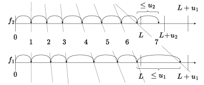
Perhaps the utility of the surrogate process can be better understood through the following frog-race analogy illustrated in Fig. 2. A frog traverses a race track of length jumping from one point to the next. The distance traveled by frog in a single jump is upper bounded by . The jumps are not necessarily IID, but we know that the expected length of each jump is lower bounded by . It is also possible that takes some jumps backwards. With only this information, we want to determine an upper bound on the average number of steps frog takes to reach the end of the track. This could be done using Doob’s optional stopping theorem [22] to compute the upper bound as , the maximum distance traveled from the origin to the last jump divided by the lower bound on average distance of a single jump.
Perhaps this bound can be improved. The final point is located between and and is reached in a single jump from a point between and . If for instance, the frog was restricted to only forward jumps, we could replace by just , but the process actually can take steps backwards. Instead we exploit another property of , which is that maximum step size is not needed to guarantee the lower bound on the average step size.
Suppose now that a surrogate frog participates in the race along but with the following restrictions:
-
1.
and start in the same place and always jump at the same time.
-
2.
is never ahead of , i.e. when jumps forward, jumps at most as far, and when jumps backwards, jumps at least as far.
-
3.
Moreover, the forward distance traveled by frog in a single jump is upper bounded by .
-
4.
Despite its slower progress, the surrogate frog still satisfies the property that the expected length of each jump is lower bounded by .
The average number of steps taken by will be upper bounded by , also by Doob’s optional stopping theorem. Since is never ahead of then crossing the finish line implies that has as well. Thus, is also an upper bound on the average number of jumps required for frog reach across .
The equivalent to the surrogate frog is what we proceed to define in Thm. 2, where the length , , and .
Theorem 2 (Surrogate Process Theorem).
Let the surrogate process be a degraded version of that still satisfies the constraints of Thm. 1. Initialize the surrogate process as and reset to at every , that is at each that the encoder exits a confirmation phase round for message . Define . Suppose that for some , the process also satisfies the following constraints:
| (26) | ||||
| (27) | ||||
| (28) |
Then the total time is not in its confirmation phase is given by , and is bounded by:
| (29) |
Note that for all because from the definition of and constraint (26), Therefore . Also note that after the process terminates at the stopping time , both and are equal to , which makes their difference . Then the communication phase times and are a sum of finitely many non-zero values.
The proof is provided in Sec. V-B
III-C Relaxed Constraints that Achieve a Tighter Bound
The following theorem introduces partitioning constraints that guarantee that the constraints in Thm. 2 are satisfied with a value of for the surrogate process. The new constraints are looser than the original SED constraint, and therefore are satisfied by an encoder that enforces the SED constraint. Using a new analysis we show that this encoder guarantees an achievability bound tighter than the bound (7) obtained in the second step of Yang’s analysis described in Section II. The value is the lowest possible value that satisfies the constraints (26)-(28) of Thm. 2 for a system that enforces the original SED constraint (3). The new achievability applies to an encoder that satisfies the new relaxed constraint as well as one that satisfies the SED constraint.
Theorem 3.
Consider sequential transmission over the BSC with noiseless feedback as described in Sec. I with an encoder that enforces the Small Enough Absolute Difference (SEAD) encoding constraints, equations (30) and (31) bellow:
| (30) | |||
| (31) |
Then, the constraints (19)-(20) in Thm. 1 are satisfied and a process , described in Thm. 2 can be constructed with . The resulting upper bound on is given by:
| (32) |
which is lower than (7) from [2]. Note that meeting the SEAD constraints guarantees that both sets and are non empty. This is because if either set is empty, the the other one is the whole space and the difference in (30) is , which is greater than any posterior in a space with more than one element.
The proof is provided in Sec. V-B
The requirement , is needed to satisfy constraint (19) and guarantees constraint (18). This requirement is also enforced by the SED partitioning constraints in [10] and [2].
The SEAD partitioning constraint is satisfied whenever the SED constraint (3) is. However, the SEAD partitioning constraint allows for constructions of , that do not meet either of the SED constraints in [10] and [2], and is therefore looser. Particularly, SEAD partitioning allows for the case where that often arises in the implementation shown in Sec VII-A. This case is not allowed under either of the SED constraints because they both demand that:
| (33) |
IV Supporting Lemmas and Proof of Theorem 1
This section presents some supporting Lemmas and the full proofs of Thm. 1. Let be the time the transmitted message spends in the communication phase or on an incorrect confirmation phase, that is, for , as defined equation (25). Note that this definition is different from the stopping time used in [2] described in Sec. II. The proof of Thm. 1 consists of bounding and by expressions that derive from the constraints (16)-(20).
Since , the stopping rule described in Sec. II could be expressed by: . To prove Thm. 1, we will instead use the stopping rule introduced by Yang et. al. [2], defined by:
| (34) |
where . This rule models the confirmation phase as a fixed Markov Chain with exactly states. Since , the stopping time under the new rule is larger than or equal to that of the original rule without the ceiling as explained in [2].
IV-A Five Helping Lemmas to Aid the Proof of Thms. 1-3
The expression to bound the expectation expectation is constructed via five inequalities (or equalities) each of which derives from one of the following five Lemmas. The proofs of the Lemmas will be provided in Sec. V-A.
Lemma 1.
Let the total time the transmitted message spends in the communication (or an incorrect confirmation phase) be and let and be as defined in (23) and (24). Define and let
| (35) |
then:
| (36) |
Note that is the time before entering the correct confirmation phase for the first time, that is, the time spent in the communication phase (or an incorrect confirmation phase) before the posterior of the transmitted message ever crosses . If the decoder stops (in error) before ever entering the correct confirmation phase, then is the time until the decoder stops. For , is the time between falling back from the correct confirmation for the time and either stopping (in error) or reentering the correct confirmation phase for the time. Thus, the total time the transmitted message has is also given by . Also note that that if the decoder stops before entering the correct confirmation phase for the time, then for all .
Lemma 3.
Lemma 4.
Let be the decoding threshold and let the decoding rule be (34). Define the fallback probability as the probability that a subsequent round of communication phase occurs, computed at the start of a confirmation phase. Then, this fallback probability is a constant independent of the message , independent of the number of previous confirmation phase rounds , and is given by:
| (40) |
IV-B Proof of Thm. 1 Using Lemmas 1-5:
Proof:
Using Lemmas 1 and 2, the expectation is bounded as follows:
| (43) | ||||
| (44) |
By Lemma (3), expression (44) is equal to the left side of inequality (41), which is bounded by (45) according to Lemma 5:
| (45) |
where is the expected value of the log likelihood ratio of the true message according to the a-priori message distribution, i.e. from the perspective of the receiver before any symbols have been received. Note that is for a uniform a-priori input distribution. Then, equations (43)-(45) yield the following bound on :
| (46) |
A bound on the expectation can be obtained using the Markov Analysis in [2], Section V. F. However, our analysis of already accounts for all time spent in the communication phase, including the additional communication phases that occur after the system falls back from the confirmation phase. Accordingly, we reduce the self loop weight in [2] Sec. V F from to . The resulting bound is given by:
| (47) |
The inequality in (47) is not equality because, in our analysis, the transmission ends if any message , other than the transmitted message , attains . However, in [2] the transmission only terminates when . The upper bound on the expected stopping time is obtained by adding the bounds in equations (46) and (47) and replacing by its definition in equation (34):
| (48) |
Note that and since
, then
which is also used in [2] for a more compact upper bound expression.
∎
V Proof of Lemmas 1-5, Thm. 2, and Thm. 3
Before proceeding to prove Lemmas 1-5, we will introduce a claim that will aid in some of the proofs.
Claim 1.
For the communication scheme described in Sec. II, the following are equivalent:
-
(i)
-
(ii)
or
This claim implies that for constraint (19) to hold, the set containing item , with , must be a singleton.
Proof:
See appendix A ∎
V-A Proof of Lemmas 1-5
Proof:
We begin by defining sets that are used in the proof. First we define , the set of sequences of length where the process has not stopped:
| (49) |
and let .
For each sequence , is the set of time values where message begins an interval with . This includes time zero and all the times where from time to , message transitions from to , i.e. the decoder falls back from confirmation phase to communication phase.
| (50) |
Now we define the set of sequences for which the the following are all true: 1) the decoder has not stopped, 2) the decoder has entered the confirmation phase for message times, and 3) the decoder is not in the confirmation phase for message at time , where the sequence ends.
| (51) |
For , let and let , the concatenation of the strings and . Now we define the set , which is the subset sequences in that have the sequence as a prefix.
| (52) |
As our final definition, let be the set containing only the sequences where the final received symbol is the symbol for which the decoder resumes the communication phase for message for the th time, or the empty string, that is:
| (53) |
Each , sets an initial condition for the communication phase where , so that , that is is of the form defined in (24). By the property of conditional expectation, is given by:
| (54) |
Now we explicitly write this expression as a function of all the possible initial conditions for each of the communication phase rounds , that is, the set :
| (55) | ||||
| (56) | ||||
| (57) |
Now we proceed to write the last expectation (57) using the tail sum formula for expectations in (58) and then as an expectation of the indicator of in (59). Then, since is a random function of , where , given by , (60) follows:
| (58) | ||||
| (59) | ||||
| (60) |
Expanding the expectation in (60) we obtain (61). Since the indicator in (61) is outside and inside, it is omitted in (62), where we have only considered values of that intersect with . Since (62) follows.
| (61) | ||||
| (62) | ||||
| (63) |
The product of the conditional probabilities in (57) and in (63) is given by . Replacing the expectation in (57) by (63) the inner-most sum in (57) becomes (64). The summation in (64) is over for each in , which is equivalent to the sum over and (65) follows:
| (64) | ||||
| (65) |
We can now rewrite (55) by replacing the expectation in (56) by (65) to obtain (66). In (67) the two summations are consolidated into a single sum over union over all of each :
| (66) | ||||
| (67) |
To conclude the proof, note that the union is the set defined in the statement of the Lemma 1. ∎
Proof:
Define the set by:
| (68) |
where does not depend on . Let the set be partitioned into and . Then, we can split the sum in the left side of (69), which is the left side of (38) in Lemma 2, into a sum over , right side of (69), and a sum over the sets , expression (70) as follows:
| (69) | ||||
| (70) |
For s.t. and . Then by constraint (19) and Claim (1), and therefore , (see the proof of Thm. 3, for definition of ). By equation (126) with , this results in for all . Note that means that in this case the SED constraint (3) is satisfied. It suffices to show the bound holds also for (69). The product of conditional probabilities: and in (69) is equal to and can be factored into . Since and does not depend on , then the summation order in (69) can be reversed to obtain:
| (71) |
The probability in (71) is just and using the definition of (72) follows. In (73) is moved inside the expectation, to obtain the form in constraint (20) of Thm. 1:
| (72) | ||||
| (73) | ||||
| (74) |
Constraint (20) dictates that (73) is lower bounded by and (75) follows. Then we multiply by to produce (76). In (77) note that and the product is given . This is used to obtain (77) and then (78):
| (75) | ||||
| (76) | ||||
| (77) | ||||
| (78) |
In both (69) and (70) replacing by provide and upper bound on the original expression. Combining the two upper bounds we recover the Lemma. ∎
Proof:
We start writing, in the left side of (79), the sum in the left side of equation (39) of Lemma 3, using an equivalent form for , which is . This equivalent form was also used in the proof of Lemma 1. Then in (79) we break it into two summations, first over and then over :
| (79) |
The set is a subset of and therefore can be expressed a union of all the intersections over : . We use this new form to rewrite the inner sum in (79) as the left side of (80). Then, we remove the intersections with by using its indicator in the right side of (80):
| (80) |
Recall that from (37). Also recall from (8) that , a random function of . Let , then we expand as:
| (81) |
The product of the probabilities in (80) and (81) is given by . Replacing in (80) using (81) we obtain the left side of (82). The equality in (82) follows by definition of expectation:
| (82) |
We expand using its definition to write (82) as the left side of (83) and use linearity of expectations to the equality (83). The indicator is zero before time and after time , and is one in between. Accordingly, in (84) we adjust the limits of summation and remove the indicator function. Note that the times and are themselves random variables. Lastly, observe that (84) is a telescopic sum that is replaced by the end points in (85):
| (83) | ||||
| (84) | ||||
| (85) |
To conclude the proof, we replace the inner most summation in (79) with (85):
| (86) | ||||
∎
Proof:
The confirmation phase starts at a time of the form defined in (23), at which the transmitted message attains and . Then, like the product martingale in [23], the process , , is a martingale respect to , where:
| (87) |
Note that is a biased random walk, see the Markov Chain in [2], with , where is an R.V. distributed according to:
| (88) |
We verify that as follows:
| (89) |
Let be the time at which decoding either terminates at , or a fall back occurs, when , that is . Then, the process is a two side bounded martingale and:
| (90) | ||||
| (91) |
By Doob’s optional stopping theorem [22], is equal to . Let the fall back probability be , then we can solve for using equations (90) and (91) by setting both right sides equal. In (92) we factor out and cancel . In (93) we collect the terms with factor and in (94) we solve for .
| (92) | ||||
| (93) | ||||
| (94) |
Since is just a function of and , then it is the same constant across all messages and indexes . To complete the proof we use the definition of from equation (5), which is and express in terms of :
| (95) |
∎
Proof:
We start by conditioning the expectation in the left side of equation (41), in Lemma 5, on the events , , and , whose union results in the original conditioning event, , to express the original conditional probability using Bayes rule:
| (96) | |||
Note that is non-negative, thus the last term in the right side of (96) vanishes as . When , then so that . Therefore, the second term in the right side of (96) also vanishes, leaving only the first term conditioned on . Let be the event that message enters confirmation after time , rather than another message ending the process by attaining , that is: . Then, the probability can be expressed as:
| (97) | ||||
Note that the first probability in the right side of (97) is just the fall back probability computed in Lemma 4. The last probability in (97) can be also expressed as a product of conditional probabilities, see (98). In (98) note that event is the event that an -th confirmation phase phase occurs, which implies that a preceding -th communication phase round occurs. Then, and the first factor in the product of probabilities in (98) vanishes:
| (98) |
Combining (97) and (98) we obtain:
| (99) |
We can also bound as follows:
| (100) |
Then, we can recursively bound by using (99) and (100). For , this results in the general bound:
| (101) |
Using (101) we can bound the expectation in the left side of (96) by:
| (102) |
The value of at , when is a constant that can be directly computed for every from the initial distribution. Using (102), we can then bound the second sum in the left side of equation (41) by:
| (103) | ||||
| (104) | ||||
| (105) |
The conditioning event implies events for because if means the process has stopped and no further communication rounds occur. Event also implies that the -th round of communication occurs, and therefore is given by the previous crossing value minus by constraint (19), then:
| (106) | ||||
| (107) |
The inequality in (107) follows from the following inequality:
| (108) |
For the proof of inequality (108) see Appendix D. From (107) it follows that:
| (109) | ||||
| (110) |
In (110) we have factored one inside the expectation. We can now replace (105) by (110) to upper bound (103):
| (111) | ||||
| (112) |
The expectation in (112) combines the two sums in from (111) by subtracting from . The first term is the value of at the communication-phase stopping time . In the second term , the difference is the unique value that can take once the -th confirmation phase round starts at a point . Equation (112) is an important intermediate result in the proof of Thm. 2. This is because when considering the process , the starting value of each communication-phase round is still that of the original process , and therefore the argument of the expectation would change to . For the proof of Lemma 5, we just need to bound (112), so we write the sum in (112) as:
| (113) | ||||
By constraint (17), , and since , then, is bounded by . Thus, the expectation is also bounded by . Then (113) is bounded by:
| (114) |
Finally, the left side of equation (41) in Lemma 5, (the left side of (115)), is upper bounded using the bounds (112) and (114) on the inner sum (109) as follows:
| (115) | ||||
| (116) |
To transition from (115) to (116) we have used the definition of from Lemma 4. The proof of Lemma 5 is complete. ∎
V-B Proof of Theorems 2 and 3
Proof:
Suppose is a process that satisfies the constraints (16)-(20) in Thm. 1 and constraints (26)-(28) of Thm. 2 for some . Because the constraints of Thm. 1 are satisfied, Lemmas 1-5 all hold for the process . To bound we begin by bounding the sum on the right side of Lemma 3, which is (39), but using the new process . Dividing the new bound by produces the desired result. We follow the procedure in the proof of Lemma 5, but replacing by , up to the equation (105). By the definition of we have that and from equation (19) it follows that, for , implies . Then, from equation (105) to (112), we replace by instead. Using equation (112) we have that:
| (117) | ||||
We can replace by using the definition of . We further claim that the constraints of Thm. 2 guarantee that . This is derived from constraint (28): by replacing by . The replacement is possible because , see (94), and by constraint (17). Therefore, the expectation in the last sum can be replaced with for an upper bound to obtain:
| (118) |
Then, the value in equation (118) replaces the inner sum in the left side of (45) to obtain:
| (119) |
The proof is complete. ∎
Proof:
When for some , constraint (31) is the same as the SED constraint (3) and therefore the constraints (19) and (18) are satisfied as shown in [2]. Need to show that constraints (16), (17) and (20) are also satisfied. We start the proof by deriving expressions for to find bounds in terms of the constraints of the theorem. The posterior probabilities are computed according to Bayes’ Rule:
| (120) |
The top conditional probability in equation (120) can be split into . Since the received history fully characterizes the vector of posterior probabilities , and the new construction of and , then the conditioning event sets the value of the encoding function , via its definition: . We can just write the first probability as , which reduces to if and to if . The second probability is just .
The bottom conditional probability can be written as .
By the channel memoryless property, the next output given the input is independent of the past , that is:
.
Since which is given by , we write:
| (121) | ||||
For the encoding function dictates that . Thus , and . Let and and let , so that and . The value of for each can be obtained from equation 121.
Assume first that to obtain the value of .
For the only difference is the sign of the term with . Let , that is if and if and add a coefficient to each for a general expression. Multiply by both terms of the fraction inside the logarithm and expand it to obtain:
| (122) | ||||
| (123) | ||||
| (124) |
Now subtract the term , and add it back as a factor in the logarithm, to recover from . Note that and . And also note that .
The logarithm from (122) is split into , and divides the arguments of the logarithms in (123). Equation (124) follows from applying Jensen’s inequality to the convex function . Then:
| (125) | ||||
| (126) |
By the SEAD constraints, equations (30) and (31) if , then . For the case where , then and . Then the arguments of the logarithms in (126) are both less than for every . This suffices to show that the constraints (20) and (16) are satisfied when for the case that .
It remains to prove that constraints (20) and (16) hold in the case where , or equivalently . Let , and note that since , then:
| (127) |
and and , therefore:
Since this holds for all , then:
| (128) | |||
| (129) |
To satisfy constraint (20) we only need the logarithm term in (129) to be non-negative. This only requires that . Since , then . To satisfy constraint (20) it suffices that , which is equivalent to:
| (130) |
The SEAD constraints, equations (30) and (31), guarantees that . Since , then , which satisfies inequality (130). Then, the SEAD constraints guarantee that constraint (20) is satisfied, and only restricts the (130) is satisfied, and only restricts the absolute difference between and .
To prove that constraint (16) is satisfied, note that equation (30) of the SEAD constraints guarantees that if , then . Starting from equation (124) note that the worst case scenario is when . Using (127) with to go from (131) to (132) we find obtain:
| (131) | ||||
| (132) | ||||
| (133) | ||||
| (134) | ||||
| (135) |
To transition from (134) to (135) we need to show that . For this we find a small constant that makes , the difference between 2 convex functions, also convex. Take second derivatives and and subtract them. The constant is found by noting that .
The SEAD constraints guarantee that both sets, and are non-empty. Then, since the maximum absolute value difference is , constraint (17) is satisfied, see the proof of Claim 1.
For the proof of existence of a process , with , see Appendix B. ∎
VI Extension to Arbitrary Initial Distributions
The proof of Thm. 1 only used the uniform input distribution to assert and replace by in equation (46). In Lemma 5, we have required that . However, even with uniform input distribution this is not the case when . To avoid this requirement, the case where and therefore needs to be accounted for. Also, if , then the probability that an initial fall back occurs is only upper bounded by , which can be inferred from the proof of Lemma 4. Then, to obtain an upper bound on the expected stopping time for an arbitrary input distribution, it suffices to multiply the terms in the proof of Lemma 5, equation (104), by the indicator . Then, the bound on Lemma 5 becomes:
| (136) |
By Thm. 3, we can replace with in (136). Using the definition of from (40) we obtain the bound:
| (137) |
VI-A Generalized Achievability Bound
An upper bound on for a arbitrary initial distribution is then obtained using this bound (137) and the bound on from equation (47) to obtain:
| (138) |
For the special case where , the log likelyhood ratio can be approximated by to obtain a simpler expression of the bound (138):
| (139) |
where is the entropy of the p.d.f. in bits.
VI-B Uniform and Binomial Initial Distribution
Using the bound of equation (138), we can develop a better upper bound on the blocklength for a systematic encoder with uniform input distribution when . It can be shown that the systematic transmissions transform the uniform distribution into a binomial distribution, see [1]. The bound is constructed by adding the systematic transmissions to the bound in (138) applied to the binomial distribution as follows:
| (140) | |||
This bound, which assumes SEAD and systematic transmission, is the tightest achievability bound that we have developed for the model.
VII Algorithm and Implementation
In this section we introduce a systematic posterior matching (SPM) algorithm with partitioning by thresholding of ordered posteriors (TOP), that we call SPM-TOP. The SPM-TOP algorithm guarantees the performance of bound (21) of Thm. 3 because both systematic encoding and partitioning via TOP enforce the SEAD partitioning constraint in equations (30) and (31). The SPM-TOP algorithm also guarantees the performance of the bound (140) because it is a systematic algorithm.
VII-A Partitioning by Thresholding of Ordered Posteriors (TOP)
The TOP rule is a simple method to construct and at any time from the vector of posteriors , which enforces the SEAD partitioning constraint of Thm. 3. The rule requires an ordering of the vector of posteriors such that . TOP builds and by finding a threshold to split into two contiguous segments and . To determine the threshold position, the rule first determines an index such that:
| (141) |
Once is found, the rule must select between two possible alternatives: Either or . In other words, all that remains to decide is whether to place in or in . We select the choice that guarantees that the absolute difference between and is no larger than the posterior of . The threshold is selected from as follows:
| (142) | |||
| (143) |
Note that since , then the posterior of is no larger than that of , and the posterior of is also the value of .
Claim 2.
Proof:
The TOP partitioning rule sets the threshold that separates and exactly before or exactly after item depending on weather case (142) or case (143) occurs. To show that the TOP rule guarantees that the SEAD constraints in Thm. 3 are satisfied note that the threshold lies before item if case (142) occurs. Then, by the first inequality of (141) and by (142):
| (144) | ||||
| (145) |
When case (143) occurs, the threshold is set after item . Then by the second inequality of (141) and by (142):
| (146) | ||||
| (147) |
In either case we have:
| (148) |
By definition, . Scale equation (148) by and subtract , then: . Then, . This concludes the proof. ∎
We have shown that the construction of and can be as simple as finding the threshold item where the c.d.f. induced by the ordered vector of posteriors crosses , then, determining whether the threshold should be before or after item , and finally allocating all items before the threshold to and all items after the threshold to .
VII-B The Systematic Posterior Matching Algorithm
The SPM-TOP algorithm is a low complexity scheme that implements sequential transmission over the BSC with noiseless feedback with a source message sampled from a uniform distribution. The algorithm has the usual communication and confirmation phases and the communication phase starts with systematic transmission. The systematic transmissions of the communication phase are treated as a separate systematic phase, for a total of three phases that we proceed to describe in detail.
VII-C Systematic phase
Let the sampled message be , with bits , that is . For the bits are transmitted and the vector is received. After the -th transmission, both transmitter and receiver initialize a list of groups , where each is a tuple . For each tuple is the count of messages in the group ; is the index of the first message in the group; is the shared Hamming distance between and any message in the group, that is: ; and is the group’s shared posterior. At time , each group has that , , , and . The groups are sorted in order of decreasing probability, equivalent to increasing Hamming weight, since . At the end of the systematic phase, the transmitter finds the index of the group and the index within the group corresponding to the sampled message . The index is given by and the index and is found via algorithm 5. The systematic phase is described by algorithm 1.
VII-D Communication Phase
The communication phase consists of the transmissions after the systematic phase, and while all posteriors are lower than . During communication phase, the transmitter attempts to boost the posterior of the transmitted message, past the threshold , though any other message could cross the threshold instead, due to channel errors.
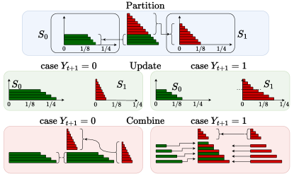
The list of groups initialized in the systematic phase is maintained ordered by decreasing common posterior. The list of groups is partitioned into and before each transmission using rule (141). For this, the group that contains the threshold item is found first, then all groups before are assigned to and all the groups after are assigned to . To assign group the index of item that sets the threshold is determined within group . The TOP rule demands that all items with index be assigned to and all items with index to . For this we split the group into two by creating an new group with the segment of items past that belongs in . However, if the item with index is the last item in , then the entire group belongs in and no splitting is required.
After each transmission , the posterior probabilities of the groups are updated using the received symbol according to equation (120). Each posterior is multiplied by a weight update, computed using equation (121), according to its assignment, or . Then, the lists that comprise and are merged into a single sorted list. The process repeats for the next transmission and the communication phase is interrupted to transition to the confirmation phase when the posterior of a candidate message crosses the threshold. The communication phase might resume if the posterior of message that triggered the confirmation falls below rather than increasing past , and all other posteriors are still below .
Not all groups need to be updated at every transmission. The partitioning method only requires visiting groups . After the symbol is received, we need to combine and into a single list, sorted by decreasing order of posteriors once updated. Figure 3 shows the three operations that are executed during the communication phase: partitioning the list, updating the posteriors of the partitions, and combining the updated partitions into a single sorted list. Note that in both cases, and , either the entirety or a segment of the partition is just appended at the end of the new sorted list. This segment starts at the first group , such that its posterior is smaller than the smallest in . We avoid explicit operations on this segments and only saved the “weight” update factor as another item in the tuple described in at the beginning of this section. Every subsequent item in the list will share this update coefficient and could be updated latter on if it is encountered at either partitioning the list, updating the posteriors or combining the partitions. If this happens, the “weight” update is just “pushed” to the next list item. Since most of the groups belong to this “tail” segment, we expect to perform explicit operations only for a “small” fraction of the groups. This results in a large complexity reduction, which is validated by the simulation data of figure 6.
VII-E Confirmation Phase
The Confirmation Phase is triggered when a candidate attains a posterior . During this phase the transmitter will attempt to boost , the posterior of candidate , past the threshold, if it is the true message . Otherwise it will attempt to drive its posterior below . Clearly, the randomness of the channel could allow the posterior to grow past , even if it is the wrong message, resulting in a decoding error. Alternatively, the right message could still fall back to the communication phase, also due to channel errors. The confirmation phase lasts for as long as the posterior of the message that triggered its start stays between and or equivalently stays between and .
There are no partitioning, update, or combining operations during the confirmation phase. If is the message in the confirmation phase, then the partitioning is just , . A single update is executed if a fallback occurs, letting , where is the index of the confirmation phase round that just ended and is the time at which it started. This is because every negative update that follows a positive update results in every returning to the state it was at time . This is summarized in claim 3 that follows. During the confirmation phase it suffices to check if , in which case the process should terminate, or if , in which case a fall back occurs.
Claim 3 (Confirmation Phase is a Discrete Markov Chain).
Let the partitioning of at time be , , and suppose . If the partitioning at time is also , , the same partitioning of time , and , then for all , , that is .
Proof:
See appendix C ∎
During the confirmation phase we only need to count the difference between boosting updates and attenuating updates. Since the changes in steps with magnitude , then there is a unique number such that and . Starting at time , , since , any event is a boosting update that results in and any event is an attenuating update that results in . A net of boosting updates are needed to reach . Let the difference between boosting and attenuating updates be . The transmission terminates the first time where . However, a fall back occurs if ever reaches before reaching . The value of can be computed as follows: let and let . Suppose the confirmation phase starts at some time , then, if , otherwise . Once is computed, all that remains is to track , where , and return to the communication phase if reaches or terminate the process if reaches .
Theorem 4.
[from [1]] Suppose that and . Then, for the partitioning rule , results in systematic transmission: , and achieves exactly equal partitioning .
Proof:
First note that if , then for each , exactly half of the items in have bit and the other half have bit . The theorem holds for , since the partitioning results in half the messages in each partition and all the messages have the same prior. For note the partitioning only considers the first bits of each message . Thus, all item that share a prefix sequence have shared the same partition at times , and therefore share the same posterior. There are exactly such difference posteriors. Also, exactly half of the items that share the sequence have bit and are assigned to at time and the other half have bit and are assigned to at time . Then, and will each hold half the items in each posterior group at each next time for , and therefore equal partitioning holds also at times . ∎
VII-F Complexity of the SPM-TOP Algorithm
The memory complexity of the SPM-TOP algorithm is of order because we use a triangular array of all combinations of the form . The algorithm itself stores a list of groups that grow linearly with , since the list size is bounded by the decoding time .
The time complexity of the SPM-TOP algorithm is of order . To obtain this result note that the total number of items that the system tracks is bounded by the transmission index . At each transmission , partitioning, update and combine operations require visiting every item at most once. Furthermore, because of the complexity reduction described in Sec. VII-D, the system executes operations for only a fraction of all the items that are stored. The time complexity at each transmission is then of order , with a small constant coefficient. The number of transmissions required is approximately as the scheme approaches capacity. A linear number of transmissions, each of which requires a linear number of operations, results in an overall quadratic complexity, that is, order , for fixed channel capacity .
The systematic transmissions only require storing the bits, and in the confirmation phase we just add each symbol to the running sum. The complexity of this phase is then of order . Therefore, the complexity of is only for the communication phase.
VIII SPM-TOP simulation results
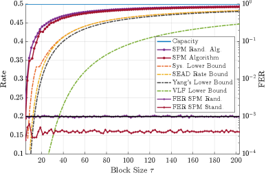
We validate the theoretical achievability bounds in Sec. III and Sec. VI via simulations of the SPM-TOP algorithm. Figure 4 shows Simulated rate vs. blocklength performance curves of the SPM-TOP algorithm and the corresponding frame error rate (FER). The plots show simulated rate curves for the standard SPM-TOP algorithm and a randomized version, as well as their associated error rate. The rate for the standard SPM-TOP algorithm is shown with the red curve with dots at the top and the corresponding FER is the red, jagged curve at the bottom. The standard SPM-TOP algorithm stops when a message attains . Note that the FER is well below the threshold . The randomized version of the SPM-TOP algorithm, implements a stopping rule that randomly alternates between the standard rule, which is stopping when a message attains , and stopping when a message attains , which requires one less correctly received transmission. The simulated rate of the randomized SPM-TOP version is the purple curve above the standard version. This randomized version aims to obtain a higher rate by forcing the FER to be close to the threshold rather than upper bounded bounded by . Note that the corresponding FER, the horizontal purple curve with dots, is very close to the threshold , but not necessarily bounded above by the threshold. The simulation consisted of trials for each value of and for a decoding threshold and a channel with capacity . The simulated rate curves attain an average rate that approaches capacity rapidly and stay above all these theoretical bounds, also shown in Figure 4 that we describe next.
The two rate lower bounds introduced in this paper are shown in Figure 4 for the same channel, capacity and threshold , used in the simulations. The highest lower bound is labeled Sys. Lower Bound, and is the bound developed in Sec. VI-B for a system that uses a systematic phase to turn a uniform initial distribution into a binomial distribution and then enforces the SEAD constraints. The next highest bound is labeled SEAD Rate Bound and is the lower bound (32) introduced in Thm. 3 for a system that enforces the SEAD constraints. This bound is a slight improvement from the SED lower bound by Yang et al. [2] that we show for comparison and is labeled Yang’s Lower Bound. Also for comparison, we show Polyanskiy’s VLF lower bound developed for a stop feedback system. Since a stop feedback system is less capable than a full feedback system, we expect that the lower bound for full feedback system approaches capacity faster than the VLF bound, which is what the previous bounds achieve.
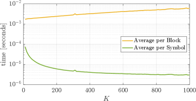
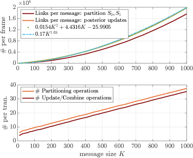
The empirical time complexity results of the SPM-TOP algorithm simulations vs. message size is shown in Figures 5 and Figure 6. All simulations were performed on a 2019 MacBook Pro laptop with a GHz, -core processor and GB of RAM, and with transmitter and receiver operating alternatively on the same processor. First we show in Figure 5 the average time, in milliseconds, taken per message, yellow line, and per transmitted symbol, green line. The average time per symbol drops very fast as the message size grows from to and then slowly stabilizes. This drop could be explained by the initialization time needed for each new message. However, the computer temperature and other processes managed by the computer’s OS could also play a role in time measurements. For a more accurate characterization of the complexity’s evolution as a function of message size , we count the number of operations executed during the transmission of each symbol and each message, which are probability checks for partitioning before transmitting a symbol and probability updates after the transmission of a symbol.
The average number of probability checks and probability update operations per message vs message size are shown in the top of Figure 6. To compare the data with a quadratic line, we fitted the parabola to the update-merge simulated data. Also for reference, the blue line shows the function to highlight that the complexity per message is below quadratic in the region of interest. The average number of probability checks and probability update operations per transmitted symbol are shown in the bottom of Figure 6. The number of operations per symbol falls well below , even when the number of probabilities that the system tracks is larger than . This number is at and only increases with . Note that for both averages are below . These results show that complexity of the SPM-TOP algorithm allows for fast execution time and validate the theory that the complexity order as a function of is linear for each transmission and quadratic for the whole message.
IX Conclusion
Naghshvar et al. [10] established the “small enough difference” (SED) rule for posterior matching partitioning and used martingale theory to study asymptotic behavior and also showed how to develop a non-asymptotic lower bound on achievable rate. Yang et al. [2] significantly improved the non-asymptotic achievable rate bound using martingale theory for the communication phase and a Markov model for the confirmation phase, still maintaining the SED rule. However, partitioning algorithms that enforce the SED rule require a complex process of swapping messages back and forth between the two message sets and and updating the posteriors.
To reduce complexity, this paper replaces SED with the small enough absolute difference (SEAD) partitioning constraints. The SEAD constraints are more relaxed than SED, and they admit the TOP partitioning rule. In this way, SEAD allows a low complexity approach that organizes messages according to their type, i.e. their Hamming distance from the received word, orders messages according to their posterior, and partitions the messages with a simple threshold without requiring any swaps.
The main analytical results show that the SEAD constraints suffice to achieve at least the same lower bound that Yang et al. [2] showed to be achievable by SED. Moreover, the new SEAD analysis establishes achievable rate bounds higher than those found by Yang et al. [2]. The analysis does not use martingale theory for the communication phase and applies a surrogate channel technique to tighten the results. An initial systematic transmission further increases the achievable rate bound.
The simplified encoder associated with SEAD has a complexity below order and allows simulations for message sizes of at least 1000 bits. These simulations reveal actual achievable rates that are enough above our new achievable-rate bounds that further analytical investigation to obtain even tighter achievable-rate bounds is warranted. From a practical perspective, the simulation results themselves provide new lower bounds on the achievable rates possible for the BSC with full feedback. For example, with an average block size of 200.97 bits corresponding to message bits, simulation results for a target codeword error rate of show a rate of for the channel with capacity 0.5, i.e. % of capacity.
X Acknowledgements
The authors would like to thank Hengjie Yang and Minghao Pan for their help with this manuscript.
Appendix A Proof of claim 1
Proof that is equivalent to ( or ). First let’s prove the converse, if the set containing is not singleton, then constraint (19) does not hold. Without loss of generality, assume and suppose s.t. . Since , then, . By equation (123), when , then:
| (149) | ||||
| (150) |
Note from equation (149) that decreases with , therefore, replacing with a lower bound gives an upper bound of difference (149). For a lower bound, note that , and that setting in (149), results in . In the case where , or , by equation (123), the difference is:
| (151) | ||||
| (152) | ||||
| (153) | ||||
| (154) |
To prove that if the set containing is singleton, then , note that . The inequalities, therefore, become equalities and equations (149) and (151) become and respectively.
Appendix B Proof of existence of in Thm. 2
The proof that a process like the one described in Thm. 2 exists, consists of constructing one such process. Define the process by if and define , where, to enforce constraints (16) and (20), if , the update is defined by (162), and when , in which case , to enforce constraints (11) and (19) the update is given by .
Denote the transmitted symbol by , and the received symbol by and let . The symbol could either be or . Also, we could have or . These cases combine to possible events. Define , and note that can be derived from equation (123) as follows:
| (155) |
where , , and are given by:
| (156) | ||||
| (157) | ||||
| (158) | ||||
| (159) |
Let and be defined by:
| (160) | ||||
| (161) |
then, define the update by:
| (162) |
Need to show that the constraints (20)-(19) of Thm. 1, and constraints (26) and (28) are satisfied. When , since is defined in the same manner as , then constraints (18) and (19) are satisfied.
The proof that satisfies constraints (20), (16) and (26) is split into the case where and the case where .
B-A Case .
It suffices to show that for all and for all , if , then , Since (constraint (16)), and any weighted average would add up to (constraint (20)).
When , then , and therefore, since . The expectation can be computed from (123), where depends on whether or . The expectation is given by either (163) or (164) respectively:
| (163) | |||
| (164) |
This proofs constraints (20) and (16) satisfied. To proof that constraint (26) is satisfied, need to show that . If suffices to compare the cases where , when . It suffices to compare the terms in which the pairs differ, that is, that and . For this comparison, express and as positive logarithms as follows:
| (165) | ||||
| (166) | ||||
| (167) | ||||
| (168) |
Since , then, we only need to show that the arguments of the logarithm in (165) is greater than that of (166), and similarly for (167) and (168). All arguments share the term , then only inequalities (169) and (170) to hold:
| (169) | ||||
| (170) |
The numerators on both inequalities are the same, and positive, since that and if then and for all cases regardless. Both denominators on the left hand side are smaller than those in the right side, by exactly the numerators, and therefore, the inequalities hold.
B-B Case .
Next we show that constraints (20), (16) and (26) are satisfied when . In the case where , then is still by equation (167). However, whenever , the term is added to . To show that constraint (20) holds, recall from (126) that:
| (171) | ||||
| (172) | ||||
| (173) |
To obtain , replace by in equation (173), and let . Then and , and replace to obtain:
| (174) | ||||
| (175) | ||||
| (176) | ||||
| (177) | ||||
| (178) |
To show that , (constraint (16)), note that is either unchanged from , or the same as when and therefore, it holds for . For , note from the first term of equation (174), that . Since , then the expectation is either or greater.
Need to show, (constraint (26)). It suffices to show that and . Again, since is either or the same as when , we only need to show that . It suffices to show that for a positive scalar :
| (179) |
When , then . We have that:
| (180) |
Recall from equation (129) that:
| (181) |
and let , then, the scaled difference between left and right terms in (179) is given by:
| (182) | ||||
| (183) | ||||
| (184) | ||||
| (185) |
Equation (182) follows from (181). In (183), Jensen’s inequality is used, where:
. In (184) note that . Finally .
We conclude that , and therefore .
B-C Proof of constraint (28)
Finally need to show that constraint (28) is satisfied, that is: . We have shown that the update allows the process to meet constraints (16)-(19) of Thm. (1) and constraints (26) and (26). Note that by the definition of in Thm. 2 it is possible that the process restarts when falls from confirmation, at a time , without ever attaining . We could construct a third process that preserves all the properties of , and with if . The process could be initialized by and then letting with step size defined by: . The inner minimum guarantees that reaches if does, and the outer maximum guarantees that the step size is at least that of . Then the processes and cross at the same time, and share the same values when , that is:
| (186) | ||||||
| (187) |
Using the process and equation (187), the expression in constraint (28) becomes:
| (188) |
In the case where , we have that
and , then:
| (189) | ||||
| (190) | ||||
| (191) |
The first inequality in (191) follows since and the second inequality holds because:
| (192) |
For the case where we solve a constraint maximization of expression (188), where the constraint is (or ). For simplicity we subtract the constant from (188).
Let be arbitrary and let , and . Using the definitions of and in (155), (162) and (160)-(161), we explicitly find expressions for in terms of , , and .
When or the expression is given by:
| (193) | |||
and when or it is given by:
| (194) | |||
B-D Maximizing (193)
The maximum of (193) happens when , since the term with the indicator function is non-negative. Since , then , and we proceed to solve:
| (195) | |||
| (196) |
where is defined by:
| (197) | |||
First we show that is increasing in , by showing . Note that and
| (198) |
Factor out the positive constant , to obtain:
| (199) | |||
| (200) |
It suffices to show that the top of equation (200) is non-negative. Since it decreases when then:
| (201) | ||||
| (202) | ||||
| (203) | ||||
| (204) |
In equation (204) we have used and . Since then is increasing in and we can replace by for an upper bound. Since , then is given by:
| (205) | ||||
| (206) | ||||
| (207) |
To complete the proof, it suffices to show that the last expression decreases in :
| (208) | ||||
| (209) | ||||
| (210) | ||||
| (211) |
Since is decreasing, then the maximum of equation (193) is , at .
B-E Maximizing (194)
The expression (194) is given by where is defined by:
| (212) | ||||
We proceed to solve:
| maximize | (213) | |||
| subject to | (214) |
Combining the last two terms we obtain:
| (215) |
The first term increases with , and the second one decreases as the quotient increases in absolute value. For , it is possible to have , leaving only (215). However, for , the quotient is positive because . The smallest value of the quotient is then with square . Let be defined in equation (216), then the maximum of is bounded by the maximum of , where:
| (216) | ||||
To determine the max, we find the behavior of by taking the first derivative:
| (217) |
Then, scale by the positive term to obtain:
| (218) | ||||
| (219) | ||||
| (220) | ||||
| (221) | ||||
| (222) |
To show that in it suffices to show that the top of equation (222) is positive:
| (223) | ||||
| (224) | ||||
| (225) | ||||
| (226) | ||||
| (227) |
When , then and the second term is non-negative and therefore the derivative is positive. When we have , , then:
therefore, is increasing in and the maximum is at where . The maximum is given by:
| (228) |
Then the maximum of is zero. Since the maximum of both equations, (193) and (194) are zero, we conclude that .
Finally, we prove the last claim that is the smallest value for a system that enforces the SED constraint. It suffices to note that the surrogate process described in [2], Sec. V E is a strict martingale. A process with a lower value would not comply with constraint (9) and therefore would also fail to meet constraint (20).
Appendix C Proof: Confirmation Phase State Space 3
Proof:
Suppose that for times and the partitioning is fixed at and . Suppose also that , and . Need to show that we have that . Using the update formula (121), at time we have that for :
| (229) | ||||
| (230) |
At time , since , equation (121) for results in:
| (231) | ||||
| (232) |
And for equation (121) results in:
| (233) | ||||
| (234) |
Then for all each posterior at time is given by: . The same equalities hold when and , where the only difference is that and are interchanged. By induction, we have that for , if for every the partitions are fixed at and , and . ∎
Appendix D Proof of Inequality (108), Sec. III
Proof:
Need to show that the following inequality holds:
| (235) |
Recall that is the event that message enters confirmation after time , rather than another message ending the process by attaining . This event is defined by . Using Bayes rule, the expectation can be expanded as a sum of expectations conditioned on events that are defined in terms of , and , and whose union is the full event space to leave only the original conditioning . These events are , , and . Note that and therefore the third event vanishes. The expansion is given by:
| (236) | ||||
| (237) | ||||
| (238) |
Since , we can omit the conditioning on and when accompanied by . By the independence of the confirmation phase from the crossing value derived from the fix state count of the Markov Chain we have that:
| (239) |
Therefore, we can replace the expectation in (237) by the one in (236) and then add the probabilities in (236) and (237) to obtain . Note that , thus the conditioning on is redundant with . Then the expectation in the left of (236) is also given by:
| (240) | ||||
| (241) |
The event implies that the process decodes in error at the th communication phase round, which results in . Therefore, we have that , This makes the left side of (240) an average of the positive quantity in the right of (240) and the negative quantity in (241). Then:
| (242) | ||||
| (243) |
The last inequality (243) follows because the expectation is positive and is multiplied by a probability, , in (242). ∎
References
- [1] A. Antonini, H. Yang, and R. D. Wesel, “Low complexity algorithms for transmission of short blocks over the bsc with full feedback,” in 2020 IEEE International Symposium on Information Theory (ISIT), 2020, pp. 2173–2178.
- [2] H. Yang, M. Pan, A. Antonini, and R. D. Wesel, “Sequential transmission over binary asymmetric channels with feedback,” IEEE Tran. Inf. Theory, 2021. [Online]. Available: https://arxiv.org/abs/2111.15042
- [3] C. Shannon, “The zero error capacity of a noisy channel,” IRE Trans. Inf. Theory, vol. 2, no. 3, pp. 8–19, September 1956.
- [4] M. V. Burnashev, “Data transmission over a discrete channel with feedback. random transmission time,” Problemy Peredachi Inf., vol. 12, no. 4, pp. 10–30, 1976.
- [5] M. Horstein, “Sequential transmission using noiseless feedback,” IEEE Trans. Inf. Theory, vol. 9, no. 3, pp. 136–143, July 1963.
- [6] O. Shayevitz and M. Feder, “Optimal feedback communication via posterior matching,” IEEE Trans. Inf. Theory, vol. 57, no. 3, pp. 1186–1222, March 2011.
- [7] S. K. Gorantla and T. P. Coleman, “A stochastic control approach to coding with feedback over degraded broadcast channels,” in 49th IEEE Conference on Decision and Control (CDC), 2010, pp. 1516–1521.
- [8] C. T. Li and A. E. Gamal, “An efficient feedback coding scheme with low error probability for discrete memoryless channels,” IEEE Trans. Inf. Theory, vol. 61, no. 6, pp. 2953–2963, June 2015.
- [9] O. Shayevitz and M. Feder, “A simple proof for the optimality of randomized posterior matching,” IEEE Trans. Inf. Theory, vol. 62, no. 6, pp. 3410–3418, June 2016.
- [10] M. Naghshvar, T. Javidi, and M. Wigger, “Extrinsic Jensen–Shannon divergence: Applications to variable-length coding,” IEEE Trans. Inf. Theory, vol. 61, no. 4, pp. 2148–2164, April 2015.
- [11] J. H. Bae and A. Anastasopoulos, “A posterior matching scheme for finite-state channels with feedback,” in 2010 IEEE Int. Symp. Inf. Theory, 2010, pp. 2338–2342.
- [12] V. Kostina, Y. Polyanskiy, and S. Verd, “Joint source-channel coding with feedback,” IEEE Trans. on Inf. Theory, vol. 63, no. 6, pp. 3502–3515, 2017.
- [13] S. Kim, R. Ma, D. Mesa, and T. P. Coleman, “Efficient bayesian inference methods via convex optimization and optimal transport,” in 2013 IEEE Int. Symp. on Inf. Theory, 2013, pp. 2259–2263.
- [14] O. Sabag, H. H. Permuter, and N. Kashyap, “Feedback capacity and coding for the bibo channel with a no-repeated-ones input constraint,” IEEE Tran. Inf. Theory, vol. 64, no. 7, pp. 4940–4961, 2018.
- [15] L. V. Truong, “Posterior matching scheme for gaussian multiple access channel with feedback,” in 2014 IEEE Information Theory Workshop (ITW 2014), 2014, pp. 476–480.
- [16] A. Anastasopoulos, “A sequential transmission scheme for unifilar finite-state channels with feedback based on posterior matching,” in 2012 IEEE Int. Symp. Inf. Theory, 2012, pp. 2914–2918.
- [17] J. Schalkwijk, “A class of simple and optimal strategies for block coding on the binary symmetric channel with noiseless feedback,” IEEE Trans. Inf. Theory, vol. 17, no. 3, pp. 283–287, May 1971.
- [18] J. Schalkwijk and K. Post, “On the error probability for a class of binary recursive feedback strategies,” IEEE Trans. Inf. Theory, vol. 19, no. 4, pp. 498–511, July 1973.
- [19] A. Tchamkerten and E. Telatar, “A feedback strategy for binary symmetric channels,” in Proc. IEEE Int. Symp. Inf. Theory, June 2002, pp. 362–362.
- [20] A. Tchamkerten and I. E. Telatar, “Variable length coding over an unknown channel,” IEEE Trans. Inf. Theory, vol. 52, no. 5, pp. 2126–2145, May 2006.
- [21] M. Naghshvar, M. Wigger, and T. Javidi, “Optimal reliability over a class of binary-input channels with feedback,” in 2012 IEEE Inf. Theory Workshop, Sep. 2012, pp. 391–395.
- [22] R. Durrett, Probability : theory and examples / Chapter 4.8, Optional Stopping Theorems, 5th ed., ser. Cambridge series in statistical and probabilistic mathematics ; 49. Cambridge ;: Cambridge University Press, 2019.
- [23] ——, Probability : theory and examples / Chapter 4.2, Exponential Martingale, 5th ed., ser. Cambridge series in statistical and probabilistic mathematics ; 49. Cambridge ;: Cambridge University Press, 2019.