ACLS: Adaptive and Conditional Label Smoothing for Network Calibration
Abstract
We address the problem of network calibration adjusting miscalibrated confidences of deep neural networks. Many approaches to network calibration adopt a regularization-based method that exploits a regularization term to smooth the miscalibrated confidences. Although these approaches have shown the effectiveness on calibrating the networks, there is still a lack of understanding on the underlying principles of regularization in terms of network calibration. We present in this paper an in-depth analysis of existing regularization-based methods, providing a better understanding on how they affect to network calibration. Specifically, we have observed that 1) the regularization-based methods can be interpreted as variants of label smoothing, and 2) they do not always behave desirably. Based on the analysis, we introduce a novel loss function, dubbed ACLS, that unifies the merits of existing regularization methods, while avoiding the limitations. We show extensive experimental results for image classification and semantic segmentation on standard benchmarks, including CIFAR10, Tiny-ImageNet, ImageNet, and PASCAL VOC, demonstrating the effectiveness of our loss function.
1 Introduction
Humans have an ability to make well-calibrated decisions, such that confidence levels of decisions reflect likelihoods of underlying events accurately. On the contrary, deep neural networks (DNNs) often struggle to achieve such levels of calibration, which is problematic particularly in applications involving high levels of uncertainty and reasoning, including autonomous driving [9, 31, 13] and medical diagnosis [14, 23, 1]. For example, supervised approaches to image classification typically exploit one-hot encoded labels and a softmax cross-entropy loss [10, 26, 3, 19] to train the networks. The loss encourages minimizing the entropy of network outputs, i.e., preferring the Dirac delta distribution with a peak at the one-hot label, which causes overconfident predictions, while overly penalizing uncertainty in the predictions [19].
Recently, a variety of confidence calibration methods have been introduced to address this problem [26, 3, 19, 12, 25, 10, 8, 27, 6, 22], which can broadly be divided into two categories: Post-hoc methods and regularization-based methods. Post-hoc approaches to network calibration adjust the predictions of a pre-trained model at test time, typically using additional trainable parameters [30, 10, 6]. For example, a temperature scaling technique [30] multiplies logits by a temperature parameter, resulting in a softened distribution of predictions that can help mitigate the overconfidence problem. While post-hoc approaches are effective and computationally cheap, they mainly have two limitations. First, they require a held-out dataset to tune the additional parameters [12, 26]. Second, post-hoc approaches assume that training and test samples are drawn from the same distribution [19], which limits performance under distribution shifts between training and test datasets [16, 26, 12]. Regularization approaches integrate calibration techniques into the training process, e.g., in a form of objective functions [19, 12, 25, 3, 26]. These methods regularize network outputs implicitly [26, 27] or explicitly [19, 12, 25, 3] by penalizing overconfident or underconfident predictions, encouraging the distribution of predictions to be uniform. While regularization approaches have shown the effectiveness, the influence of regularization terms on network calibration remains unclear, and only a limited number of studies have explored to delve deeper into these approaches. For instance, the works of [27, 19] have demonstrated that the label smoothing technique [32] is also effective for network calibration. In addition, the focal loss [18], which was initially developed for object detection, has been proven to raise the entropy of network predictions, performing regularization implicitly [26, 19].
We present in this paper a theoretical and empirical analysis of various regularization-based methods, including LS [32], FLSD [26], CPC [3], MDCA [12], MbLS [19], and CRL [25], to better understand the underlying principles of these approaches. Our analysis on the gradients of objective functions for the regularization-based methods reveals that 1) these methods can be viewed as variants of the label smoothing technique [32], and differ only in how they determine the degree of label smoothing, and 2) they do not always behave as expected, and often produce undesired results in terms of network calibration. We further categorize the regularization-based methods into three groups based on the type of label smoothing: Adaptive regularization (AR) [3, 12], conditional regularization (CR) [19], and a combination of them [25]. AR adjusts the strength of regularization for (one-hot encoded) training labels adaptively based on output probabilities of a network across classes, which is more beneficial for network calibration than the vanilla label smoothing technique (CPC [3], MDCA [12] vs. LS [32] in Table 1). Ideally, the label of a true class should decrease in accordance with the degree of increase in a corresponding output probability, whereas the labels of false classes should increase proportionally with the degree of decrement in each output probability. However, our observation suggests that the regularization-based methods using AR [3, 12] do not consistently behave as in the ideal scenario. Specifically, when the output probability is exceedingly high, the label of a true class rather decreases slightly. CR modifies training labels selectively based on a specific criterion, e.g., using margin-based penalties [19]. Since output probabilities of a network are not always miscalibrated, CR performs regularization on the miscalibrated ones only, thus showing better calibration capability than the label smoothing technique (MbLS [19] vs. LS [32] in Table 1). However, MbLS [19] using CR is not likely to regularize the training label of a true class, which leads to the overconfidence problem. A hybrid method, e.g., CRL [25], takes advantages of AR and CR, but it would inherit the limitations of both approaches. We will provide a more detailed analysis in Sec. 3.2.
Based on the gradient analysis for the regularization-based approaches, we introduce a novel loss function, dubbed ACLS, for network calibration. ACLS combines the strengths of AR and CR, while mitigating the drawbacks of the regularization-based methods [3, 12, 19, 25, 18, 26, 32], providing better calibration results (Table 1). On the one hand, it determines the degree of label smoothing adaptively for each class, while avoiding the undesirable aspects observed in the regularization-based methods using AR [3, 12]. Specifically, ACLS regularizes the labels of true object classes more strongly, as corresponding output probabilities increase, and vice versa for other classes. On the other hand, it exploits a predefined margin to determine whether to adjust training labels, similar to the regularization method using CR [19], but also modifies the label of a true class to smooth a corresponding probability, preventing the overconfidence problem. Experimental results on standard benchmarks [5, 15, 17, 7] demonstrate that networks trained with ACLS outperform the state of the art in terms of expected calibration error (ECE) and adaptive ECE (AECE). Our main contributions can be summarized as follows:
-
Based on the analysis, we present a new loss function, ACLS, that retains the advantages of AR and CR, while overcoming the negative effects of existing calibration methods.
2 Related work
Post-hoc calibration.
A pioneer work of [10] proposes to calibrate predictions of a pre-trained DNN for image classification at test time, using a temperature scaling technique [30]. It regularizes the distribution of the predictions in a way of minimizing negative log-likelihood or ECE using a temperature parameter. ETS [36] aggregates various temperature scaling techniques to improve the calibration performance. Instead of using ensemble, the work of [33] proposes to estimate temperatures for individual samples adaptively. A recent work of [6] extends the temperature scaling technique for dense prediction tasks (e.g., semantic segmentation). Although these calibration methods are straightforward and effective, they reduce all output probabilities of a network, without considering confidence levels of individual predictions. It is thus highly likely that well-calibrated predictions could also be altered, which rather degrades the overall calibration performance [16, 26, 12]. Moreover, tuning hyperparameters (e.g., the temperature) requires additional held-out datasets, which makes it challenging to deploy post-hoc calibration methods in practical settings [12].
Regularization-based calibration.
Many attempts to calibrating neural networks have been made using regularization-based approaches. The seminal work of [29] suppresses overconfident predictions, while maximizing the entropy of network outputs. FLSD [26] proposes to exploit the focal loss (FL) [18] for network calibration. In particular, it adjusts a focusing parameter adaptively to concentrate more on hard examples, alleviating the overconfidence problem. However, the FL ignores easy training samples, which causes the underconfidence problem [8]. FLSD also uses heuristics to determine the focusing parameter which is not optimal for all samples. AdaFocal [8] addresses these problems by setting the focusing parameter for each sample based on a calibration metric and exploiting an inverse focal loss [34] to put more focus on easy samples. MbLS [19] proposes to exploit margin-based penalties to selectively regularize miscalibrated predictions. Recently, the works of [3, 12, 25] present new regularization terms for network calibration. Specifically, CRL [25] formulates network calibration as an ordinal ranking problem [4], and determines whether to penalize predictions of a network in order to obtain better confidence estimates. CPC [3] decouples multi-class predictions into multiple binary ones, and calibrates pairs of binary predictions, augmenting the number of supervisory signals, compared to the softmax cross-entropy loss. MDCA [12] introduces a differentiable version of static calibration error (SCE) [28], enabling optimizing a network directly in terms of SCE.
Although regularization-based methods have proven effective in calibrating networks, there have been limited efforts to explore the underlying principles behind these approaches. The work of [26] offers both theoretical and empirical justifications of using the focal loss [18] for calibrating networks. In particular, it shows that the focal loss minimizes implicitly the Kullback-Leibler (KL) divergence between a uniform distribution and softmax predictions, regularizing the distribution of network predictions. The label smoothing technique [32], which improves the discriminative ability of DNNs, has been demonstrated to be effective for network calibration [27, 19]. Similar to the finding in [26], the work of [19] highlights that a cross-entropy loss with the label smoothing augments the KL divergence between a uniform distribution and softmax predictions. It also demonstrates that the focal loss can be regarded as a form of label smoothing, which effectively alleviates the overconfidence problem. Taking one step further, we show that existing regularization-based methods, including FLSD [26], CPC [3], MDCA [12], MbLS [19], and CRL [25], can be considered as variants of the label smoothing technique. We also provide a comprehensive analysis on gradients of objective functions for these methods, and show that the objective functions have detrimental effects on network calibration.
3 Method
In this section, we first describe preliminaries on network calibration (Sec. 3.1). We then provide an in-depth analysis of regularization-based methods [3, 12, 19, 25, 18, 26] in terms of gradients of objective functions (Sec. 3.2), and introduce our loss function, ACLS, for network calibration (Sec. 3.3).
3.1 Network calibration
Given an input and a corresponding ground-truth label (class) , DNNs output a logit vector , where is the number of classes. To train DNNs, a softmax CE loss is generally used as follows:
| (1) |
where represents a softmax output of the network, and indicates a target distribution (i.e., a distribution of one-hot encoded labels). We denote by and elements of and for the class , respectively. We define the softmax output for the class as follows:
| (2) |
where we denote by the logit value of for the class . Formally, we compute gradients of w.r.t the logit for the class as follows:
| (3) |
The CE loss encourages minimizing the discrepancies between probability distributions of and , learning discriminative feature representations. To this end, the probability for the true class should be one, the same as . Accordingly, the CE loss tries to raise the corresponding logit (or equivalently the probability ), although the probability could not reach to the value of one exactly [32], resulting in the overconfidence problem [10, 26, 3, 19, 32].
Label smoothing.
To address the overconfidence problem, label smoothing [32] modifies the target distribution as follows:
| (4) |
where is a hyperparameter for controlling the degree of smoothing. It lowers the initial target probability for the true class , while raising the probabilities for others. For better understanding its behavior, we compute the gradients of the objective function for label smoothing w.r.t the logit , which is the same as the CE loss in Eq. (1) but with the target distribution of , as follows:
| (5) |
where and . In contrast to the CE, the probability of for the true class would be the same as that of . The logit value will thus not be raised continually, mitigating the overconfidence problem. Note that the gradients for label smoothing in Eq. (5) reduce to those for CE in Eq. (3) with being zero. In the following, we will show that existing regularization-based methods can be considered as variants of label smoothing.
3.2 Gradient analysis
Regularization approaches to network calibration generally exploit a regularization term along with a fidelity being the CE loss to alleviate the miscalibration problem. Although they have proven effective in network calibration, there is a lack of theoretical understandings on how the regularization term affects on the calibration. To better understand the effects on calibration, we compute gradients of objective functions for existing regularization-based methods (Table 2).
Concretely, we can represent the loss functions of calibration methods [3, 12, 19, 25, 18, 26] as follows:
| (6) |
where is a regularization term. We compute the gradient of Eq. (6) w.r.t the logit value for the class :
| (7) |
which can be reformulated as follows:
| (8) |
where we denote by a network prediction. is a smoothing function that determines the degree of smoothing, and is an indicator function deciding whether to apply smoothing or not. Note that the network calibration methods are designed to lower the largest output probability across the classes, where the overconfidence problem is likely to occur. The gradients in Eq. (8) are thus split based on the network prediction , in contrast to label smoothing [32] using the ground-truth label in Eq. (5). We can see that 1) the gradients of existing regularization-based methods in Eq. (8) generalize those for label smoothing in Eq. (5) if the prediction is correct (i.e., ), and 2) each method differs in how smoothing and indicator functions are defined (Table 2), suggesting that the regularization-based methods can be regarded as a form of label smoothing. We provide detailed derivations and explanations of smoothing and indicator functions for each method in the supplementary material.
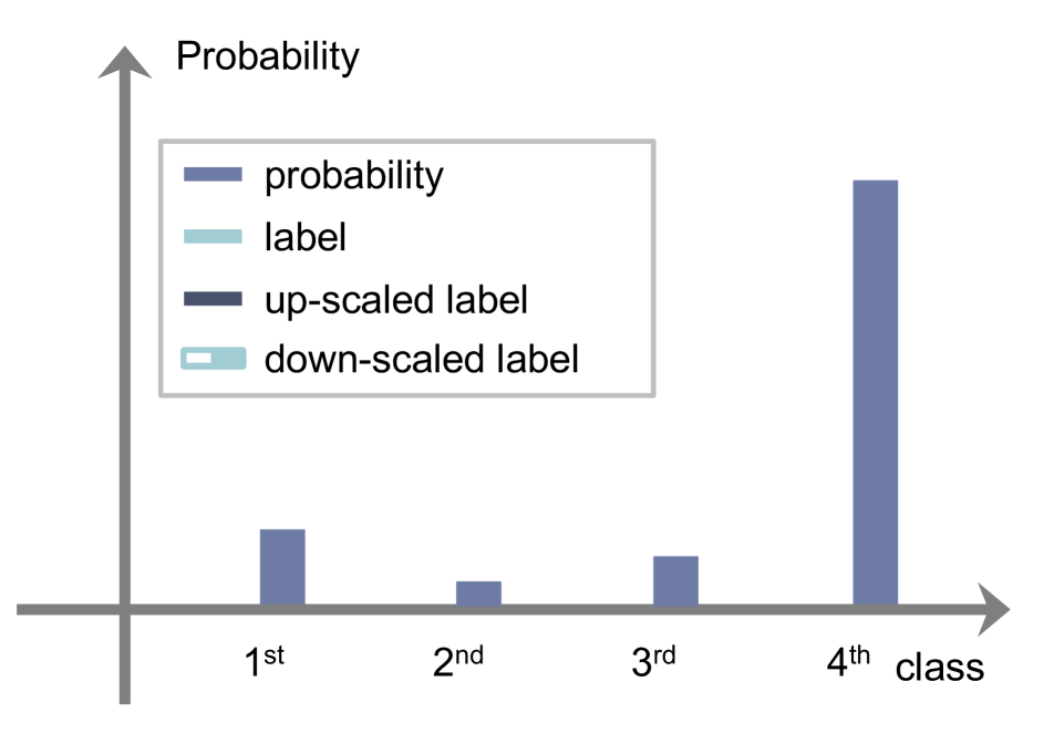
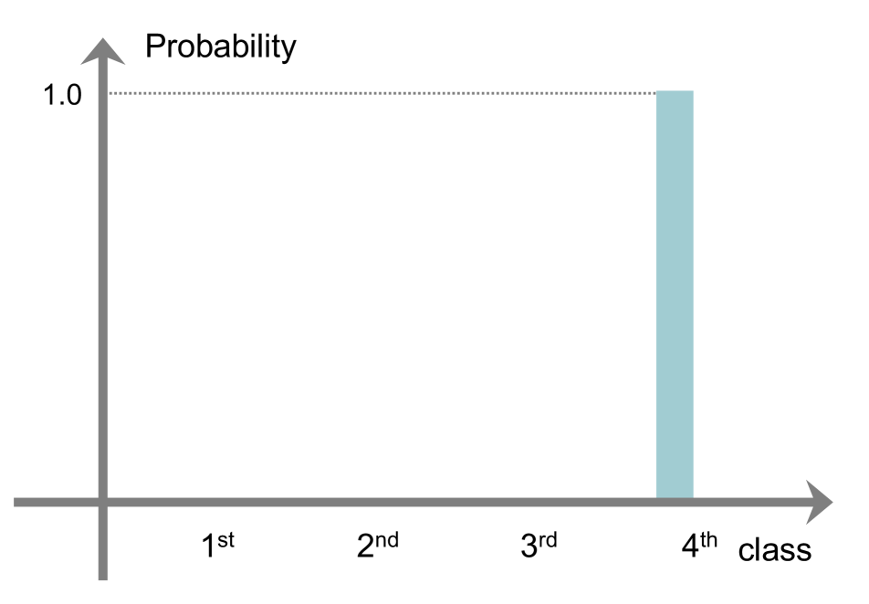
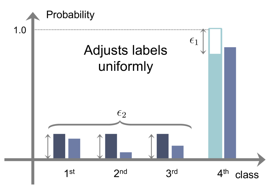
According to and , we can divide existing methods into three groups: AR, CR, and a combination of them (ACR). We illustrate in Fig. 1 the behavior of each regularization method on calibrating output probabilities. Given softmax probabilities and a target distribution (i.e., training labels), LS [32] uniformly adjusts the distribution with hyperparameters, i.e., and (Fig. 1(c)). That is, it uses a constant smoothing function without an indicator function (See the first row in Table 2). FLSD [26], which is a variant of LS, also adopts a uniform smoothing function (See the second row in Table 2).
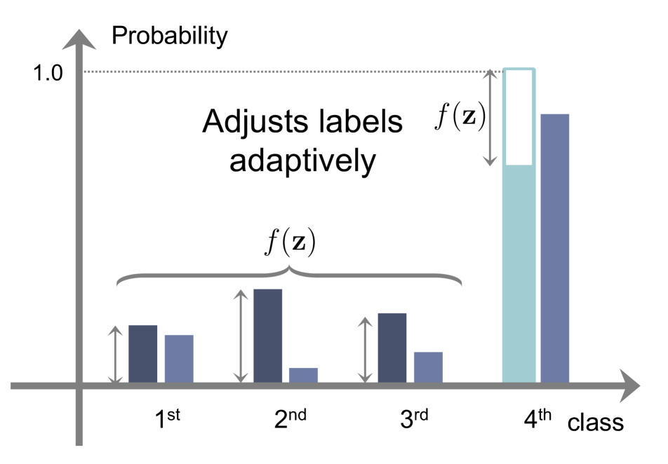
AR.
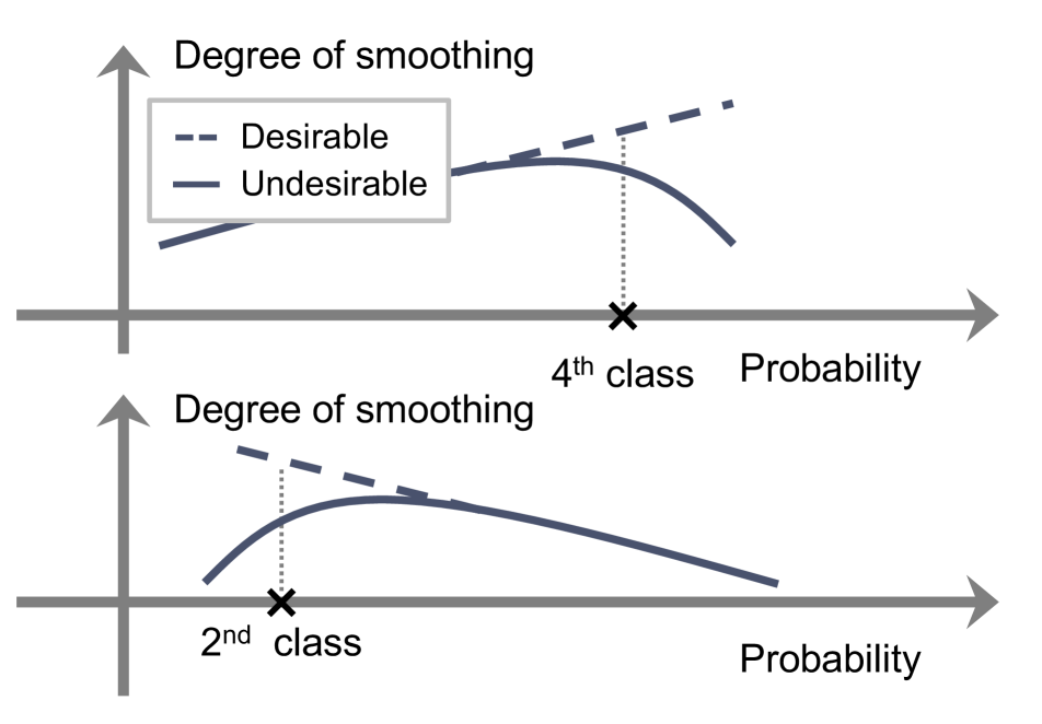
In contrast to LS [32], AR methods use an adaptive smoothing function. We can see in Fig. 1(d) that they adjust the degree of smoothing non-uniformly according to logit values. For example, the smoothing function increases in proportion to the logits, if , reducing the target labels of in Eq. (8) (e.g., the fourth class in Fig. 1(d)). For , the smoothing function raises the target labels of in Eq. (8) in accordance with the logits (e.g., from the first to third classes in Fig. 1(d)). In this case, the probabilities for the corresponding classes increase, making the probability of a network prediction, , relatively small. This reduces the overconfident probability (e.g., in Fig. 1(d)) more effectively than LS. However, we have observed that the smoothing function of AR often violates the desirable behaviors. For example, the smoothing function of MDCA [12] has a parabolic form, which is problematic. When the logit (or the softmax probability of ) is extremely large for (the top in Fig. 1(e)), MDCA rather lessens the degree of smoothing, even worsening the overconfidence problem. Similarly, it lessens the degree of smoothing, when the logit is very small for (the bottom in Fig. 1(e)). CPC [3] outputs negative values when . This in turn raises the target label of the overconfident probability, lessening the degree of smoothing and disturbing a calibration process.
CR.
Instead of using adaptive smoothing functions, a CR method [19] adopts a constant function as in LS [32], and performs label smoothing for miscalibrated probabilities only. In particular, it exploits a specific condition as follows:
| (9) |
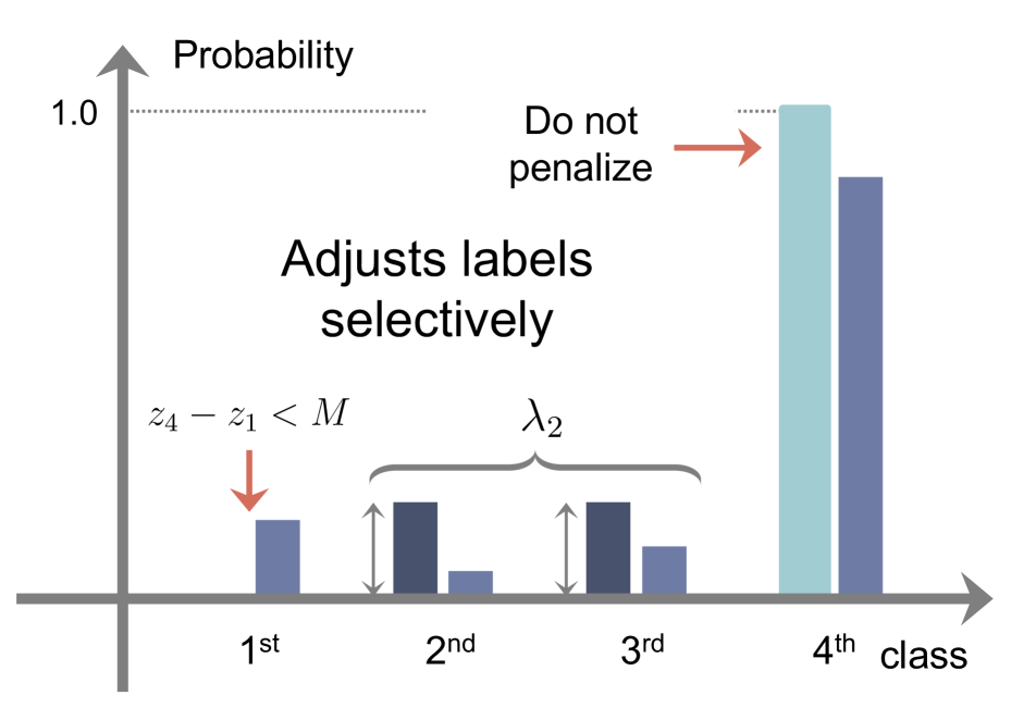
where is a margin and we denote by a function whose output is 1 when the argument is true, and otherwise. We can see that the CR method [19] raises the target labels of in Eq. (8) only if is larger than the margin for . In other words, it determines that the probabilities , where , are well-calibrated, if the logit difference between the network prediction and other classes is smaller than the margin , and applies regularization for miscalibrated probabilities selectively. For example, the first class in Fig. 1(f) does not satisfy the condition in Eq. (9), and thus regularization is not applied, while label smoothing is employed by the amount of for the second and third classes (See Table 2). However, the CR method [19] does not penalize the target label for the class (i.e., for ) directly. This degrades the calibration performance, since the overconfidence problem is likely to occur in the largest probability of (e.g., the fourth class in Fig 1(f)). Note that applying the softmax across for all in the CR method [19] could lower the probability of for the class implicitly. However, by reducing the target label of the class explicitly, while raising the labels of other classes , similar to AR and ACR, we can lower the overconfident probability of more effectively, mitigating the overconfidence problem.
ACR.
CRL [25] has the merits of both AR and CR, adaptively penalizing target labels and preserving well-calibrated probabilities. However, it also inherits the drawback of AR. For example, the smoothing function of CRL [25] has a parabolic form, when and , which is the same as the function of MDCA [12]. This violates the desirable behaviors of the smoothing function (See the top in Fig. 1(e)). Note that the indicator function of CRL uses an ordinal ranking condition [4]. The ranking criterion first records how many times each sample is classified correctly during training (i.e., correctness). It then compares the ordinal ranking relationship based on the correctness by exploiting a ranking loss [35]. At the early phase of training, the correctness history is empty. Networks are thus trained using the CE loss only, causing the overconfidence problem. Moreover, the correctness increases, as the training process goes on. The ranking condition of the indicator function is thus easily not satisfied, making the regularizer inactive and degrading the calibration performance (See Sec 4.3).
3.3 ACLS
We propose novel smoothing and indicator functions that avoid the negative effects of AR and CR, while retaining the advantages of both approaches.
Smoothing function.
To address the limitation of AR [12, 3], we set a smoothing function:
| (10) |
where and are hyperparameters for and terms, respectively. For , our smoothing function provides outputs proportional to the logit values , as it is piecewise linear w.r.t . This indicates that our target label in Eq. (8), i.e., , decreases with an increment of the logit , thereby lowering the probability . Similarly, if , the smoothing function outputs larger values, in accordance with the decrement in the logit , which in turn raises the target label, i.e., , and the probability . In summary, the piecewise linearity in our smoothing function enables always lowering the target label, as the probability increases, and vice versa for other cases consistently, alleviating the limitation of AR.
Indicator function.
We design an indicator function of the gradients in Eq. (8) as follows:
| (11) |
For , we adopt the margin criterion for MbLS [19] to avoid the limitations of an ordinal ranking condition. Different from MbLS, we also use an indicator function for , enabling adjusting the target label for the class , where the overconfidence problem is likely to occur. Specifically, when , the indicator function is , if the difference between maximum and minimum logits is greater than the margin , addressing the overconfidence problem of MbLS.
Training.
ACLS for network calibration.
Regularizers for network calibration satisfy the following conditions: (1) They could lower a probability of for a class , i.e., the largest probability across classes, where the overconfidence problem is likely to occur. (2) They should penalize the probability of selectively, only when it is miscalibrated, since the overconfidence problem for does not always occur. ACLS in Eq. (13) satisfies these conditions. Specifically, it can reduce a logit for the class , lowering the probability of for the class , and vice versa for other classes. The ReLU function with the margin determines whether to adjust the labels, regularizing logit values selectively.
| Dataset | CIFAR10 | Tiny-ImageNet | ImageNet | ||||||||||||
|---|---|---|---|---|---|---|---|---|---|---|---|---|---|---|---|
| ResNet-50 | ResNet-101 | ResNet-50 | ResNet-101 | ResNet-50 | |||||||||||
| ACC | ECE | AECE | ACC | ECE | AECE | ACC | ECE | AECE | ACC | ECE | AECE | ACC | ECE | AECE | |
| CE | 93.20 | 5.85 | 5.84 | 93.33 | 5.74 | 5.73 | 65.02 | 3.73 | 3.69 | 65.62 | 4.97 | 4.97 | 73.96 | 9.10 | 9.24 |
| CE+TS111We use the temperature scaling (TS) method [10], where temperature is optimized on the held-out validation splits. In our experiments, the optimal temperatures are 2.9, 1.1, and 1.4 for ResNet-50 on CIFAR10, Tiny-ImageNet, and ImageNet, and 2.9 and 1.1 for ResNet-101 on CIFAR-10 and Tiny-ImageNet, respectively. [10] | 93.20 | 3.68 | 3.67 | 93.33 | 3.62 | 3.62 | 65.02 | 1.63 | 1.52 | 65.62 | 2.08 | 2.03 | 73.96 | 1.86 | 1.90 |
| MMCE [16] | 95.18 | 3.10 | 3.10 | 94.99 | 3.61 | 3.61 | 64.75 | 5.15 | 5.12 | 65.92 | 4.88 | 4.88 | 74.36 | 8.75 | 8.75 |
| ECP [29] | 94.75 | 3.01 | 2.99 | 93.35 | 5.41 | 5.40 | 64.98 | 4.00 | 3.92 | 65.69 | 4.68 | 4.66 | 73.84 | 8.63 | 8.63 |
| LS [32] | 94.87 | 2.79 | 3.85 | 93.23 | 3.56 | 4.68 | 65.78 | 3.17 | 3.16 | 65.87 | 2.20 | 2.21 | 75.24 | 2.33 | 2.43 |
| FL [18] | 94.82 | 3.90 | 3.86 | 92.42 | 4.60 | 4.58 | 63.09 | 2.96 | 3.12 | 62.97 | 2.55 | 2.44 | 71.76 | 1.79 | 1.79 |
| FLSD [26] | 94.77 | 3.84 | 3.60 | 92.38 | 4.58 | 4.57 | 64.09 | 2.91 | 2.95 | 62.96 | 4.91 | 4.91 | 72.19 | 1.82 | 1.86 |
| MDCA [12] | 94.84 | 6.86 | 6.73 | 95.66 | 6.88 | 7.23 | 63.57 | 2.77 | 2.61 | 66.34 | 6.06 | 6.06 | 75.65 | 7.45 | 7.53 |
| CPC [3] | 95.04 | 3.91 | 3.91 | 95.36 | 3.78 | 3.75 | 65.44 | 3.12 | 3.05 | 66.56 | 3.90 | 4.00 | 75.76 | 4.80 | 4.82 |
| MbLS [19] | 95.25 | 1.16 | 3.18 | 95.13 | 1.38 | 3.25 | 64.74 | 1.64 | 1.73 | 65.81 | 1.62 | 1.68 | 75.39 | 4.07 | 4.14 |
| CRL [25] | 95.08 | 3.14 | 3.11 | 95.04 | 3.74 | 3.73 | 64.88 | 1.65 | 1.52 | 65.87 | 3.57 | 3.56 | 73.83 | 8.47 | 8.47 |
| ACLS | 95.40 | 1.12 | 2.87 | 95.34 | 1.36 | 3.25 | 64.84 | 1.05 | 1.03 | 65.78 | 1.11 | 1.15 | 75.65 | 1.02 | 1.20 |
4 Experiments
In this section, we describe implementation details (Sec 4.1) and compare our approach with the state of the art on image classification and semantic segmentation in terms of calibration metrics (Sec. 4.2). We also provide a detailed analysis of our loss function (Sec 4.3).
4.1 Implementation details.
Datasets and evaluation.
We evaluate our method on CIFAR10 [15], Tiny-ImageNet [17], ImageNet [5] for image classification, and PASCAL VOC [7] for semantic segmentation. The CIFAR10 dataset consists of 50K training and 10K test images of size for 10 classes. Tiny-ImageNet is a subset of ImageNet, and provides 100K training, 10K validation, and 10K test images of 200 classes, where all images are downsampled to the size of from ImageNet. The ImageNet dataset provides approximately 1.2M training and 50K validation images of 1K classes. PASCAL VOC presents 10,582 training and 1,449 validation samples. Following the standard protocol in [10, 26, 19, 12, 25, 24], we report expected calibration error (ECE (%)), adaptive ECE (AECE (%)), and top-1 accuracy (ACC (%)) for image classification. For semantic segmentation, we report ECE (%), AECE (%), and mIoU (%).
Training.
We use network architectures of ResNet-50 and ResNet-101 [11] on CIFAR10 [15] and Tiny-ImageNet [17]. For these datasets, we train the networks using the SGD optimizer with learning rate, weight decay, and momentum of 0.1, 5e-4, and 0.9, respectively. The networks are trained for 350 and 100 epochs with a batch size of 128 and 64 for CIFAR10 and Tiny-ImageNet, respectively. We divide the learning rate by 10 at 150 and 250 epochs for CIFAR10 and at 40 and 60 epochs for Tiny-ImageNet. We train our models with a single NVIDIA RTX A5000 GPU. For ImageNet [5], we train ResNet-50 for 200 epochs using the AdamW optimizer [21], with batch size, learning rate, weight decay, , and of 256, 5e-4, 5e-2, 0.9, and 0.999, respectively. We use a cosine annealing technique [20] as a learning rate scheduler, and train the network with four NVIDIA RTX A5000 GPUs. For semantic segmentation, we follow the experimental protocol in MbLS [19]. We use DeepLabV3 [2] with ImageNet pretrained ResNet-50 as a backbone and train the model with a single NVIDIA RTX A5000 GPU. We train the entire model using the SGD optimizer for 100 epochs with batch size, learning rate, momentum, and weight decay of 8, 1e-2, 0.9, and 5e-4, respectively. We divide the learning rate by 10 at 40 and 80 epochs.
Hyperparameters.
We set the margin to 6 for CIFAR10, and 10 for other datasets, following [19]. To set the hyperparameters and in Eq. (10), we first divide 10% of the training samples for each dataset as a cross-validation split. We then perform a grid search on the split, and set the values of 0.1 and 0.01 for and , respectively. For other regularization-based methods [3, 26, 32, 12, 19, 25], we use default hyperparameters, provided by the authors. We provide a detailed analysis on these parameters in the supplementary material.
4.2 Results
| Method | mIoU | ECE | AECE |
|---|---|---|---|
| CE | 70.92 | 8.26 | 8.23 |
| ECP [29] | 71.16 | 8.31 | 8.26 |
| LS [32] | 71.00 | 9.35 | 9.95 |
| FL [18] | 69.99 | 11.44 | 11.43 |
| MbLS [19] | 71.20 | 7.94 | 7.99 |
| ACLS | 70.63 | 7.29 | 7.28 |
We show in Table 3 quantitative comparisons between our method with state-of-the-art network calibration methods [16, 29, 32, 18, 26, 25, 12, 3, 19] on image classification. For CIFAR10 [15] and Tiny-ImageNet [17], the numbers for the methods [29, 32, 18, 26, 19] are taken from MbLS [19]. For a fair comparison, we reproduce the results of MMCE [16], CRL [25], CPC [3], and MDCA [12] with the same experimental configuration, including network architectures and datasets. For ImageNet [5], we reproduce all the methods in Table 3 with ResNet-50 [11]. From Table 3, we can clearly see that ACLS outperforms all previous calibration methods by significant margins on all benchmarks in terms of ECE and AECE. In particular, we have three findings as follows: (1) ACLS outperforms the AR methods [12, 3] by large margins. MDCA [12] and CPC [3] penalize target labels using adaptive smoothing functions, but they often behave undesirably in terms of network calibration. ACLS addresses this limitation, providing better ECE and AECE, compared with the AR methods. (2) The CR method, MbLS [19], regularizes confidence values selectively. However, it does not penalize the target labels of predicted classes, outperformed by ACLS on all benchmarks. (3) ACLS alleviates the limitations of AR and CR, and it also surpasses CRL [25] in terms of ECE and AECE. We provide in Table 4 quantitative results of semantic segmentation on PASCAL VOC [7]. We can see that our approach outperforms other methods in terms of network calibration, suggesting that it also works well for the dense prediction task.
4.3 Discussion
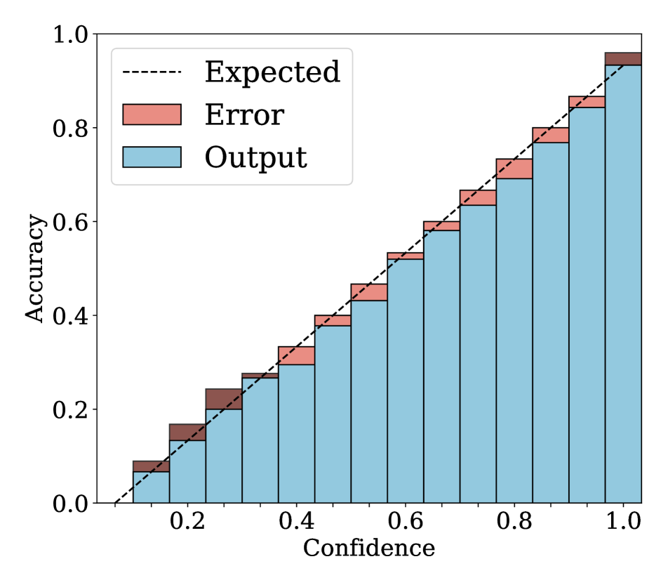
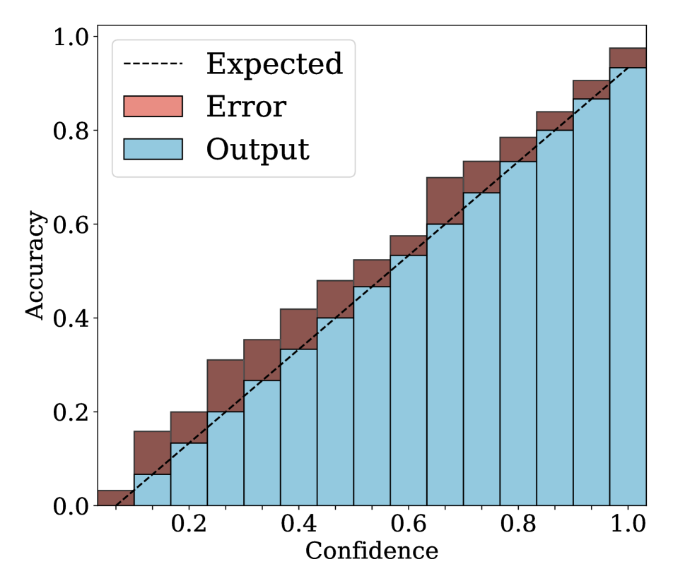
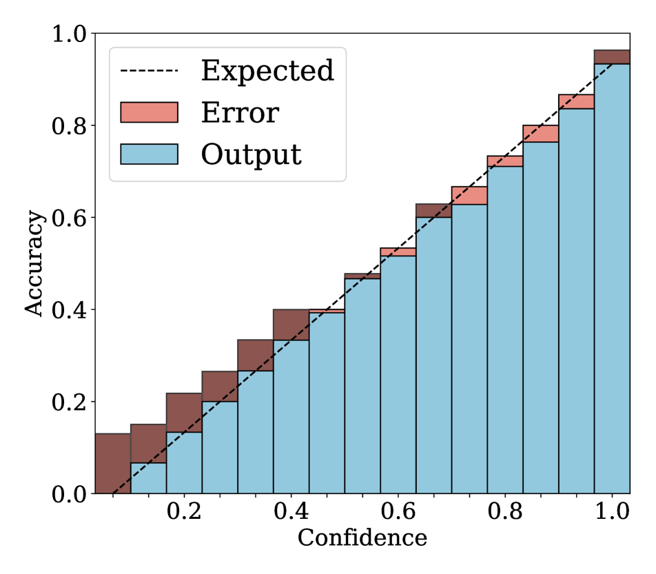
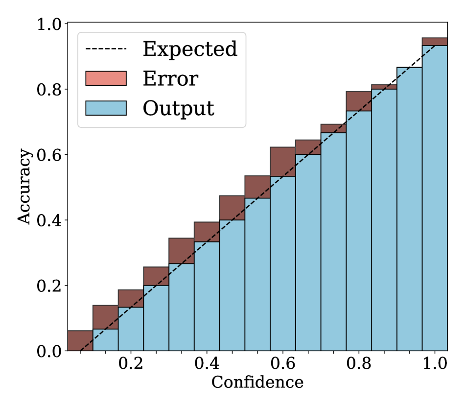
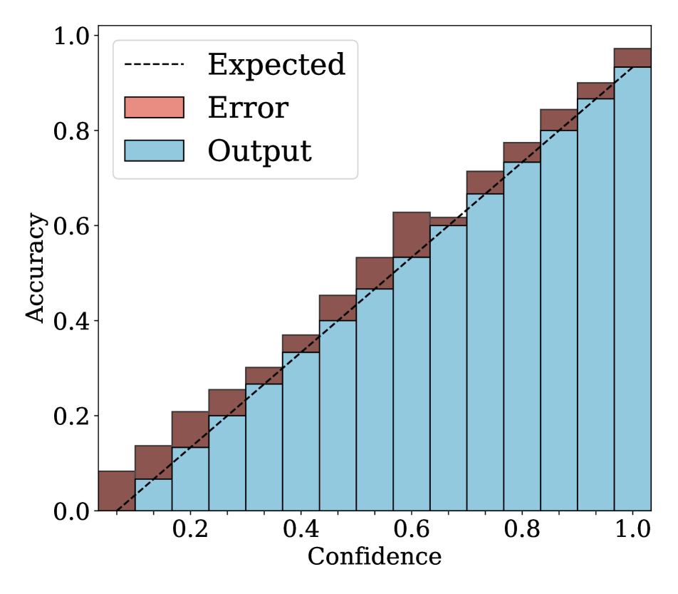
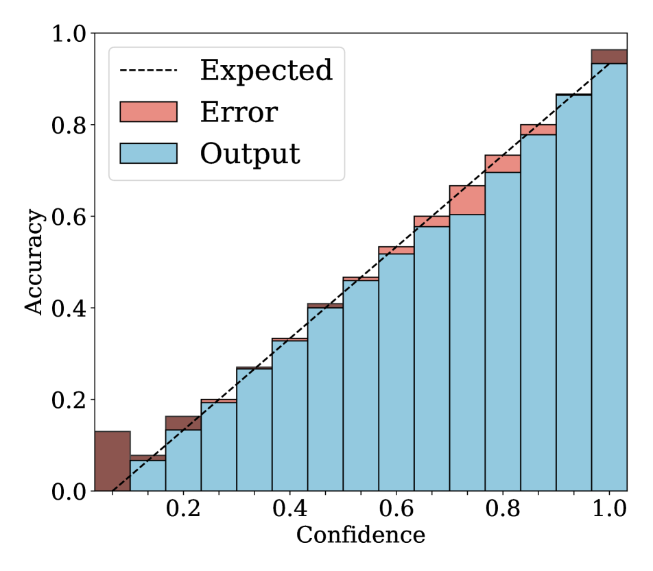
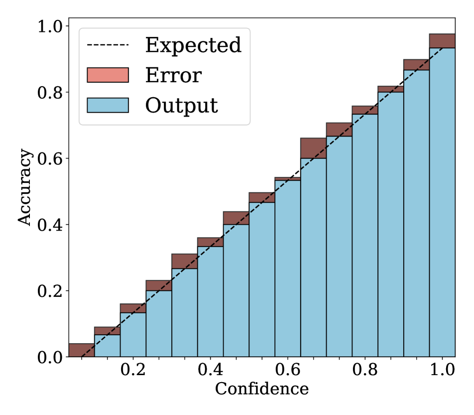
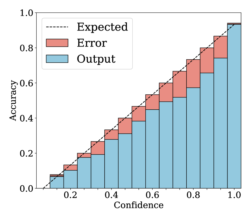
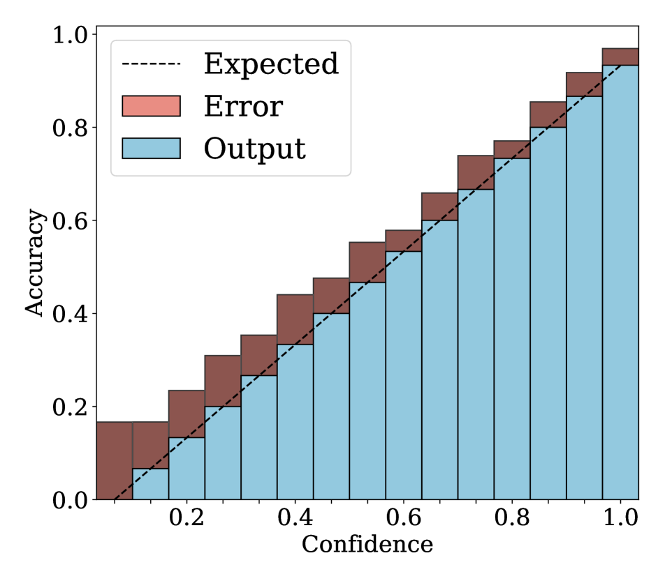
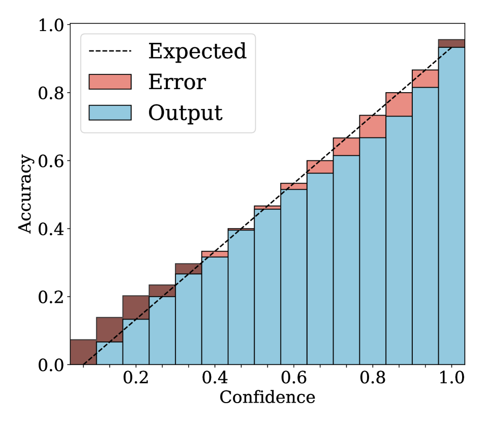
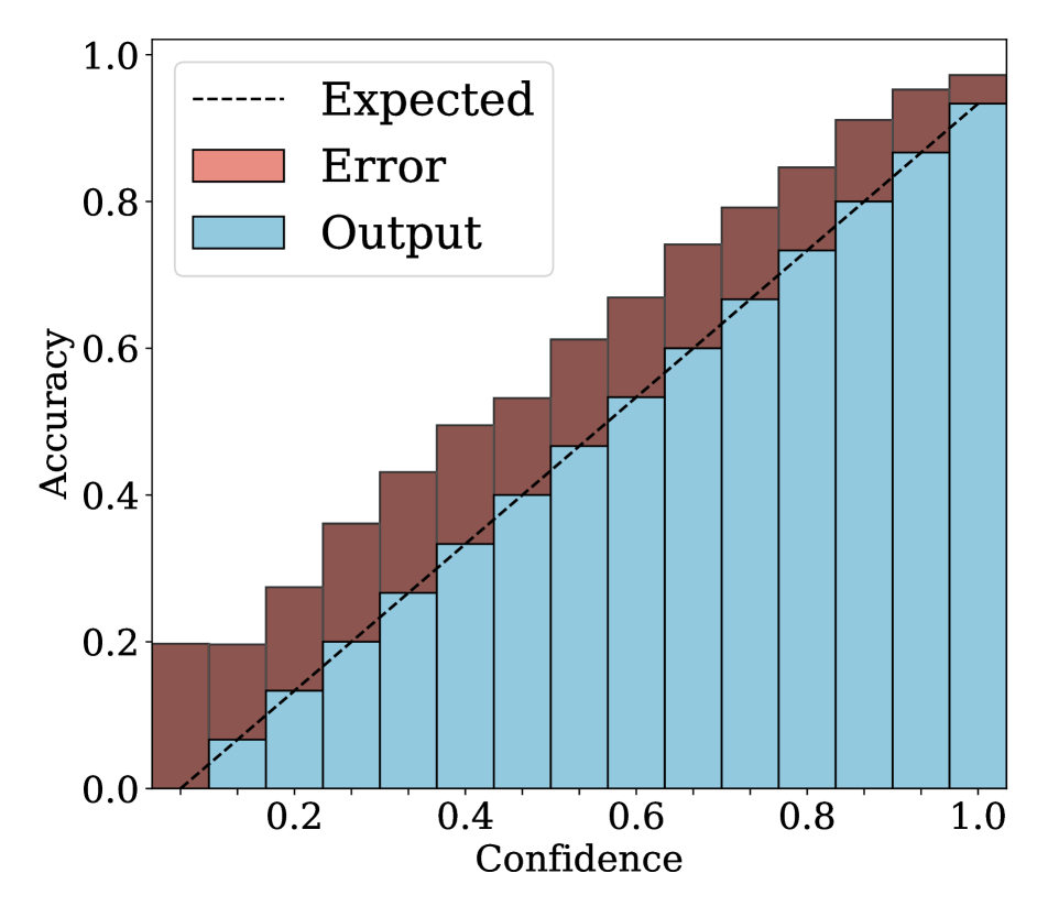
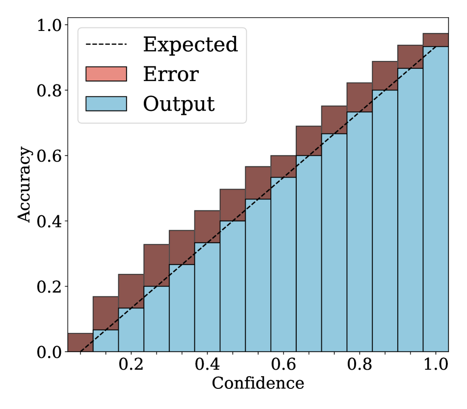
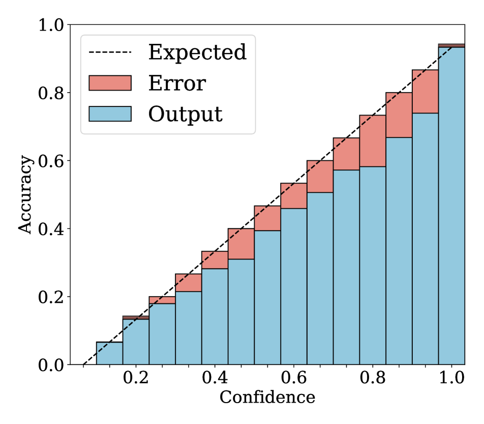
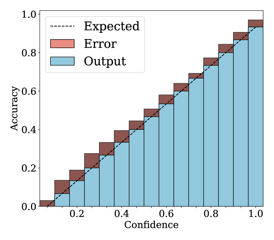
Reliability diagrams.
We show in Fig. 2 reliability diagrams on Tiny-ImageNet [17] and ImageNet [5]. Following the works of [26, 3, 19, 12, 25, 10, 8, 6, 22], we visualize the reliability diagrams of average accuracies and confidences for 15 bins. We can see from Fig. 2 that ACLS outperforms the other methods [32, 19, 3, 12, 25] across the ranges of confidence. Specifically, we can see from the third, fourth, and last columns, ACLS shows better calibration capability than the AR method [12, 3], since they often behave in opposition to the desirable smoothing function, in terms of network calibration situation (See Sec. 3.2). The fifth and last columns show that the CR method (MbLS [19]) provides larger values of confidences, compared to ACLS, across all bins. A plausible reason is that it does not penalize target labels when as in Eq. (9). We can see from the last two columns ACLS surpasses the ACR method [25] since ACLS alleivates the limitations of AR and CR.
| Method | AR | CR | ResNet-50 | ResNet-101 | ||
| ECE | AECE | ECE | AECE | |||
| LS [32] | 3.17 | 3.16 | 2.20 | 2.21 | ||
| MDCA [12] | 2.77 | 2.61 | 6.06 | 6.06 | ||
| Ours (AR only) | 1.54 | 1.42 | 1.34 | 0.89 | ||
| MbLS [19] | 1.64 | 1.73 | 1.62 | 1.68 | ||
| Ours (CR only) | 1.32 | 1.43 | 1.38 | 1.41 | ||
| Ours (ACLS) | 1.05 | 1.03 | 1.11 | 1.15 | ||
Ablation study on AR and CR.
We show in Table 5 an ablation analysis of variant of regularization methods on Tiny-ImageNet [17]. The third and fifth rows show the results of our method that use either a smoothing function of Eq. (10) or an indicator function of Eq. (11) only. From the table, we have the following observations: (1) AR and CR outperform LS by significant margins for both networks. This demonstrates that our smoothing and indicator functions in Eqs. (10) and (11) alleviate the miscalibration remarkably (See the first, third, and fifth rows). (2) We can clearly see that our smoothing function alleviates the limitation of previous AR methods [12, 3] by large margins (See the second and third rows). (3) The indicator function in Eq. (11) surpasses LS and MbLS for both architectures. This suggests that our indicator function calibrates the network more effectively than LS and MbLS (See the first, fourth, and fifth rows). (4) ACLS achieves the best performance, demonstrating that AR and CR are complementary to each other.
Ablation study on conditions.
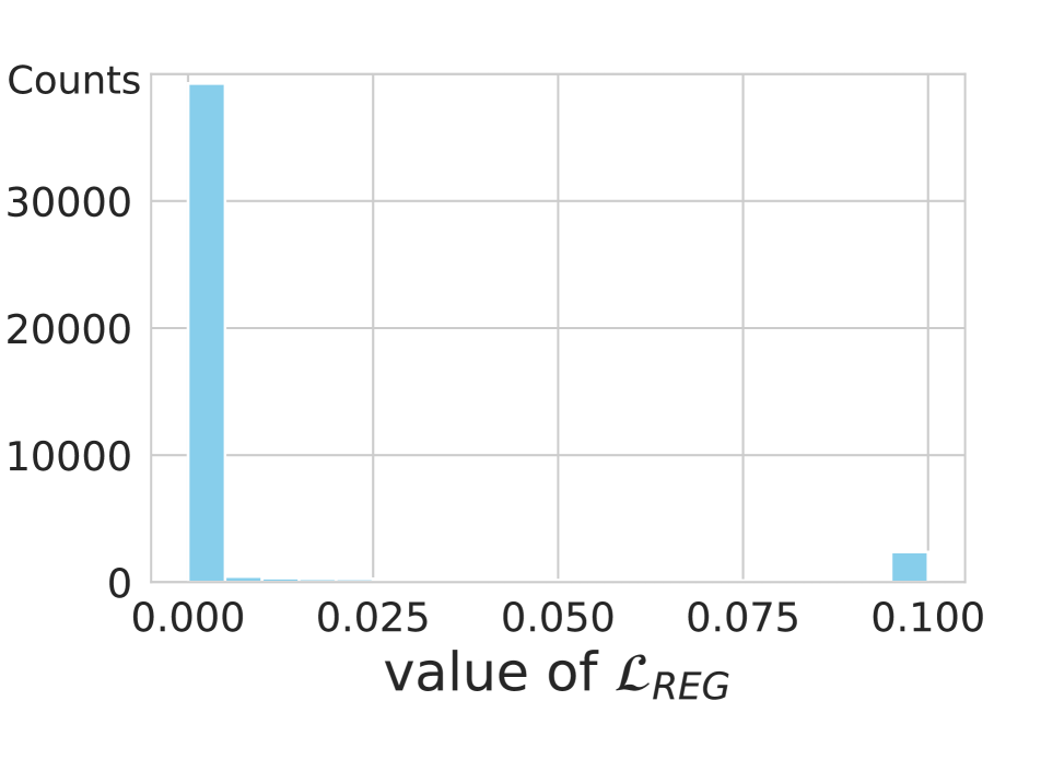
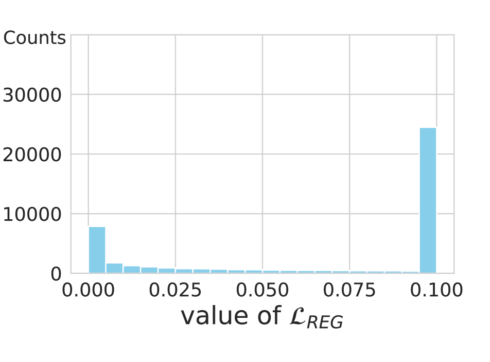
We compare in Table 6 ECE and AECE for indicator functions with margin or ranking conditions. To simulate the result in the second row, we set an indicator function as in Eq. (11), instead of using the original ranking counterpart in CRL [25]. Similarly, we use the ranking condition in CRL [25] for the third row. From the table, we have two findings: (1) For both CRL and ACLS, the methods exploiting the margin condition outperform the ranking counterparts consistently, demonstrating that the margin is more effective than the ranking condition in terms of network calibration as described in Sec. 3.2. The ranking condition compares the ordinal ranking relationship based on the correctness of each sample, where the correctness values are computed by counting the number of correct classifications for each sample during training. At the late phase of training, each sample has similar correctness value, suggesting that the the ordinal ranking relationship will not be satisfied, and preventing regularization. We can see from Fig. 3 that the regularizer is inactive (i.e., ) for 85% of samples, when exploiting ranking conditions (left), while only for 5% of samples for the margin condition (right). Furthermore, at the early phase of training, the correctness history is empty, and thus the networks are trained using softmax CE loss only. This also degrades the calibration of networks. (2) With the same condition, ACLS always outperforms CRL. This demonstrates once again that CRL still suffers from the limitation of AR, while ACLS mitigates the problem.
| Ranking | Margin | ECE | AECE | |
|---|---|---|---|---|
| CRL [25] | 1.65 | 1.52 | ||
| 1.47 | 1.40 | |||
| Ours (ACLS) | 1.48 | 1.19 | ||
| 1.05 | 1.03 |
Limitation.
Similar to other regularization-based calibration methods [3, 12, 18, 19, 26, 25], ACLS requires re-training networks from scratch, which is computationally expensive. Also, ACLS might not behave as expected for an exceptional case. Let us suppose the case of , i.e., and , and assume that and are sufficiently large and small, respectively, and . ACLS tries to reduce , since is large enough. The ordering for and could then be altered, i.e., , which in turn changes the prediction after a backward pass (i.e., from ). This might degrade the classification performance. We have observed that this altering occurs in 0.29% of samples during the last epoch of training on Tiny-ImageNet [17].
5 Conclusion
We have provided an in-depth analysis on existing calibration methods, and have found that they can be interpreted as variants of label smoothing. Based on this, we have presented a new regularization term for network calibration, dubbed ACLS, that addresses both overconfidence and underconfidence problems effectively. Finally, we have shown that our approach sets a new state of the art on standard calibration benchmarks.
Acknowledgments. This work was partly supported by IITP grant funded by the Korea government (MSIT) (No.RS-2022-00143524, Development of Fundamental Technology and Integrated Solution for Next-Generation Automatic Artificial Intelligence System, No.2022-0-00124, Development of Artificial Intelligence Technology for Self-Improving Competency-Aware Learning Capabilities) and the KIST Institutional Program (Project No.2E31051-21-203).
References
- [1] Gustavo Carneiro, Leonardo Zorron Cheng Tao Pu, Rajvinder Singh, and Alastair Burt. Deep learning uncertainty and confidence calibration for the five-class polyp classification from colonoscopy. Medical image analysis, 62:101653, 2020.
- [2] Liang-Chieh Chen, George Papandreou, Florian Schroff, and Hartwig Adam. Rethinking atrous convolution for semantic image segmentation. arXiv preprint arXiv:1706.05587, 2017.
- [3] Jiacheng Cheng and Nuno Vasconcelos. Calibrating deep neural networks by pairwise constraints. In CVPR, 2022.
- [4] Charles Corbière, Nicolas Thome, Avner Bar-Hen, Matthieu Cord, and Patrick Pérez. Addressing failure prediction by learning model confidence. In NeurIPS, 2019.
- [5] Jia Deng, Wei Dong, Richard Socher, Li-Jia Li, Kai Li, and Li Fei-Fei. Imagenet: A large-scale hierarchical image database. In CVPR, 2009.
- [6] Zhipeng Ding, Xu Han, Peirong Liu, and Marc Niethammer. Local temperature scaling for probability calibration. In ICCV, 2021.
- [7] Mark Everingham, Luc Van Gool, Christopher KI Williams, John Winn, and Andrew Zisserman. The pascal visual object classes (voc) challenge. IJCV, 88:303–308, 2009.
- [8] Arindam Ghosh, Thomas Schaaf, and Matt Gormley. Adafocal: Calibration-aware adaptive focal loss. In NeurIPS, 2022.
- [9] Sorin Grigorescu, Bogdan Trasnea, Tiberiu Cocias, and Gigel Macesanu. A survey of deep learning techniques for autonomous driving. Journal of Field Robotics, 37:362–386, 2020.
- [10] Chuan Guo, Geoff Pleiss, Yu Sun, and Kilian Q Weinberger. On calibration of modern neural networks. In ICML, 2017.
- [11] Kaiming He, Xiangyu Zhang, Shaoqing Ren, and Jian Sun. Deep residual learning for image recognition. In CVPR, 2016.
- [12] Ramya Hebbalaguppe, Jatin Prakash, Neelabh Madan, and Chetan Arora. A stitch in time saves nine: A train-time regularizing loss for improved neural network calibration. In CVPR, 2022.
- [13] Tove Helldin, Göran Falkman, Maria Riveiro, and Staffan Davidsson. Presenting system uncertainty in automotive uis for supporting trust calibration in autonomous driving. In AutomotiveUI, 2013.
- [14] Xiaoqian Jiang, Melanie Osl, Jihoon Kim, and Lucila Ohno-Machado. Calibrating predictive model estimates to support personalized medicine. Journal of the American Medical Informatics Association, 19:263–274, 2012.
- [15] Alex Krizhevsky, Geoffrey Hinton, et al. Learning multiple layers of features from tiny images. Technical report, 2009.
- [16] Aviral Kumar, Sunita Sarawagi, and Ujjwal Jain. Trainable calibration measures for neural networks from kernel mean embeddings. In ICML, 2018.
- [17] Ya Le and Xuan Yang. Tiny imagenet visual recognition challenge. CS 231N, 2015.
- [18] Tsung-Yi Lin, Priya Goyal, Ross Girshick, Kaiming He, and Piotr Dollár. Focal loss for dense object detection. In ICCV, 2017.
- [19] Bingyuan Liu, Ismail Ben Ayed, Adrian Galdran, and Jose Dolz. The devil is in the margin: Margin-based label smoothing for network calibration. In CVPR, 2022.
- [20] Ilya Loshchilov and Frank Hutter. Sgdr: Stochastic gradient descent with warm restarts. arXiv preprint arXiv:1608.03983, 2016.
- [21] Ilya Loshchilov and Frank Hutter. Decoupled weight decay regularization. arXiv preprint arXiv:1711.05101, 2017.
- [22] Xingchen Ma and Matthew B Blaschko. Meta-cal: Well-controlled post-hoc calibration by ranking. In ICML, 2021.
- [23] Alireza Mehrtash, William M Wells, Clare M Tempany, Purang Abolmaesumi, and Tina Kapur. Confidence calibration and predictive uncertainty estimation for deep medical image segmentation. IEEE transactions on medical imaging, 39:3868–3878, 2020.
- [24] Matthias Minderer, Josip Djolonga, Rob Romijnders, Frances Hubis, Xiaohua Zhai, Neil Houlsby, Dustin Tran, and Mario Lucic. Revisiting the calibration of modern neural networks. In NeurIPS, 2021.
- [25] Jooyoung Moon, Jihyo Kim, Younghak Shin, and Sangheum Hwang. Confidence-aware learning for deep neural networks. In ICML, 2020.
- [26] Jishnu Mukhoti, Viveka Kulharia, Amartya Sanyal, Stuart Golodetz, Philip Torr, and Puneet Dokania. Calibrating deep neural networks using focal loss. In NeurIPS, 2020.
- [27] Rafael Müller, Simon Kornblith, and Geoffrey E Hinton. When does label smoothing help? In NeurIPS, 2019.
- [28] Jeremy Nixon, Michael W Dusenberry, Linchuan Zhang, Ghassen Jerfel, and Dustin Tran. Measuring calibration in deep learning. In CVPRW, 2019.
- [29] Gabriel Pereyra, George Tucker, Jan Chorowski, Łukasz Kaiser, and Geoffrey Hinton. Regularizing neural networks by penalizing confident output distributions. In ICLRW, 2017.
- [30] John Platt et al. Probabilistic outputs for support vector machines and comparisons to regularized likelihood methods. Advances in large margin classifiers, 10:61–74, 1999.
- [31] Andrea Stocco, Michael Weiss, Marco Calzana, and Paolo Tonella. Misbehaviour prediction for autonomous driving systems. In ICSE, 2020.
- [32] Christian Szegedy, Vincent Vanhoucke, Sergey Ioffe, Jon Shlens, and Zbigniew Wojna. Rethinking the inception architecture for computer vision. In CVPR, 2016.
- [33] Christian Tomani, Daniel Cremers, and Florian Buettner. Parameterized temperature scaling for boosting the expressive power in post-hoc uncertainty calibration. In ECCV, 2022.
- [34] Deng-Bao Wang, Lei Feng, and Min-Ling Zhang. Rethinking calibration of deep neural networks: Do not be afraid of overconfidence. In NeurIPS, 2021.
- [35] Jiang Wang, Yang Song, Thomas Leung, Chuck Rosenberg, Jingbin Wang, James Philbin, Bo Chen, and Ying Wu. Learning fine-grained image similarity with deep ranking. In CVPR, 2014.
- [36] Jize Zhang, Bhavya Kailkhura, and T Yong-Jin Han. Mix-n-match: Ensemble and compositional methods for uncertainty calibration in deep learning. In ICML, 2020.
See pages 1 of camera-ready-supp.pdf See pages 2 of camera-ready-supp.pdf See pages 3 of camera-ready-supp.pdf See pages 4 of camera-ready-supp.pdf See pages 5 of camera-ready-supp.pdf