Acoustic anomaly Detection via Latent Regularized Gaussian Mixture Generative Adversarial Networks

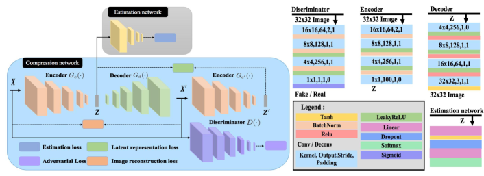
Inspired by the anomaly detection methods [11, 12, 13, 14], proposed architecture is shown in Fig. 1, consists of two subnetworks: compression network and estimation network.

We define a loss function in Eqn. (1) including four components, $i.e.$, the image reconstruction loss $\mathcal{L}_{irec}$, the adversarial loss $\mathcal{L}_{adv}$, the latent representation loss $\mathcal{L}_{zrec}$ and the estimation loss $\mathcal{L}_{es}:$

$$\mathcal{L}=w_{i}\mathcal{L}_{irec}+w_{a}\mathcal{L}_{adv}+w_{z}\mathcal{L}_{zrec}+w_{e}\mathcal{L}_{es}$$

(1)

where $w_{i}$, $w_{a}$, $w_{z}$, and $w_{e}$ are the weighting parameters balancing the impact of individual item to the overall object function.

Adversarial Loss: GAN was first used by Goodfellow [17], which consists of a generator and a discriminator having two competing objectives: the discriminator $D$ is learned to distinguish generated images from original input images, while the generator $G$ is trained to produce realistic images to fool $D$. The training objective of GAN can be formulated as :

	$\displaystyle\mathcal{L}_{adv}=\min_{G}\max_{D}(E_{\boldsymbol{x}\sim p_{\mathbf{x}}}[\log(D(\mathbf{x}))]$		(2)
	$\displaystyle+E_{\boldsymbol{x}\sim p_{\mathbf{x}}}[\log(1-D(G(\mathbf{x})))]).$

Image reconstruction loss: Image reconstruction loss measures the pixel-wise reconstruction error between original input image and generated image, which helps the generator to sufficiently capture the input sample distribution for normal samples. The training objective is shown below:

$$\mathcal{L}_{irec}=\mathbb{E}_{x\sim p_{\mathbf{x}}}\|x-G(x)\|_{1}$$

(3)

Latent representation loss: With the adversarial loss and image reconstruction loss defined above, the model can generate the realistic image. In additional to these objectives, the latent feature of generated image and that of the original input image are also expected to be consistent, which could help the generator to capture the latent feature for common examples. Hence, we consider to add a constraint by minimizing the distance between latent feature of input images $G_{e}(x)$ from generator and encoded latent feature of generated image from auxiliary encoder $G_{e^{\prime}}(x^{\prime})$ as follows.

$$\mathcal{L}_{zrec}=\mathbb{E}_{x\sim p_{\mathbf{X}}}\left\|G_{e}(x)-G_{e^{\prime}}(x^{\prime})\right\|_{2}$$

(4)

Estimation loss: Given the latent representation $z$ from compression network and an integer $K$ as the number of mixture components. The estimation network is a multi-layer network followed by a softmax layer, which makes mixture-component membership prediction as follows:

$${\hat{\gamma}}=\operatorname{softmax}(MLN\left(\mathbf{z};\theta_{m}\right)),$$

where $\hat{\gamma}$ is a $K$-dimensional vector for the soft mixture-component membership prediction, which is the output of the estimation network parameterized by $\theta_{m}$. $\hat{\gamma}_{k}$ denotes the probability of the input sample belongs to the $k^{\text{th }}$ distribution. Given a batch of N samples and their membership prediction, $\forall 1\leq k\leq K$ we can further estimate the parameters in GMM as follows:

	$\displaystyle\hat{\alpha}_{k}=$	$\displaystyle\frac{1}{n}\sum_{i=1}^{n}\hat{\gamma}_{ik};\hat{u}_{k}=\frac{\sum_{i=1}^{n}\hat{\gamma}_{ik}z_{i}}{\sum_{i=1}^{n}\hat{\gamma}_{ik}},$		(5)
	$\displaystyle\hat{\Sigma}_{k}=$	$\displaystyle\frac{\sum_{i=1}^{n}\hat{\gamma}_{ik}\left(z_{i}-\hat{u}_{k}\right)\left(z_{i}-\hat{u}_{k}\right)^{T}}{\sum_{i=1}^{n}\hat{\gamma}_{ik}},$

where $\hat{\alpha}_{k}$, $\hat{u}_{k}$, $\hat{\Sigma}_{k}$ are the $k^{th}$ component mixture weights, , the $k^{th}$ component mixture mean and the $k^{th}$ component mixture covariance. $\hat{\gamma}_{ik}$ is the membership prediction of the $i^{th}$ input sample $z_{i}$. n is the number of input samples. With the GMM parameters, the energy function of an input sample can be formulated as follows:

$$E(\mathbf{z})=-\log\left(\sum_{k=1}^{K}\hat{\phi}_{k}\frac{\exp\left(-\frac{1}{2}\left(\mathbf{z}-\hat{\mu}_{k}\right)^{T}\hat{\mathbf{\Sigma}}_{k}^{-1}\left(\mathbf{z}-\hat{\mu}_{k}\right)\right)}{\sqrt{\left|2\pi\Sigma_{k}\right|}}\right).$$

(6)

The objective function of estimation network is to minimize following equation,

$$\mathcal{L}_{es}=\lambda_{1}\sum_{i=1}^{N}E\left(z_{i}\right)+\lambda_{2}\sum_{k=1}^{K}\sum_{j=1}^{d}\frac{1}{\hat{\Sigma}_{jj}^{k}},$$

(7)

where the first term is the sum of sample energy. The second term is the regularizer, which penalizes small values on the diagonal entries in covariance matrices $\Sigma_{k},k=1,\ldots,K$. The purpose of this measure is to avoid the singularity problem in GMM. $\lambda_{1}$ and $\lambda_{2}$ are the meta parameters in estimation network.

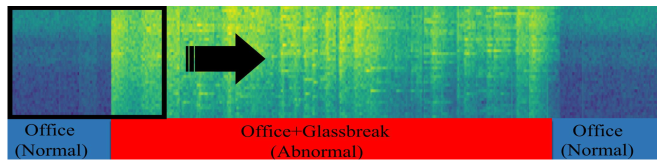
Datasets: We extract 15 datasets from the 2017 DCASE Challenge Task 2 dataset [18], as it is done in [19]. Three different abnormal event exists in this dataset (i.e., gunshot, babycry and glassbreak). All of these abnormal event audios are artificially mixed with background audios respectively which includes 15 different kinds of environmental settings (i.e.,home, bus, and train). Fig. 2 shows the office environment audio mixed with galss-break audio. All acoustic signals are converted to the spectrogram data, which is used as input data for proposed framework.

According to the work [14], CIFAR10 and MNIST dataset are used to construct a toy experiment to illustrate our superiority to other state-of-the-art abnormal detectors. One of classes would be regarded as an normal class, while the rest ones belong to the anomaly class. In total, we get ten sets for MNIST dataset and CIFAR10 dataset.

Evaluation Measures: In testing process, the latent representation loss of each given spectrogram is regarded as an abnormal score. We compute the Area Under the ROC Curve (AUC) to measure the performance of proposed method.

Implementation Details: We implement our approach in PyTorch by optimizing the weighted loss $\mathcal{L}$ (defined in Eq. (1)) with the weight values $w_{i}=1$, $w_{a}=5$, $w_{z}=1$, and $w_{e}=0.05$, which are empirically chosen to yield optimum results.

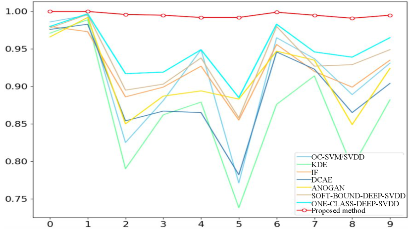
In this subsection, we observe the clear superiority of our approach over previous abnormal detection models (OC-SVM/SVDD [20], KDE [21], IF [22], DCAE[23], ANOGAN [12], DEEP-SVDD [24]), as it is shown in Fig. 3. For each digit chosen as normal class in MNIST dataset, the proposed method achieves the best performance in term of AUC value, which could be illustrated by using red curves. In the right of the Fig. 3, we also present the comparison result in CIFAR10 dataset.

Since all loss functions are presented in subsection 2.2, giving the ablation study to the different combinations of loss functions is necessary. As illustrated in Tab. 1, five background-event experiments are done in the three kinds of loss combinations respectively. Each loss function we designed in the proposed framework can improve the performance.

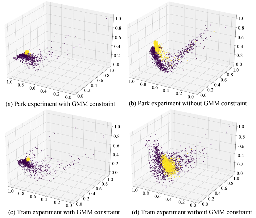
To further explain the necessity of estimation constraint, Fig. 4 presents the visualization of the latent feature, where the proposed method with and without estimation constraint are compared on park and tram experiment setting. To sum up, comparison result can indicate the following: (1) Compared with the model without estimation constraint, the normal samples (yellow dots) are more concentrated with estimation constraint. (2) The anomalous samples can be more separated from normal samples (yellow dots).

The performance of three models across the 15 datasets is shown in Table 2. We find that the proposed model consistently outperforms the other models in almost all datasets, with a tie in the home, cafe/restaurant and residential area scenarios.

References

- [1] Erik Marchi, Fabio Vesperini, Stefano Squartini, and Björn Schuller, “Deep recurrent neural network-based autoencoders for acoustic novelty detection,” Computational intelligence and neuroscience, vol. 2017, 2017.
- [2] Timothy J O’Shea, T Charles Clancy, and Robert W McGwier, “Recurrent neural radio anomaly detection,” arXiv preprint arXiv:1611.00301, 2016.
- [3] Sepp Hochreiter and Jürgen Schmidhuber, “Long short-term memory,” Neural computation, vol. 9, no. 8, pp. 1735–1780, 1997.
- [4] Aaron van den Oord, Sander Dieleman, Heiga Zen, Karen Simonyan, Oriol Vinyals, Alex Graves, Nal Kalchbrenner, Andrew Senior, and Koray Kavukcuoglu, “Wavenet: A generative model for raw audio,” arXiv preprint arXiv:1609.03499, 2016.
- [5] Stavros Ntalampiras, Ilyas Potamitis, and Nikos Fakotakis, “Probabilistic novelty detection for acoustic surveillance under real-world conditions,” IEEE Transactions on Multimedia, vol. 13, no. 4, pp. 713–719, 2011.
- [6] Wei Bao, Jun Yue, and Yulei Rao, “A deep learning framework for financial time series using stacked autoencoders and long-short term memory,” PloS one, vol. 12, no. 7, pp. e0180944, 2017.
- [7] Emanuele Principi, Fabio Vesperini, Stefano Squartini, and Francesco Piazza, “Acoustic novelty detection with adversarial autoencoders,” in 2017 International Joint Conference on Neural Networks (IJCNN). IEEE, 2017, pp. 3324–3330.
- [8] Weining Lu, Yu Cheng, Cao Xiao, Shiyu Chang, Shuai Huang, Bin Liang, and Thomas Huang, “Unsupervised sequential outlier detection with deep architectures,” IEEE transactions on image processing, vol. 26, no. 9, pp. 4321–4330, 2017.
- [9] Dong Oh and Il Yun, “Residual error based anomaly detection using auto-encoder in smd machine sound,” Sensors, vol. 18, no. 5, pp. 1308, 2018.
- [10] Peter J Huber, Robust statistics, Springer, 2011.
- [11] Houssam Zenati, Chuan Sheng Foo, Bruno Lecouat, Gaurav Manek, and Vijay Ramaseshan Chandrasekhar, “Efficient gan-based anomaly detection,” arXiv preprint arXiv:1802.06222, 2018.
- [12] Thomas Schlegl, Philipp Seeböck, Sebastian M Waldstein, Ursula Schmidt-Erfurth, and Georg Langs, “Unsupervised anomaly detection with generative adversarial networks to guide marker discovery,” in International conference on information processing in medical imaging. Springer, 2017, pp. 146–157.
- [13] Dan Li, Dacheng Chen, Jonathan Goh, and See-kiong Ng, “Anomaly detection with generative adversarial networks for multivariate time series,” arXiv preprint arXiv:1809.04758, 2018.
- [14] Samet Akcay, Amir Atapour-Abarghouei, and Toby P Breckon, “Ganomaly: Semi-supervised anomaly detection via adversarial training,” in Asian Conference on Computer Vision. Springer, 2018, pp. 622–637.
- [15] Bo Zong, Qi Song, Martin Renqiang Min, Wei Cheng, Cristian Lumezanu, Daeki Cho, and Haifeng Chen, “Deep autoencoding gaussian mixture model for unsupervised anomaly detection,” 2018.
- [16] Shuangfei Zhai, Yu Cheng, Weining Lu, and Zhongfei Zhang, “Deep structured energy based models for anomaly detection,” arXiv preprint arXiv:1605.07717, 2016.
- [17] Ian Goodfellow, Jean Pouget-Abadie, Mehdi Mirza, Bing Xu, David Warde-Farley, Sherjil Ozair, Aaron Courville, and Yoshua Bengio, “Generative adversarial nets,” in Advances in neural information processing systems, 2014, pp. 2672–2680.
- [18] Annamaria Mesaros, Toni Heittola, Aleksandr Diment, Benjamin Elizalde, Ankit Shah, Emmanuel Vincent, Bhiksha Raj, and Tuomas Virtanen, “Dcase 2017 challenge setup: Tasks, datasets and baseline system,” 2017.
- [19] Ellen Rushe and Brian Mac Namee, “Anomaly detection in raw audio using deep autoregressive networks,” in ICASSP 2019-2019 IEEE International Conference on Acoustics, Speech and Signal Processing (ICASSP). IEEE, 2019, pp. 3597–3601.
- [20] Yunqiang Chen, Xiang Sean Zhou, and Thomas S Huang, “One-class svm for learning in image retrieval,” in Proceedings 2001 International Conference on Image Processing (Cat. No. 01CH37205). IEEE, 2001, vol. 1, pp. 34–37.
- [21] Emanuel Parzen, “On estimation of a probability density function and mode,” The annals of mathematical statistics, vol. 33, no. 3, pp. 1065–1076, 1962.
- [22] Fei Tony Liu, Kai Ming Ting, and Zhi-Hua Zhou, “Isolation forest,” in 2008 Eighth IEEE International Conference on Data Mining. IEEE, 2008, pp. 413–422.
- [23] Jonathan Masci, Ueli Meier, Dan Cireşan, and Jürgen Schmidhuber, “Stacked convolutional auto-encoders for hierarchical feature extraction,” in International conference on artificial neural networks. Springer, 2011, pp. 52–59.
- [24] Lukas Ruff, Robert Vandermeulen, Nico Goernitz, Lucas Deecke, Shoaib Ahmed Siddiqui, Alexander Binder, Emmanuel Müller, and Marius Kloft, “Deep one-class classification,” in International conference on machine learning, 2018, pp. 4393–4402.