Acoustic Pancharatnam-Berry Geometric Phase Induced by Transverse Spin

Wanyue Xiao Department of Physics, City University of Hong Kong, Tat Chee Avenue, Kowloon, Hong Kong, China Wenjian Kuang Division of Science, Engineering and Health Studies, College of Professional and Continuing Education, Hong Kong Polytechnic University, Hong Kong, China Sibo Huang Department of Electrical Engineering, City University of Hong Kong, Tat Chee Avenue, Kowloon, Hong Kong, China Shanjun Liang junot.liang@cpce-polyu.edu.hk Division of Science, Engineering and Health Studies, College of Professional and Continuing Education, Hong Kong Polytechnic University, Hong Kong, China Din Ping Tsai Department of Electrical Engineering, City University of Hong Kong, Tat Chee Avenue, Kowloon, Hong Kong, China Shubo Wang shubwang@cityu.edu.hk Department of Physics, City University of Hong Kong, Tat Chee Avenue, Kowloon, Hong Kong, China

Abstract

Common wisdom believes that the Pancharatnam-Berry (PB) geometric phase is absent in acoustics due to the spin-0 nature of sound waves. We theoretically and experimentally demonstrate that the PB phase can emerge in surface sound waves (SSWs) carrying transverse spin. The phase differs for the SSWs propagating in opposite directions due to spin-momentum locking. We further realize acoustic PB metasurfaces for nearly arbitrary wavefront manipulation. Our work provides the missing piece of acoustic geometric phases, offering new insights into the fundamental properties of sound waves and opening a new avenue for sound manipulation based on the PB phase.

Introduction
Geometric phase arises when the eigenstate of a system undergoes a cyclic evolution in some parameter space [1]. It had a profound impact on physics with an elegant interpretation based on the fiber bundle theory [2]. The geometric phase can reveal intricate topological structures of the state and parameter spaces [3] and give rise to numerous intriguing phenomena, such as the Aharonov–Bohm effect [4], quantum Hall and quantum spin-Hall effects [5, 6, 7], etc. Recently, the geometric phases in classical wave systems have attracted enormous attention. A prominent example is the momentum-space geometric phase in periodic optical and acoustic systems. This type of geometric phase characterizes the topological properties of nontrivial edge or corner states [8, 9], which have applications in robust communications [10, 11], high-efficiency lasing [12, 13], and quantum information processing [14, 15, 16].

In addition to the momentum-space geometric phase, there is another type of geometric phase induced by wave spin, including the spin-redirection phase [17, 18, 19] and the PB phase [20, 21]. The spin-redirection phase arises in the spatial variations of spin direction [22, 23]. It accounts for the optical spin-Hall effect in light reflection or refraction [24, 25, 26] and the spin-dependent vortex generation in light scattering or focusing [27, 28, 29]. The PB phase is attributed to the polarization evolutions induced by anisotropic materials or structures [30, 31]. This geometric phase is crucial to the optical metasurfaces with remarkable applications, such as metalens [32, 33], holographic imaging [34], and nonlinear harmonic generations [35]. Notably, for generic evolutions of optical polarization in three-dimensional real space, the resulting geometric phase comprises both spin-redirection and PB phases, offering important insights into the real-space topological properties of structured lights [36, 37].

Despite the ubiquity of the geometric phases, it is believed that the spin-redirection and PB phases do not exist in acoustics since the sound waves in air or fluids carry no spin. Some interesting analogs have been realized using acoustic vortices, where the orbital angular momentum (OAM) plays the role of spin in inducing the geometric phases [38, 39]. For example, the transport of acoustic vortices in a helical waveguide can give rise to an analog of the spin-redirection phase due to the OAM circulation on the momentum sphere [40]. Also, the interaction between acoustic vortices and meta-structures, which induces the conversion of OAM topological charges, can generate a geometric phase similar to the PB phase [41, 42, 43]. On the other hand, recent research demonstrates that acoustic spin can be assigned to inhomogeneous sound waves with locally rotating velocity fields [44, 45, 46]. An interesting question is: Can the acoustic spin give rise to the geometric phases?

The answer seems to be ‘No’, considering the different nature of light and sound. Light is a transverse wave with two vector field degrees of freedom (i.e., electric field $\mathbf{E}$ and magnetic field $\mathbf{H}$ ) while sound is a longitudinal wave comprising a scalar pressure field $p$ and a vector velocity field $\mathbf{v}$ . Their interactions with matter result in fundamentally different physics. Specifically, the optical PB phase can appear in circularly polarized light interacting with anisotropic structures such as metasurfaces, where the subwavelength meta-atoms induce polarization evolutions through the electric dipole. In contrast, generic sound waves are not circularly polarized globally, and their interaction with subwavelength meta-atoms is usually dominated by the acoustic monopole, which has isotropic mode fields and cannot induce polarization evolutions.

Here, we theoretically and experimentally demonstrate that acoustic spin in fact can give rise to the PB geometric phase. We show that the interaction between the SSWs carrying intrinsic transverse spin and the meta-atoms with pure dipole response can induce the PB geometric phase covering 2 $\pi$ full range. The acoustic PB phase exhibits a Janus property originating from spin-momentum locking—it has different values for the SSWs propagating in opposite directions. The phase enables the realization of acoustic PB metasurfaces for nearly arbitrary wavefront manipulation.

Results
Spin-carrying surface sound waves
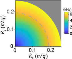
We consider a rigid lossless substrate immersed in air, which has square holes of depth $l$ and side length $w$ forming a two-dimensional square lattice in the $xy$ plane with period $q$ , as depicted in Fig. 1(a). The substrate supports SSWs propagating in the $xy$ -plane [47, 48]. In the deep subwavelength limit ( $\lambda\gg q$ ), the SSWs have an isotropic dispersion $\beta=k_{0}\sqrt{1+\left(w/q\right)^{4}\tan^{2}\left(k_{0}l\right)}$ , where $\beta$ is the propagation constant and $k_{0}=\omega/c$ is wavevector in free space [49]. This analytical dispersion relation is shown in Fig. 1(b) as the solid red line, which agrees with the simulation result (symbols). The simulation results in this paper are obtained with COMSOL Multiphysics.

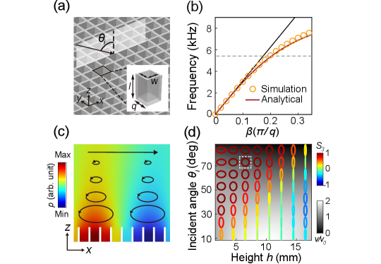
Refer to caption — Figure 1: (a) The substrate drilled with periodic square blind holes. The inset shows the unit cell. (b) Dispersion relation of the SSWs supported by the holey substrate with $w=4.5\mathrm{~{}mm},l=7.5\mathrm{~{}mm}$ and $q=5.5\mathrm{~{}mm}$ . The black solid line denotes the sound dispersion in free space. (c) Velocity polarization ellipses of the SSW. (d) Polarization and normalized amplitude of the background velocity field for different $h$ (the height above the substrate) and incident angles $\theta_{i}$ .

For the SSW propagating in $\pm x$ direction, the velocity field can be expressed as $\mathbf{v}=(v_{x},0,v_{z})=(\pm n_{\mathrm{eff}},0,i\gamma)e^{\pm ik_{0}n_{\mathrm{eff}}x-k_{0}\gamma z}$ , where $n_{\text{eff }}=\beta/k_{0}$ is the effective index, and $\gamma=\sqrt{n_{\text{eff}}^{2}-1}$ characterizes the field’s decay. Since $v_{x}$ and $v_{z}$ have a $\pi/2$ phase difference, the velocity field is elliptically polarized, as depicted in Fig. 1 (c) for the SSW propagating in $+x$ direction at $f=5378\mathrm{~{}Hz}$ (corresponding to the frequency marked by the dashed lines in Fig. 1(b)). Thus, the SSW carries a transverse spin in $-y$ direction. By time-reversal symmetry, the SSW propagating in $-x$ direction carries a transverse spin in $+y$ direction. This locking between the spin direction and propagation direction is known as the spin-momentum locking or transverse spin-orbit interaction [50, 51, 52, 53, 54].

Transverse spin can also appear in the interference of freely propagating waves [45, 55]. We consider a plane wave illuminates the holey substrate with incident angle $\theta_{i}$ in $xz$ plane, as shown in Fig. 1(a). The incident wave will interfere with the reflected wave, giving rise to an inhomogeneous total velocity field $\mathbf{v}$ above the substrate. Figure 1(d) shows the numerically determined polarization ellipses of $\mathbf{v}$ as a function of $h$ (the height above the substrate) and $\theta_{i}$ . The color of the ellipses denotes the Stokes parameter $S_{3}$ characterizing the spin [56]. The background color shows $v/v_{0}$ with $v=|\mathbf{v}|$ and $v_{0}$ being the incident amplitude. Clearly, the polarization and amplitude of $\mathbf{v}$ depend on both $h$ and $\theta_{i}$ . For a fixed $\theta_{i}$ , $S_{3}$ varies with $h$ and can change sign across the interference pattern. Specially, at $\theta_{i}=$ $73^{\circ}$ and $h=6.5\mathrm{~{}mm}$ (marked by the white dashed box) we obtain $S_{3}=1$ , corresponding to circular polarization [49]. Therefore, both the SSWs and the interference wave carry a transverse spin, which is essential to realizing the PB phase.

Meta-atoms with pure dipole response
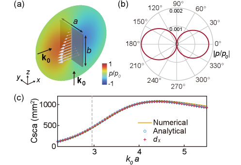
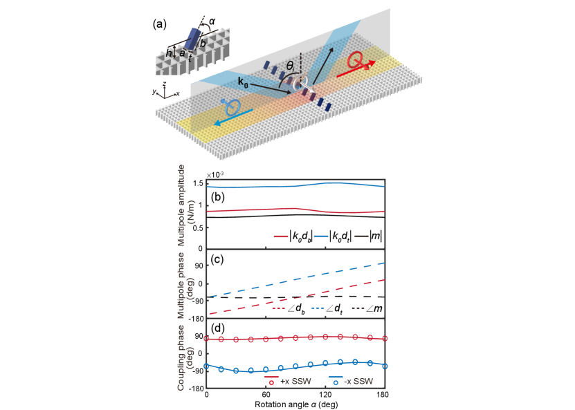
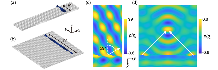
The undesired monopole mode of meta-atoms will contribute to the total field, making the PB phase ambiguous [49]. Thus, it is necessary to design acoustic meta-atoms supporting pure dipole mode. We consider the thin rigid plate in Fig. 2(a) under the incidence of the velocity field $\mathbf{v}=\left(v_{x},0,v_{z}\right)=$ $\frac{p_{0}}{\sqrt{2}\rho_{0}c}\left(e^{ik_{0}x},0,ie^{ik_{0}z}\right)$ . The plate can give rise to an acoustic dipole $\mathbf{d}=\oint\mathbf{D}(\mathbf{r})\mathrm{d}A$ in $x$ direction, where $\mathbf{D}=\mathbf{n}p_{t}$ is the surface dipole density (white arrows) with $\mathbf{n}$ being the surface unit normal vector and $p_{t}$ is surface total pressure (see details in [49]). Figure 2(a) also shows the normalized scattered pressure $p/p_{0}$ on the $xz$ plane in the near field. Figure 2(b) shows $|p/p_{0}|$ in the far field. As noticed, both the near-field and far-field pressure characteristics correspond to a dipole mode. The scattering cross section contributed by the dipole is $C_{\mathrm{sca}}^{\mathbf{d}}=\frac{k_{0}^{2}}{24\pi\rho_{0}cI_{0}}|\mathbf{d}|^{2}$ with $I_{0}$ being the incident intensity [49], which agrees well with the numerically simulated total scattering cross section of the plate, as shown in Fig. 2(c). The cross symbols denote the contribution of the dipole component $d_{x}$ , confirming that the dipole is normal to the plate (along $x$ direction). Therefore, the thin plate can serve as the meta-atom to manipulate the velocity field polarization through its dipole mode. We note that the above property applies to general thin rigid plates satisfying $t\ll a<\lambda$ and $t\ll b<\lambda$ [49].

Acoustic PB geometric phase
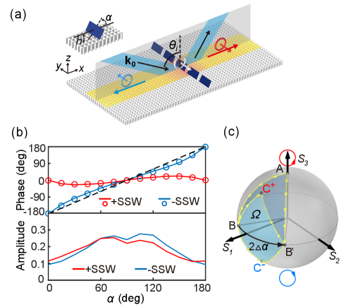
We construct a metasurface by arranging the meta-atoms on the holey substrate periodically along $y$ direction with a period of $p$ , as shown in Fig. 3(a). The orientation of the meta-atoms in $xz$ plane is characterized by the angle $\alpha$ with respect to $x$ axis. A plane wave obliquely incidents in $xz$ plane with angle $\theta_{i}$ . As discussed earlier, the interference of the incident and reflected fields gives rise to a circularly polarized velocity field at the positions of the meta-atoms, as denoted by the white circle with an arrow in Fig. 3(a). This background velocity field excites a linearly polarized acoustic dipole $\mathbf{d}$ in each meta-atom. The fields of $\mathbf{d}$ couple to the SSWs propagating in $+x$ and $-x$ directions, denoted as $+$ SSW and $-$ SSW, respectively. This process is accompanied by the variations of the velocity polarization, which induces the PB geometric phase. We determine the PB phase for different meta-atom rotation angles $\alpha$ by numerically simulating the SSWs’ phase. The results are shown in the upper panel of Fig. 3(b), where the red (blue) solid line denotes the PB phase $\Phi_{\text{PB}}^{+}$ ( $\Phi_{\text{PB}}^{-}$ ) for $+$ SSW ( $-$ SSW). Remarkably, the PB phase exhibits a Janus property: $\Phi_{\text{PB}}^{+}$ and $\Phi_{\text{PB}}^{-}$ have different values. $\Phi_{\text{PB}}^{-}$ can cover $2\pi$ , but $\Phi_{\text{PB}}^{+}$ cannot. We notice that $\Phi_{\text{PB}}^{-}$ slightly deviates from the linear relation $\Phi_{\text{PB}}^{-}=2\alpha$ (dashed line), which is different from the conventional PB phase in optical metasurfaces and is attributed to the elliptical polarization of the SSWs. The elliptical polarization also results in different amplitudes of the SSWs at different $\alpha$ , as shown in the lower panel of Fig. 3(b).

Poincaré sphere interpretation
The acoustic PB geometric phase can be intuitively understood with the Poincaré sphere describing the polarization of vector fields [20, 21]. Figure 3(c) shows the evolutions of velocity polarization on the Poincaré sphere for the system in Fig. 3(a). The polarization of the background velocity field corresponds to the north pole (point A). The velocity polarization of $\pm$ SSW can be characterized by the Stokes vector $\mathbf{S}^{\mathrm{s}}=\left(S_{1}^{\mathrm{s}},S_{2}^{\mathrm{s}},S_{3}^{\mathrm{s}}\right)=\left(\frac{1}{n_{\text{eff }}^{2}+\gamma^{2}},0,\frac{\pm 2\gamma n_{\mathrm{eff}}}{n_{\text{eff }}^{2}+\gamma^{2}}\right)$ , corresponding to the point $\text{C}^{\pm}$ . The acoustic dipole $\mathbf{d}$ of the meta-atom has $\mathbf{S}^{\mathrm{d}}=\left(S_{1}^{d},S_{2}^{d},S_{3}^{d}\right)=$ $[\cos(2\alpha),\sin(2\alpha),0]$ , corresponding to the point B on the equator. A variation of the meta-atom’s rotation angle $(\Delta\alpha)$ changes its polarization from $\mathrm{B}$ to $\mathrm{B}^{\prime}$ . The corresponding change of the PB phase equals half of the solid angle $\Omega$ subtended by the area enclosed by the loop A $\rightarrow\mathrm{B}\rightarrow\mathrm{C}^{\pm}\rightarrow\mathrm{B}^{\prime}\rightarrow\mathrm{A}$ [20, 21, 57]. We evaluate $\Omega$ to obtain the geometric phase. The results are denoted by the blue and red circles in the upper panel of Fig. 3(b), which are consistent with the numerical results (solid blue and red lines) obtained by directly simulating the SSWs’ phase. Notably, the maximum solid angle for $+$ SSW is less than $4\pi$ while it can reach $4\pi$ for $-$ SSW due to the spin flipping [49].

Wavefront manipulation
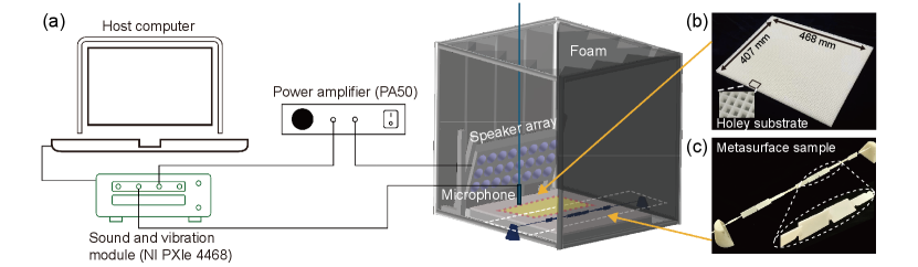
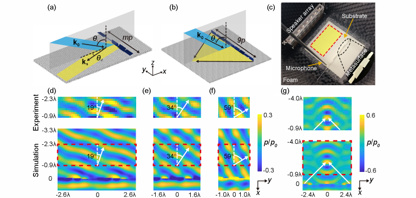
The acoustic PB phase offers a powerful mechanism for nearly arbitrary manipulation of the SSWs’ wavefront. As shown in Figs. 4(a) and 4(b), we design acoustic PB metasurfaces to demonstrate two typical wavefront manipulations, i.e., anomalous deflection and focusing, for $-$ SSW since $\Phi_{\text{PB}}^{-}$ can cover $2\pi$ . We conduct both full-wave simulations and experiments. The experiments are performed in an anechoic room with absorbing foams installed on the walls, as shown in Fig. 4(c). A speaker array is used to generate the incident plane wave, and a microphone mounted on a moving stage is used to measure the pressure field of the SSW (see details in [49]). The substrate and meta-atoms are fabricated by 3D printing.

For the demonstration of anomalous deflection in Fig. 4(a), we design three PB metasurfaces with different phase gradients $k_{g}=\Delta\Phi_{\text{PB}}^{-}/p=2\pi/5p$ , $2\pi/3p$ , and $2\pi/$ $3p$ with $p=33\mathrm{~{}mm},33\mathrm{~{}mm}$ , and $22\mathrm{~{}mm}$ , respectively, and $\Delta\Phi_{\text{PB}}^{-}$ is PB phase difference between two nearby meta-atoms. The SSW will be deflected by angle $\theta_{d}=$ $\sin^{-1}\left(k_{g}/\beta\right)$ by the generalized Snell’s law [58, 59]. The upper panels of Fig. 4(d-f) show the experimentally measured pressure field of the SSW, which agree well with the simulation results in the lower panels (i.e., regions enclosed by the red rectangles). The analytical results of $\theta_{d}$ are indicated by the white arrows, which agree with the simulated and experimentally measured wavefronts.

For the demonstration of focusing in Fig. 4(b), we design a PB metalens with geometric phase profile $\Phi_{\text{PB}}^{-}(y)=-\beta\left(\sqrt{y^{2}-f^{2}}-f\right)$ [58], where $f$ is the focal length and $y$ denotes the location of the meta-atoms. The metalens can convert the incident plane wave to the SSW converging at a desired focal point. Figure 4(g) shows the experimental (upper panel) and simulation (lower panel) results for the SSW’s pressure field, which agree well with each other. We observe the focusing of the SSW with a focal length $f=2.1\lambda$ . The analytically predicted focal length based on the expression of $\Phi_{\text{PB}}^{-}(y)$ is indicated by the white arrows, which is consistent with the experimental and simulation results. These results demonstrate the unprecedented capability of the acoustic PB phase in manipulating the SSWs. The manipulation efficiency can be further enhanced if a continuous design of the metasurface is adopted, i.e., replacing the discrete meta-atoms by a helical ribbon with pitch gradient (see [49]).

Discussion and conclusion
Our results show that the vector degree of freedom in sound waves (i.e., velocity field) can be exploited to achieve wavefront manipulations in a manner similar to the electric or magnetic field in optics, despite its curl-free longitudinal nature. The acoustic spin deriving from circularly polarized velocity fields can induce the acoustic PB phase, which offers a new mechanism for controlling sound waves beyond the limitations of the conventional propagation and resonant phases [58, 60, 61]. There are many other intriguing properties of acoustic spin uncovered in recent literature, including acoustic spin-orbit interactions [45, 46, 62, 63, 64], acoustic spin-induced torque [65, 66], and topological spin textures [67, 68, 69, 70]. These discoveries offer new insights into the fundamental properties of sound waves.

In conclusion, we demonstrate the acoustic PB phase induced by transverse spin, providing the missing piece of acoustic geometric phases. The phase arises in the SSWs interacting with anisotropic meta-atoms. We apply the mechanism to realize acoustic PB metasurfaces for the steering and focusing of the SSWs, demonstrating its vast application potential. The acoustic PB phase can revolutionize sound manipulations, akin to the optical PB phase, which has already revolutionized light manipulations.

Acknowledgements
The work described in this paper was supported by grants from the Research Grants Council of the Hong Kong Special Administrative Region, China (Project No. AoE/P-502/20) and National Natural Science Foundation of China (No. 12322416).

Author contributions
S.W. conceived the idea. W.X. performed the numerical simulations and analytical calculations. W.X., W.K., and S.H. conducted the experiment. W.X., W.K., S.H., S.L., D.P.T., and S.W. analyzed the results. W.X. and S.W. wrote the manuscript with input from all authors. S.L. and S.W. supervised the project.

References

Berry [1984] M. V. Berry, roc. R. Soc. A: Math. Phys. Eng. Sci. 392, 45 (1984).
Gonoskov et al. [2022] A. Gonoskov, T. Blackburn, M. Marklund, and S. Bulanov, Rev. Mod. Phys. 94, 045001 (2022).
Simon [1983] B. Simon, Phys. Rev. Lett. 51, 2167 (1983).
Aharonov and Bohm [1959] Y. Aharonov and D. Bohm, Phys. Rev. 115, 485 (1959).
Thouless et al. [1982] D. J. Thouless, M. Kohmoto, M. P. Nightingale, and M. den Nijs, Phys. Rev. Lett. 49, 405 (1982).
Kane and Mele [2005] C. L. Kane and E. J. Mele, Phys. Rev. Lett. 95, 226801 (2005).
Bernevig et al. [2006] B. A. Bernevig, T. L. Hughes, and S.-C. Zhang, Science 314, 1757 (2006).
Ozawa et al. [2019] T. Ozawa, H. M. Price, A. Amo, N. Goldman, M. Hafezi, L. Lu, M. C. Rechtsman, D. Schuster, J. Simon, O. Zilberberg, and I. Carusotto, Rev. Mod. Phys. 91, 015006 (2019).
Xue et al. [2022] H. Xue, Y. Yang, and B. Zhang, Nat. Rev. Mater. 7, 974 (2022).
Wang et al. [2009] Z. Wang, Y. Chong, J. D. Joannopoulos, and M. Soljačić, Nature 461, 772 (2009).
Yang et al. [2020] Y. Yang, Y. Yamagami, X. Yu, P. Pitchappa, J. Webber, B. Zhang, M. Fujita, T. Nagatsuma, and R. Singh, Nat. Photonics 14, 446 (2020).
Bandres et al. [2018] M. A. Bandres, S. Wittek, G. Harari, M. Parto, J. Ren, M. Segev, D. N. Christodoulides, and M. Khajavikhan, Science 359, eaar4005 (2018).
Yang et al. [2022] L. Yang, G. Li, X. Gao, and L. Lu, Nat. Photonics 16, 279 (2022).
Mittal et al. [2018] S. Mittal, E. A. Goldschmidt, and M. Hafezi, Nature 561, 502 (2018).
Barik et al. [2018] S. Barik, A. Karasahin, C. Flower, T. Cai, H. Miyake, W. DeGottardi, M. Hafezi, and E. Waks, Science 359, 666 (2018).
Chen et al. [2021] Y. Chen, X.-T. He, Y.-J. Cheng, H.-Y. Qiu, L.-T. Feng, M. Zhang, D.-X. Dai, G.-C. Guo, J.-W. Dong, and X.-F. Ren, Phys. Rev. Lett. 126, 230503 (2021).
Rytov [1938] S. Rytov, Dokl. Akad. Nauk SSSR 18, 263 (1938).
Vladimirskii [1941] V. Vladimirskii, Dokl. Akad. Nauk SSSR 21, 1941 (1941).
Chiao and Wu [1986] R. Y. Chiao and Y.-S. Wu, Phys. Rev. Lett. 57, 933 (1986).
Pancharatnam [1956] S. Pancharatnam, Proc. Indian Acad. Sci. 44, 247 (1956).
Berry [1987] M. V. Berry, J. Mod. Opt. 34, 1401 (1987).
Tomita and Chiao [1986] A. Tomita and R. Y. Chiao, Phys. Rev. Lett. 57, 937 (1986).
Bliokh et al. [2008a] K. Y. Bliokh, A. Niv, V. Kleiner, and E. Hasman, Nat. Photonics 2, 748 (2008a).
Onoda et al. [2004] M. Onoda, S. Murakami, and N. Nagaosa, Phys. Rev. Lett. 93, 083901 (2004).
Bliokh et al. [2008b] K. Y. Bliokh, Y. Gorodetski, V. Kleiner, and E. Hasman, Phys. Rev. Lett. 101, 030404 (2008b).
Hosten and Kwiat [2008] O. Hosten and P. Kwiat, Science 319, 787 (2008).
Zhao et al. [2007] Y. Zhao, J. S. Edgar, G. D. Jeffries, D. McGloin, and D. T. Chiu, Phys. Rev. Lett. 99, 073901 (2007).
Rodríguez-Herrera et al. [2010] O. G. Rodríguez-Herrera, D. Lara, K. Y. Bliokh, E. A. Ostrovskaya, and C. Dainty, Phys. Rev. Lett. 104, 253601 (2010).
Bliokh et al. [2011] K. Y. Bliokh, E. A. Ostrovskaya, M. A. Alonso, O. G. Rodríguez-Herrera, D. Lara, and C. Dainty, Opt. Express 19, 26132 (2011).
Bomzon et al. [2002] Z. Bomzon, G. Biener, V. Kleiner, and E. Hasman, Opt. Lett. 27, 1141 (2002).
Marrucci et al. [2006] L. Marrucci, C. Manzo, and D. Paparo, Phys. Rev. Lett. 96, 163905 (2006).
Wang et al. [2018a] S. Wang, P. C. Wu, V.-C. Su, Y.-C. Lai, M.-K. Chen, H. Y. Kuo, B. H. Chen, Y. H. Chen, T.-T. Huang, J.-H. Wang, et al., Nat. Nanotechnol. 13, 227 (2018a).
Chen et al. [2018] W. T. Chen, A. Y. Zhu, V. Sanjeev, M. Khorasaninejad, Z. Shi, E. Lee, and F. Capasso, Nat. Nanotechnol. 13, 220 (2018).
Zheng et al. [2015] G. Zheng, H. Mühlenbernd, M. Kenney, G. Li, T. Zentgraf, and S. Zhang, Nat. Nanotechnol. 10, 308 (2015).
Li et al. [2015a] G. Li, S. Chen, N. Pholchai, B. Reineke, P. W. H. Wong, E. Y. B. Pun, K. W. Cheah, T. Zentgraf, and S. Zhang, Nat. Mater. 14, 607 (2015a).
Peng et al. [2022] J. Peng, R.-Y. Zhang, S. Jia, W. Liu, and S. Wang, Sci. Adv. 8, eabq0910 (2022).
Fu et al. [2024] T. Fu, R.-Y. Zhang, S. Jia, C. T. Chan, and S. Wang, Phys. Rev. Lett. 132, 233801 (2024).
Demore et al. [2012] C. E. Demore, Z. Yang, A. Volovick, S. Cochran, M. P. MacDonald, and G. C. Spalding, Phys. Rev. Lett. 108, 194301 (2012).
Jiang et al. [2016] X. Jiang, Y. Li, B. Liang, J.-c. Cheng, and L. Zhang, Phys. Rev. Lett. 117, 034301 (2016).
Wang et al. [2018b] S. Wang, G. Ma, and C. T. Chan, Sci. Adv. 4, eaaq1475 (2018b).
Liu et al. [2021] B. Liu, Z. Su, Y. Zeng, Y. Wang, L. Huang, and S. Zhang, New J. Phys. 23, 113026 (2021).
Liu et al. [2022] B. Liu, Z. Zhou, Y. Wang, T. Zentgraf, Y. Li, and L. Huang, Appl. Phys. Lett. 120 (2022).
Zhang et al. [2023] K. Zhang, X. Li, D. Dong, M. Xue, W.-L. You, Y. Liu, L. Gao, J.-H. Jiang, H. Chen, Y. Xu, et al., Adv. Sci 10, 2304992 (2023).
Bliokh and Nori [2019a] K. Y. Bliokh and F. Nori, Phys. Rev. B 99, 174310 (2019a).
Shi et al. [2019] C. Shi, R. Zhao, Y. Long, S. Yang, Y. Wang, H. Chen, J. Ren, and X. Zhang, Natl. Sci. Rev. 6, 707 (2019).
Wang et al. [2021] S. Wang, G. Zhang, X. Wang, Q. Tong, J. Li, and G. Ma, Nat. Commun. 12, 6125 (2021).
Liu et al. [2018] T. Liu, S. Liang, F. Chen, and J. Zhu, J. Appl. Phys. 123 (2018).
Liu et al. [2019] T. Liu, F. Chen, S. Liang, H. Gao, and J. Zhu, Phys. Rev. Appl. 11, 034061 (2019).
[49] See Supplemental Material for additional experimental information and discussions about the dispersion relation of the SSWs, transverse spin of background field, multipolar expansions and scattering properties of the meta-atom, effect of monopole mode, etc .
Bliokh and Nori [2015] K. Y. Bliokh and F. Nori, Phys. Rep. 592, 1 (2015).
Bliokh and Nori [2019b] K. Y. Bliokh and F. Nori, Phys. Rev. B 99, 020301 (2019b).
Bliokh et al. [2014] K. Y. Bliokh, A. Y. Bekshaev, and F. Nori, Nat. Commun. 5, 3300 (2014).
Van Mechelen and Jacob [2016] T. Van Mechelen and Z. Jacob, Optica 3, 118 (2016).
Xiao and Wang [2024] W. Xiao and S. Wang, Opt. Lett. 49, 1915 (2024).
Bekshaev et al. [2015] A. Y. Bekshaev, K. Y. Bliokh, and F. Nori, Phys. Rev. X 5, 011039 (2015).
Jackson [2012] J. D. Jackson, Classical electrodynamics (John Wiley & Sons, 2012).
Cohen et al. [2019] E. Cohen, H. Larocque, F. Bouchard, F. Nejadsattari, Y. Gefen, and E. Karimi, Nat. Rev. Phys. 1, 437 (2019).
Li et al. [2014] Y. Li, X. Jiang, R.-q. Li, B. Liang, X.-y. Zou, L.-l. Yin, and J.-c. Cheng, Phys. Rev. Appl. 2, 064002 (2014).
Assouar et al. [2018] B. Assouar, B. Liang, Y. Wu, Y. Li, J.-C. Cheng, and Y. Jing, Nat. Rev. Mater. 3, 460 (2018).
Li et al. [2015b] Y. Li, X. Jiang, B. Liang, J.-c. Cheng, and L. Zhang, Phys. Rev. Appl. 4, 024003 (2015b).
Zhao et al. [2018] S.-D. Zhao, A.-L. Chen, Y.-S. Wang, and C. Zhang, Phys. Rev. Appl. 10, 054066 (2018).
Long et al. [2020a] Y. Long, D. Zhang, C. Yang, J. Ge, H. Chen, and J. Ren, Nat. Commun. 11, 4716 (2020a).
Long et al. [2020b] Y. Long, H. Ge, D. Zhang, X. Xu, J. Ren, M.-H. Lu, M. Bao, H. Chen, and Y.-F. Chen, Natl. Sci. Rev. 7, 1024 (2020b).
Alhaïtz et al. [2023] L. Alhaïtz, T. Brunet, C. Aristégui, O. Poncelet, and D. Baresch, Phys. Rev. Lett. 131, 114001 (2023).
Toftul et al. [2019] I. D. Toftul, K. Y. Bliokh, M. I. Petrov, and F. Nori, Phys. Rev. Lett. 123, 183901 (2019).
Lopes et al. [2020] J. H. Lopes, E. B. Lima, J. P. Leão Neto, and G. T. Silva, Phys. Rev. E 101, 043102 (2020).
Bliokh et al. [2021] K. Y. Bliokh, M. A. Alonso, D. Sugic, M. Perrin, F. Nori, and E. Brasselet, Phys. Fluids 33 (2021).
Ge et al. [2021] H. Ge, X.-Y. Xu, L. Liu, R. Xu, Z.-K. Lin, S.-Y. Yu, M. Bao, J.-H. Jiang, M.-H. Lu, and Y.-F. Chen, Phys. Rev. Lett. 127, 144502 (2021).
Muelas-Hurtado et al. [2022] R. D. Muelas-Hurtado, K. Volke-Sepúlveda, J. L. Ealo, F. Nori, M. A. Alonso, K. Y. Bliokh, and E. Brasselet, Phys. Rev. Lett. 129, 204301 (2022).
Tong and Wang [2023] Q. Tong and S. Wang, arXiv preprint 2312.12283 (2023).
Howe [2003] M. S. Howe, Theory of Vortex Sound, 33 (Cambridge University Press, 2003).
Morse and Ingard [1986] P. M. Morse and K. U. Ingard, Theoretical Acoustics (Princeton university press, 1986).
Wrobel [2002] L. C. Wrobel, The Boundary Element Method, Vol. 1 (John Wiley & Sons, 2002).
Alaee et al. [2018] R. Alaee, C. Rockstuhl, and I. Fernandez-Corbaton, Opt. Commun. 407, 17 (2018).
Boström [1991] A. Boström, J. Acoust. Soc. Am. 90, 3344 (1991).

Supplemental Materials for
Acoustic Pancharatnam-Berry Geometric Phase Induced by Transverse Spin

NOTE 1. Dispersion relation of the SSWs

We consider the holey substrate shown in Fig. 1(a) of the main text. The reflection coefficient of the substrate can be expressed as [47]

R_{mn}=\delta_{mn,00}-\frac{2i\tan\left(k_{0}l\right)\frac{w^{2}}{q^{2}}\xi_{00}\xi_{mn}\frac{k_{0}}{k_{z}^{(m,n)}}}{1+i\tan\left(k_{0}l\right)\frac{w^{2}}{q^{2}}\sum_{r,s=-\infty}^{+\infty}\frac{k_{0}}{k_{z}^{(r,s)}}\xi_{rs}^{2}}.

Here $\xi_{mn}=\operatorname{sinc}\left(k_{x}^{(m)}q/2\right)\operatorname{sinc}\left(k_{y}^{(n)}q/2\right)$ with $k_{x}^{(m)}=k_{x}+\frac{2\pi m}{q},k_{y}^{(n)}=k_{y}+\frac{2\pi n}{q}$ and $k_{z}^{(m,n)}=\sqrt{k_{0}^{2}-\left(k_{x}^{(m)}\right)^{2}-\left(k_{y}^{(n)}\right)^{2}}$ , where $k_{x}$ and $k_{y}$ are the $x$ and $y$ components of the incident wave vector, respectively, and $m,n,r$ , and $s$ are integers. The dispersion relation of the SSWs can be obtained by analyzing the poles of the reflection coefficient in Eq. (S1) [47]

1-k_{0}\tan\left(k_{0}l\right)\frac{w^{2}}{q^{2}}\sum_{m,n=-\infty}^{+\infty}\frac{\xi_{mn}^{2}}{\sqrt{\left(\beta^{(m,n)}\right)^{2}-k_{0}^{2}}}=0.

Here $\beta^{(m,n)}=\sqrt{\left(k_{x}^{(m)}\right)^{2}+\left(k_{y}^{(n)}\right)^{2}}$ is the propagation constant of the SSWs. For the SSW propagating in $x$ direction with $m=n=0$ , we can obtain

1-\tan\left(k_{0}l\right)\frac{w^{2}}{q^{2}}\frac{\operatorname{sinc}^{2}\left(\frac{\beta a}{2}\right)}{\sqrt{\frac{\beta^{2}}{k_{0}^{2}}-1}}=0,

where $\beta=\beta^{(0,0)}=k_{x}^{(0)}$ . In the deep subwavelength limit $q\ll\lambda$ , $\operatorname{sinc}(\beta a/2)\approx 1$ , Eq. (S3) is reduced to an isotropic dispersion relation

\beta=k_{0}\sqrt{1+\left(\frac{w}{q}\right)^{4}\tan^{2}\left(k_{0}l\right)}.

This is the dispersion relation shown in Fig. 1 (b) of the main text. Figure S1 shows the simulated isofrequency contours of the dispersion relation. Clearly, the holey substrate is effectively homogeneous and isotropic for the SSWs in the considered frequency range.

NOTE 2. Transverse spin due to the interference of the incident and reflected waves

We consider the holey substrate under the incidence of a plane wave propagating in $xz$ plane with the incident angle $\theta_{i}$ . If $q\ll\lambda$ , $\operatorname{sinc}(\beta a/2)\approx 1$ , Eq. (S1) is reduced to

R=\frac{1-i\tan\left(k_{0}l\right)\frac{w^{2}}{q^{2}}\frac{1}{\cos\left(\theta_{i}\right)}}{1+i\tan\left(k_{0}l\right)\frac{w^{2}}{q^{2}}\frac{1}{\cos\left(\theta_{i}\right)}}=e^{i\phi}.

Here $\phi=\operatorname{acos}\frac{1-\left[\tan\left(k_{0}l\right)\frac{w^{2}}{q^{2}\cos\left(\theta_{i}\right)}\right]^{2}}{1+\left[\tan\left(k_{0}l\right)\frac{w^{2}}{q^{2}\cos\left(\theta_{i}\right)}\right]^{2}}$ is the reflective phase shift at the substrate surface. The incident wave interferes with the reflected wave, giving rise to an inhomogeneous total velocity field above the substrate. The two components $v_{x}$ and $v_{z}$ of the total velocity field satisfy

\frac{v_{x}}{v_{z}}=\tan\left(\theta_{i}\right)\frac{1+e^{2ik_{0}\cos\left(\theta_{i}\right)h}R}{1-e^{2ik_{0}\cos\left(\theta_{i}\right)h}R},

(1)

where $h$ is the height above the substrate. Substitute Eq. (S5) into Eq. (S6), we can obtain

\frac{v_{x}}{v_{z}}=\frac{\tan\left(\theta_{i}\right)}{\tan\left(\frac{\psi}{2}\right)}e^{\pm i\frac{\pi}{2}},

(2)

and the $S_{3}$ parameter can be obtained as

S_{3}=\frac{\mp 2\tan\left(\theta_{i}\right)\tan\left(\frac{\psi}{2}\right)}{\tan^{2}\left(\theta_{i}\right)+\tan^{2}\left(\frac{\psi}{2}\right)},

(3)

where $\psi=2k_{0}\cos\left(\theta_{i}\right)h+\phi$ $(\psi\in[0,2\pi])$ , and the sign ’ $+$ ’ (’ $-$ ’) is for $\psi>\pi$ $(\psi<\pi)$ . Clearly, the polarization of the total velocity field depends on the incident angle $\theta_{i}$ and the spatial position above the substrate (i.e., $h$ ). For a fixed incident angle, the $S_{3}$ parameter varies with $h$ and can change sign across the interference pattern. Specially, we obtain $S_{3}=1$ for $\theta_{i}=73^{\circ}$ and $h=6.5\mathrm{~{}mm}$ .

NOTE 3. Multipole expansion of the meta-atom scattering field

The linear acoustic wave equation with generic sources can be written as [71]

	$\displaystyle\frac{1}{c^{2}\rho_{0}}\frac{\partial p(\mathbf{r},t)}{\partial t}+\nabla\cdot\mathbf{v}(\mathbf{r},t)=q(\mathbf{r},t),$		(S9)
	$\displaystyle\rho_{0}\frac{\partial\mathbf{v}(\mathbf{r},t)}{\partial t}+\nabla p(\mathbf{r},t)=\mathbf{F}(\mathbf{r},t),$		(S10)

where $q(\mathbf{r},t)$ is volume change rate which can be related to monopole density by $M(\mathbf{r},t)=$ $\rho_{0}\frac{\partial q(\mathbf{r},t)}{\partial t},\mathbf{F}(\mathbf{r},t)$ is the force density which can be defined as the dipole density $\mathbf{D}(\mathbf{r},t)=\mathbf{F}(\mathbf{r},t)$ . Equations (S9) and (S10) correspond to the conservation law of mass and the conservation law of momentum, respectively. Based on the two equations, we can obtain the inhomogeneous Helmholtz wave equation for the monochromatic time-harmonic acoustic wave of frequency $\omega$ :

\left(\nabla^{2}+k_{0}^{2}\right)p(\mathbf{r})=\nabla\cdot\mathbf{D}(\mathbf{r})-M(\mathbf{r}).

The corresponding Green’s function $G\left(\mathbf{r},\mathbf{r}^{\prime}\right)$ is

\left(\nabla^{2}+k_{0}^{2}\right)G\left(\mathbf{r},\mathbf{r}^{\prime}\right)=-\delta\left(\mathbf{r}-\mathbf{r}^{\prime}\right),

and the general solution satisfying radiation boundary condition is $G\left(\mathbf{r},\mathbf{r}^{\prime}\right)=\frac{e^{ik_{0}\left|\mathbf{r}-\mathbf{r}^{\prime}\right|}}{4\pi|\mathbf{r}-\mathbf{r}{\prime}|}$ . The pressure field outside the source volume $\tau$ can be obtained by using the Green’s function [72]

p(\mathbf{r})=-\int_{\tau}\nabla\cdot\mathbf{D}\left(\mathbf{r}^{\prime}\right)G\left(\mathbf{r},\mathbf{r}^{\prime}\right)d^{3}r^{\prime}+\int_{\tau}M\left(\mathbf{r}^{\prime}\right)G\left(\mathbf{r},\mathbf{r}^{\prime}\right)d^{3}r^{\prime}

=\int_{\tau}\mathbf{D}\left(\mathbf{r}^{\prime}\right)\cdot\nabla^{\prime}G\left(\mathbf{r},\mathbf{r}^{\prime}\right)d^{3}r^{\prime}+\int_{\tau}M\left(\mathbf{r}^{\prime}\right)G\left(\mathbf{r},\mathbf{r}^{\prime}\right)d^{3}r^{\prime}.

If the sources only distribute on the boundary of the scatterer, the above equation reduces to

p(\mathbf{r})=\int_{\partial\tau}\mathbf{D}\left(\mathbf{r}^{\prime}\right)\cdot\nabla^{\prime}G\left(\mathbf{r},\mathbf{r}^{\prime}\right)d^{2}r^{\prime}+\int_{\partial\tau}M\left(\mathbf{r}^{\prime}\right)G\left(\mathbf{r},\mathbf{r}^{\prime}\right)d^{2}r^{\prime},

where $\mathbf{D}\left(\mathbf{r}^{\prime}\right)$ and $M\left(\mathbf{r}^{\prime}\right)$ now represent surface densities of the sources. According to the boundary element method [73], the pressure field can be expressed as

p(\mathbf{r})=\int_{\partial\tau}\left[p\left(\mathbf{r}^{\prime}\right)\mathbf{n}\cdot\nabla^{\prime}G\left(\mathbf{r},\mathbf{r}^{\prime}\right)-G\left(\mathbf{r},\mathbf{r}^{\prime}\right)\mathbf{n}\cdot\nabla^{\prime}p\left(\mathbf{r}^{\prime}\right)\right]d^{2}r^{\prime},

where $\mathbf{n}$ is the unit normal vector on the boundary $\partial\tau;$ $p\left(\mathbf{r}^{\prime}\right)\mathbf{n}$ and $-\mathbf{n}\cdot\nabla^{\prime}p\left(\mathbf{r}^{\prime}\right)$ are the boundary source densities. Compare Eq. (S14) with Eq. ( $\mathrm{S}13^{\prime}$ ), we find that $p\left(\mathbf{r}^{\prime}\right)\mathbf{n}$ and $-\mathbf{n}\cdot\nabla^{\prime}p\left(\mathbf{r}^{\prime}\right)$ correspond to the monopole source density and dipole source density, respectively. For a Neumann-type boundary condition $\mathbf{n}\cdot\nabla p=0$ (corresponding to a hard boundary), the normal component of the velocity field is zero $v_{n}\propto\mathbf{n}\cdot\nabla p=0$ , and only the dipole source density $\mathbf{D}\left(\mathbf{r}^{\prime}\right)=p\left(\mathbf{r}^{\prime}\right)\mathbf{n}$ exists on the boundary. For a Dirichlet-type boundary condition $p=0$ (corresponding to a soft boundary), the pressure field is zero, and only the monopole source $M\left(\mathbf{r}^{\prime}\right)=-\mathbf{n}\cdot\nabla^{\prime}p\left(\mathbf{r}^{\prime}\right)$ exists on the boundary.

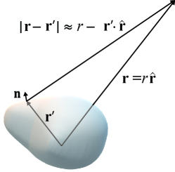
For a rigid scatterer under the incidence of external sound waves, as shown in Fig. S2, only dipole density can be induced on the surface with $\mathbf{D}=\mathbf{n}p_{t}$ , where $p_{t}$ is surface total pressure. Thus, the pressure field in Eq. ( $\mathrm{S}13^{\prime}$ ) reduces to

p(\mathbf{r})=\int_{\partial\tau}\mathbf{D}\left(\mathbf{r}^{\prime}\right)\cdot\nabla^{\prime}G\left(\mathbf{r},\mathbf{r}^{\prime}\right)d^{2}r^{\prime},

Equivalently,

p(\mathbf{r})=\int_{\partial\tau}\mathbf{D}\left(\mathbf{r}^{\prime}\right)\cdot\left[\frac{\mathbf{R}}{R}\left(-ik_{0}+\frac{1}{R}\right)G\left(\mathbf{r},\mathbf{r}^{\prime}\right)\right]d^{2}r^{\prime},

where $R=\left|\mathbf{r}-\mathbf{r}^{\prime}\right|$ . Using the approximation $\left|\mathbf{r}-\mathbf{r}^{\prime}\right|\approx r-\mathbf{r}^{\prime}\cdot\hat{\mathbf{r}}$ with $\hat{\mathbf{r}}=\mathbf{r}/r$ , the scattering far field of a subwavelength scatterer can be expanded as

p(\mathbf{r})=\frac{-ik_{0}}{4\pi}\frac{e^{\mathrm{i}k_{0}r}}{r}\sum_{n}\frac{\left(-\mathrm{i}k_{0}\right)^{n}}{n!}\int_{\partial\tau}\left[\mathbf{D}\left(\mathbf{r}^{\prime}\right)\cdot\hat{\mathbf{r}}\right]\left(\mathbf{r}^{\prime}\cdot\hat{\mathbf{r}}\right)^{n}d^{2}r^{\prime},

The contribution from the first term is

p(\mathbf{r})=\frac{-ik_{0}}{4\pi}\frac{e^{\mathbf{i}k_{0}r}}{r}\hat{\mathbf{r}}\cdot\int_{\partial\tau}\mathbf{D}\left(\mathbf{r}^{\prime}\right)d^{2}r^{\prime},

which corresponds to the far field of an acoustic dipole [72]

p(\mathbf{r})=\frac{-ik_{0}}{4\pi}\frac{e^{\mathrm{i}k_{0}r}}{r}\hat{\mathbf{r}}\cdot\mathbf{d},

with the dipole moment

\mathbf{d}=\int_{\partial\tau}\mathbf{D}\left(\mathbf{r}^{\prime}\right)d^{2}r^{\prime}.

The contribution from the second term in Eq. (S17) is

p(\mathbf{r})=\frac{-ik_{0}}{4\pi}\frac{e^{ik_{0}r}}{r}\left(-ik_{0}\right)\int_{\partial\tau}\left[\mathbf{D}\left(\mathbf{r}^{\prime}\right)\cdot\hat{\mathbf{r}}\right]\left(\mathbf{r}^{\prime}\cdot\hat{\mathbf{r}}\right)d^{2}r^{\prime},

which can be rewritten as

p(\mathbf{r})=\frac{-k_{0}^{2}}{4\pi}\frac{e^{\mathrm{i}k_{0}r}}{r}\hat{\mathbf{r}}\left\{\int_{\partial\tau}\mathbf{D}\left(\mathbf{r}^{\prime}\right)\otimes\mathbf{r}^{\prime}d^{2}r^{\prime}\right\}\hat{\mathbf{r}}^{\mathrm{T}}.

Denote the tensor inside the bracket as $\overline{\mathbf{M}}$ :

\overline{\mathbf{M}}=\int_{\partial\tau}\mathbf{D}\left(\mathbf{r}^{\prime}\right)\otimes\mathbf{r}^{\prime}d^{2}r^{\prime}=\left(\begin{array}[]{lll}M_{xx}&M_{xy}&M_{xz}\\ M_{yx}&M_{yy}&M_{yz}\\ M_{zx}&M_{zy}&M_{zz}\end{array}\right).\

For $\overline{\mathbf{M}}$ with elements $M_{xx}=M_{yy}=M_{zz}\neq 0$ and other elements being zero, Eq. (S22) is reduced to

p(\mathbf{r})=\frac{-k_{0}^{2}}{4\pi}\frac{e^{\mathrm{i}k_{0}r}}{r}\frac{1}{3}\int_{\partial\tau}\mathbf{D}\left(\mathbf{r}^{\prime}\right)\cdot\mathbf{r}^{\prime}d^{2}r^{\prime},

which takes the form of an acoustic monopole [72]

p(\mathbf{r})=m\frac{e^{\mathrm{i}k_{0}r}}{4\pi r}

with amplitude

m=\frac{-k_{0}^{2}}{3}\int_{\partial\tau}\mathbf{D}\left(\mathbf{r}^{\prime}\right)\cdot\mathbf{r}^{\prime}d^{2}r^{\prime}.

For $\overline{\mathbf{M}}$ with other matrix values, it corresponds to an acoustic quadrupole, which usually has much smaller contribution compared to that of monopole and dipole in the deep subwavelength regime.

The expressions of monopole and dipole given by Eq. (S20) and (S26) only apply to the scatterers with geometric dimensions much smaller than the wavelength (i.e., in the deep subwavelength regime). For large scatterers or high frequencies, correction factors have to be introduced to obtain accurate multipoles [74], in which case the monopole and dipole can be determined as

	$\displaystyle m=\frac{-k_{0}^{2}}{3}\int_{\partial\tau}\mathbf{D}\left(\mathbf{r}^{\prime}\right)\cdot\mathbf{r}^{\prime}\frac{3j_{1}\left(k_{0}r^{\prime}\right)}{k_{0}r^{\prime}}d^{2}r^{\prime},$		(S27)
	$\displaystyle\mathbf{d}=\int_{\partial\tau}\mathbf{D}\left(\mathbf{r}^{\prime}\right)\frac{3j_{1}\left(k_{0}r^{\prime}\right)}{k_{0}r^{\prime}}d^{2}r^{\prime},$		(S28)

where $j_{1}\left(k_{0}r^{\prime}\right)$ is the spherical Bessel function.

NOTE 4. Scattering cross sections of the multipoles

The pressure far field of a monopole is given by Eq. (S25). The corresponding velocity far field in radial direction is

v_{r}=\frac{m}{\rho_{0}c}\frac{e^{ik_{0}r}}{4\pi r}.

The time-averaged intensity in the far field reads

I_{r}=\frac{1}{2}\operatorname{Re}\left(pv_{r}^{*}\right)=\frac{m^{2}}{32\pi^{2}r^{2}\rho_{0}c}.

The radiation power is

P=\oint I_{r}r^{2}d\Omega=\frac{m^{2}}{8\pi\rho_{0}c}.

Thus, the scattering cross section due to monopole is

C_{\mathrm{sca}}^{m}=\frac{P}{I_{0}}=\frac{m^{2}}{8\pi\rho_{0}cI_{0}},

where $I_{0}$ is the intensity of the incident wave.

For an acoustic dipole, the pressure far field is given by Eq. (S19). The velocity far field can be written as

v_{r}=\frac{-ik_{0}}{\rho_{0}c}\frac{e^{ik_{0}r}}{4\pi r}\hat{\mathbf{r}}\cdot\mathbf{d}=\frac{-ik_{0}}{\rho_{0}c}\frac{e^{ik_{0}r}}{4\pi r}\left(d_{x}\sin\theta\cos\varphi+d_{y}\sin\theta\sin\varphi+d_{z}\cos\varphi\right).

The scattering cross section due to the dipole can be obtained as in the monopole case:

C_{\mathrm{sca}}^{\mathbf{d}}=\frac{k_{0}^{2}}{24\pi\rho_{0}cI_{0}}|\mathbf{d}|^{2}.

NOTE 5. Scattering properties of the thin plate

We will show that the rigid thin plate can be safely used as a meta-atom to support pure dipole mode as long as its thickness $(t)$ is much smaller than the side lengths $(a,b)$ and the side length is not too large compared with the wavelength. We first consider a rigid plate with negligible thickness $(t\rightarrow 0$ ) and discuss its scattered far field as a function of side lengths $a$ and $b$ , then we explore the influence of the thickness $t$ .

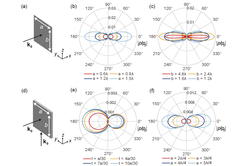
Figure S3(a) shows a rigid plate with a negligible thickness. We assume $a=b$ , and the area of the plate is $a^{2}$ . Under the incidence of a plane wave propagating along $+x$ direction, the scattered pressure amplitude (normalized by the incident pressure amplitude $p_{0}$ ) in the far field (at a distance of $100\lambda$ away from the plate’s center and on the $xz$ -mirror plane) is obtained for different area $a^{2}$ based on the analytical expression given in Ref. [75]. The results are shown in Fig. S3(b). Generally, for a subwavelength plate, its scattered field pattern corresponds to a pure dipole mode. Then, we fix the area of the plate to be $a\times b=(1.2\lambda)^{2}$ and change $b$ from $1.2\lambda$ to $4.8\lambda$ . The calculated farfield pressure amplitude on the $xz$ -mirror plane is shown in Fig. S3(c). Obviously, higher order modes will be excited if $b$ is much larger than the wavelength. Thus, a rigid plate with negligible thickness can support pure dipole mode as long as its side lengths satisfy $a<\lambda$ and $b<\lambda$ .

Figure S3(d) shows a rigid plate with a finite thickness $t$ and side lengths $a=b=\lambda/2$ . Under the incidence of a circularly polarized velocity field $\mathbf{v}=\left(v_{x},0,v_{z}\right)=\frac{p_{0}}{\sqrt{2}\rho_{0}c}\left(e^{ik_{0}x},0,ie^{ik_{0}z}\right)$ , we numerically simulate the scattered pressure amplitude in the far field (on $xz$ -mirror plane) for different thickness $t$ . The results are shown in Fig. S3(e). As seen, the scattered field pattern shows a dipole mode when $t\ll a$ . As $t$ increases, asymmetric scattered field pattern will appear due to the interference of dipole and monopole. The results in Fig. S3(e) indicate that $t=a/30$ is a safe value for exciting pure dipole mode. Figure S3(f) shows the field pattern for different side length $a$ and $t=a/30$ , confirming pure dipole mode is indeed excited.

To summarize, a general rigid thin plate can be used as a meta-atom that support pure dipole mode as long as $t\ll a<\lambda$ and $t\ll b<\lambda$ .

NOTE 6. Effect of monopole on the PB geometric phase

We study the effect of monopole induced in the meta-atom on the PB geometric phase. Let us consider a meta-atom plate with dimensions $a\times b\times t=5.3\mathrm{~{}mm}\times 10.7\mathrm{~{}mm}\times 5.3\mathrm{~{}mm}$ , as shown in the inset of Fig. S4(a), which will induce monopole in addition to dipole according to the above discussions. We arrange the meta-atoms on the substrate (at $h=6.5\mathrm{~{}mm}$ ) periodically along the $y$ direction with a period of $p=16.5\mathrm{~{}mm}$ $(\sim\lambda/4)$ . The incident acoustic plane wave propagate in the $xz$ -plane with the incident angle $\theta_{i}=73^{\circ}$ and frequency $f=5378\mathrm{~{}Hz}$ . Under the excitation of the background circularly polarized field (i.e., the total field due to the interference of the incident and reflected waves), the meta-atom gives rise to two dipole components $d_{t}$ (in the direction along the side $t$ ) and $d_{b}$ (in the direction along the side $b$ ), and a monopole moment $m$ . Figures S4(b) and S4(c) show the amplitude and phase of the excited multipoles as a function of the rotation angle $\alpha$ of the meta-atom, respectively, calculated by using Eqs. (S20) and (S26). We see that the dipole is generally elliptically polarized, and its direction rotates with the meta-atom. Figure S4(d) shows the simulated phases of the SSWs propagating in $+x$ and $-x$ directions. Clearly, the phases cannot cover $2\pi$ , which is different from the cases discussed in the main text. This is attributed to the monopole excited in the meta-atom, which can be understood with coupled mode theory [63].

The eigen fields of the SSWs can be expressed as

\mathbf{F}=\left(v_{x},v_{z},p\right)=\left(\pm n_{\mathrm{eff}},i\gamma,-i\right),

where ’ $+$ ’ (’ $-$ ’) is for the SSW propagating in the $+x$ $(-x)$ direction. The source multipoles induced in the meta-atom can be expressed as

\mathbf{S}=\left(k_{0}d_{x},k_{0}d_{z},m\right).

The coupling coefficient between the multipoles and the SSWs can be determined as

C=\mathbf{F}^{*}\mathbf{S}^{\mathrm{T}},

where ‘ $*$ ’ denotes complex conjugate and ‘T’ denotes tranpose. Using the numerically determined eigen fields of the SSWs and the multipole moments in Figs. S4(b) and S4(c), we determined the coupling phase arg( $C$ ) with Eq. (S37). The results are shown in Fig. S4(d) by the circles, which have good consistency with the simulation results and demonstrating the validity of the coupled mode theory.

We can apply the coupled mode theory to understand the contribution of the monopole to the phase of the SSWs. We decompose Eq. (S37) into a monopole term and dipole term

C=\mathbf{F}^{*}\mathbf{S}^{\mathrm{T}}=\left(\mathbf{F}_{\mathbf{v}}\right)^{*}\left(\mathbf{S}_{\mathbf{v}}\right)^{\mathrm{T}}+im,

where $\mathbf{F}_{\mathbf{v}}=\left(\pm n_{\mathrm{eff}},i\gamma\right)$ and $\mathbf{S}_{\mathbf{v}}=\left(k_{0}d_{x},k_{0}d_{y}\right)=\left(k_{0}d_{b},k_{0}d_{t}\right)\widehat{\mathbb{R}}(-\alpha)$ with $\widehat{\mathbb{R}}(-\alpha)=$ $\left(\begin{array}[]{cc}\cos\alpha&\sin\alpha\\ -\sin\alpha&\cos\alpha\end{array}\right)$ being the rotation matrix and $\left(k_{0}d_{b},k_{0}d_{t}\right)$ being the dipole in the local frame of the meta-atom. The dipole is induced by the background fields and can be expressed as:

\left(k_{0}d_{b},k_{0}d_{t}\right)=\mathbf{S}_{\mathbf{v}}^{\mathrm{e}}\left\{\left[\mathbf{S}_{\mathbf{v}}^{\mathrm{e}}\widehat{\mathbb{R}}(-\alpha)\right]^{*}\left(\mathbf{F}_{\mathbf{v}}^{\mathbf{0}}\right)^{\mathrm{T}}\right\}=\mathbf{S}_{\mathbf{v}}^{\mathrm{e}}\left[\left(\mathbf{S}_{\mathbf{v}}^{\mathrm{e}}\right)^{*}\mathbb{\mathbb{R}}(-\alpha)\left(\mathbf{F}_{\mathbf{v}}^{0}\right)^{\mathrm{T}}\right],

where $\mathbf{S}_{\mathrm{v}}^{\mathrm{e}}$ is the eigen dipole mode of the meta-atom with rotation angle $\alpha=0$ and $\mathbf{F}_{\mathbf{v}}^{0}$ is the background velocity field (i.e., the interference field). Substituting it into Eq. (S38), we obtain

	$\displaystyle C=\left(\mathbf{F}_{\mathbf{v}}\right)^{}\left\{\mathbf{S}_{\mathbf{v}}^{\mathbf{e}}\widehat{\mathbb{R}}(-\alpha)\left[\left(\mathbf{S}_{\mathbf{v}}^{\mathbf{e}}\right)^{}\widehat{\mathbb{R}}(-\alpha)\left(\mathbf{F}_{\mathbf{v}}^{0}\right)^{\mathrm{T}}\right]\right\}^{\mathbf{T}}+im$
	$\displaystyle={\color[rgb]{0,0,1}\left\{\left(\mathbf{F}_{\mathbf{v}}\right)^{}\widehat{\mathbb{R}}(\alpha)\left(\mathbf{S}_{\mathbf{v}}^{\mathrm{e}}\right)^{\mathrm{T}}\right\}}{\color[rgb]{1,0,0}\left\{\left[\left(\mathbf{S}_{\mathbf{v}}^{\mathbf{e}}\right)^{}\widehat{\mathbb{R}}(-\alpha)\right]\left(\mathbf{F}_{\mathbf{v}}^{0}\right)^{\mathrm{T}}\right\}}+im.$		(S40)

Here, the red part characterizes the coupling between the background field and the meta-atom, and the blue part characterizes the coupling between the meta-atom and the SSWs. Apparently, the rotation of the meta-atom only affects the dipole term in the coupling coefficient, it does not affect the monopole term due to the isotropy of the monopole fields. In other words, the PB geometric phase can only manifest in the dipole term. The monopole term will interfere with the dipole term and contribute to the phase of the total field, which makes the PB phase ambiguous.

NOTE 7. The maximum solid angle for the SSWs

The geometric phase for the acoustic PB metasurface in Fig. 3 of main text can be obtained by calculating the solid angle $\Omega$ subtended by the area enclosed by the loop A $\rightarrow\mathrm{B}\rightarrow\mathrm{C}^{\pm}\rightarrow\mathrm{B}^{\prime}\rightarrow\mathrm{A}$ . Figure. S5 (a) and (b) show the maximum solid angles that can be achieved for the $+\mathrm{SSW}$ and $-\mathrm{SSW}$ , respectively. As seen, the maximum solid angle for $+\mathrm{SSW}$ is less than $4\pi$ while it can reach $4\pi$ for $-\mathrm{SSW}$ . This is because that spinning flipping happens when the incident wave is converted to $-\mathrm{SSW}$ by by the metasurface. In contrast, no spin flipping happens for $+\mathrm{SSW}$ .

NOTE 8. PB metasurfaces with helical meta-atoms

The manipulation efficiency of the metasurfaces can be further enhanced if a continuous design of the meta-atoms is adopted, in which case the array of discrete meta-atoms is replaced by a helical ribbon, as shown in Fig. S6(a) for one period of the metasurface. To demonstrate the anomalous deflection of the SSW, the metasurface is designed to exhibit a phase profile $\varphi(y)=k_{g}y$ , where $k_{g}=2\pi/P$ ( $P$ is the period) is the phase gradient. In this case, the helical ribbon can be described by a parametric surface with Cartesian coordinates $x=r\sin(\alpha),z=r\cos(\alpha),y=g(\alpha)$ , where $r\in[-b/2$ , $b/2]$ ( $b$ is the side length of the thin plate in the main text); $\alpha$ is the rotation angle of the helical ribbon in $xz$ plane and $g(\alpha)$ is a function of $\alpha$ . The cross sections of the helical ribbon in different $xz$ cutting planes have different rotation angles $\alpha$ , leading to the $y$ dependent geometric phase $\Phi_{\mathrm{PB}}^{-}(\alpha)=\varphi(y)=k_{g}y$ . Thus, we obtain $g(\alpha)=y=\Phi_{\mathrm{PB}}^{-}(\alpha)/k_{g}$ . The geometric phase $\Phi_{\mathrm{PB}}^{-}(\alpha)$ has been given in Fig. 3(b) of the main text. By setting the parametric equation for the helical ribbon, different phase gradients can be designed to achieve the anomalous deflection of the SSW.

We consider helical ribbon with thickness $t=1\mathrm{~{}mm}$ and width $b=12.5\mathrm{~{}mm}$ , and set $k_{g}=2\pi/P$ with $P=66\mathrm{~{}mm}$ . The phase gradient is equal to that of the metasurface shown in Fig. 4(f) of the main text. Under the incidence of the same plane wave as in Fig. 4, the SSW is deflected by the angle $\theta_{d}=\sin^{-1}\left(k_{g}/\beta\right)=59^{\circ}$ , the simulation results for the pressure field above the substrate is shown in Fig. S6(c). As noticed, the manipulation efficiency of the metasurfaces is enhanced. The deflected SSW has a larger amplitude $p/p_{0}=0.6$ compared to $p/p_{0}=0.3$ of the metasurfaces in Fig. 4. This indicates that the near-field coupling between the discrete acoustic meta-atoms does not affect the performance of the acoustic PB metasurface, in contrast to the optical PB metasurfaces. We note that the PB metasurfaces in the main text allows free adjustment of the rotating angle of each meta-atom and thus can be applied to different scenarios, while the functionality of the metasurface in Fig. S6 is fixed after fabrication.

To demonstrate the focusing of the SSW, we design a metalens using the helical ribbon with a phase profile $\varphi(y)=-\beta\left(\sqrt{y^{2}+f^{2}}-f\right)$ . Figure S6(b) shows the schematic of the metalens. The length of the ribbon is $W$ . From $\varphi(y)=\Phi_{\mathrm{PB}}^{-}(\alpha)$ and $y=g(\alpha)$ , we obtain $g(\alpha)=\pm\sqrt{\left(-\Phi_{\mathrm{PB}}^{-}(\alpha)/\beta+f\right)^{2}-f^{2}}$ , where the sign ’ $+$ ’(’ $-$ ’) is for $y>0$ $(y<0)$ . By setting the parametric equation of the helical ribbon, different focal length can be designed to achieve the focusing of the SSW. We design the metalens with $f=2.1\lambda$ , $d=$ $12.5\mathrm{~{}mm}$ and $W=297\mathrm{~{}mm}$ , which has the same functionality as the metalens in Fig. 4(g) of the main text. The metalens can convert the incident plane wave to the SSW that converges at a desired focal point. Figure S6 (d) shows the simulated pressure field of the SSW in the $xy$ plane. We notice that the performance of the metalens is also improved, i.e., the SSW has a larger amplitude.

NOTE 9. Experimental setup and measurements

The experiments are conducted in a custom low-reflection environment $(0.6\mathrm{~{}m}\times 0.52\mathrm{~{}m}\times 0.6\mathrm{~{}m}$ ) coated by sound-absorbing foams. The schematic of the experiment setup is shown in Fig. S7(a). The substrate and metasurface are shown in Fig. S7(b), which are fabricated using a three-dimensional printing technique (stereolithography) with photosensitive resin. At the boundary region of the substrate, seven columns of holes are filled with sound-absorbing foams to mimic a reflectionless boundary for the SSWs. For the phase gradient metasurfaces, we print 2 supercells, 3 supercells, and 5 supercells in a single-step modeling for achieving bending angle $19^{\circ},34^{\circ}$ and $59^{\circ}$ , respectively. A sound and vibration module (NI PXIe-4468) controlled by the host computer is used for signal generation and data acquisition. It sends sinusoidal signals to a loudspeaker box via an audio power amplifier (BSWA PA50) to generate acoustic waves for a discrete frequency sweep. The loudspeaker box contains a $3\times 8$ loudspeaker array (Peerless by Tymphany, TC5FB00-08) supported by a framework. The framework holding the array allows for precise control of the loudspeaker array’s tilting angle. The sound field above the substrate is measured by a $1/4$ -inch microphone with a built-in preamplifier (Brüel & Kjær, Type 4944), mounted on an automatic XY linear stage. The microphone is $3\mathrm{~{}mm}$ above the substrate, and the measuring steps are $8\mathrm{~{}mm}$ $(\sim\lambda/8)$ in both $x$ and $y$ directions. The recorded signals are sent back to the noise and vibration module for frequency analysis.