Active Sampling and Gaussian Reconstruction for
Radio Frequency Radiance Field
Abstract
Radio-Frequency (RF) Radiance Field reconstruction is a challenging problem. The difficulty lies in the interactions between the propagating signal and objects, such as reflections and diffraction, which are hard to model precisely, especially when the shapes and materials of the objects are unknown. Previously, a neural network based method was proposed to reconstruct the RF Radiance Field, showing promising results. However, this neural network-based method has some limitations: it requires a large number of samples for training and is computationally expensive. Additionally, the neural network only provides the predicted mean of the RF Radiance Field and does not offer an uncertainty model. In this work, we propose a training-free Gaussian reconstruction method for RF Radiance Field. Our method demonstrates that the required number of samples is significantly smaller compared to the neural network-based approach. Furthermore, we introduce an uncertainty model that provides confidence estimates for predictions at any selected position in the scene. We also combine the Gaussian reconstruction method with active sampling, which further reduces the number of samples needed to achieve the same performance. Finally, we explore the potential benefits of our method in a quasi-dynamic setting, showcasing its ability to adapt to changes in the scene without requiring the entire process to be repeated.
1 Introduction
The modeling of electromagnetic fields in complex indoor and outdoor environments, particularly at radio frequency bands, has become increasingly critical for emerging applications in network planning and wireless communications [4, 17, 12, 14]. RF signal propagation is fundamentally shaped by material properties and wave phenomena including reflection, refraction, and diffraction from object geometries in the scene. Similar to view synthesis for cameras, RF Radiance Field modeling aims to determine the total received power at any given spatial position.
While conventional simulation-based approaches [3] have been widely employed, they face similar challenges to those encountered in optical domains—namely, the persistent disparity between simulated results and real-world measurements, commonly known as the sim-to-real gap. A recent work, called NeRF2 [18] has explored adapting neural-based novel view synthesis (NVS) techniques, such as Neural Radiance Fields (NeRF) [7], from the visual to the radio domain, yielding promising results. However, two significant challenges impede the practical deployment of these methods. First, due to the limited aperture size of radio antennas compared to optical sensors, these approaches require an exceptionally high sampling density—approximately 200 samples per square foot, in contrast to the dozens of images per scene typically needed for optical NVS. Second, radio systems demand real-time performance and often operate under computational constraints, making iterative gradient-descent optimization methods like neural networks or Gaussian Splatting [5] impractical for real-time radio frequency reconstruction.
To address these limitations, we propose a Gaussian reconstruction method that leverages Gaussian processes to model RF Radiance Fields. Our key insight is to represent these fields as spatially dense Gaussian fields, populated with virtual signal sources, modeled as Gaussian random variables. This allows us to construct RF Radiance Fields by resolving field uncertainties through sparse RF samples and matrix inversion. Additionally, our method allows us to provide an uncertainty model. In other words, for any selected target position, we not only predict the RF Radiance Field, and hence received signal power, but also provide the variance of the predicted value.
The practical contribution of our work is to incorporate active sampling by taking measurements at the positions with the highest uncertainty, which significantly reduces the required sampling density. Moreover, with this approach, our method can adapt to quasi-dynamic scene changes by collecting only a few samples from the RF sensors. When changes are detected, our method guides the agent to identify which additional sensors need to be activated for new measurements, allowing the RF Radiance Field to be updated accordingly. This capability distinguishes our method from existing approaches and makes it more suitable for real-world applications.
We evaluate our method in both simulated and real environments, demonstrating superior performance in terms of computational and sampling efficiency, while maintaining high reconstruction accuracy. As a result, our proposed method is particularly advantageous when the number of available samples is limited.
Our contributions can be summarized as follows:
-
•
No pre-training required: Our proposed method does not require any pre-training to make predictions for any selected target positions, saving us several hours compared to NeRF2.
-
•
An uncertainty model is provided: We provide an uncertainty model for any given position in the RF Radiance Field, allowing users to determine if additional observations are needed to reduce uncertainty in specific areas—something that NeRF2 does not offer.
-
•
Reduction in the number of samples: With the help of our uncertainty model, highly informative samples are collected first, reducing the number of samples needed to achieve performance comparable to NeRF2. Our experiments demonstrate a reduction of to in the number of samples compared to NeRF2.
-
•
Fast adaptation to quasi-dynamic scene changes: Our proposed method efficiently adapts to changes in the scene by focusing on learning the variations to reconstruct the new RF Radiance Field.
2 Related Works
Neural representations for scene understanding have revolutionized computer vision and graphics [6, 9, 10, 11, 16, 1, 15], particularly since the seminal work of Neural Radiance Fields (NeRF) [7]. NeRF demonstrated that complex 3D scenes can be represented through implicit neural networks that encode both spatial geometry (via volumetric density) and view-dependent appearance (via directional radiance). This enables photorealistic novel view synthesis without explicit 3D modeling. Recent work such as NeRF2 [18] has extended neural scene representations beyond visible light to RF domains. Subsequent approaches have explored different representation strategies. For example, WiNeRT [8] bridges neural and physics-based methods through learnable material-specific reflection parameters, while RFCanvas [2] introduces a fully explicit representation that can adapt to RF field dynamics. However, these methods are fundamentally limited by their reliance on optimization-based training from dense RF measurements, making them impractical for active learning scenarios where sample efficiency is crucial.
In contrast to these approaches, we propose modeling RF radiance fields using Gaussian random process, eliminating the need for optimization-based training. Our method enables active learning by providing precise control over sampling strategies, making it particularly suitable for real-world applications where data collection is costly or time-constrained.
3 Preliminary
In this section, we present an overview of the system model and the fundamental properties of Gaussian random processes.
3.1 Notations
We use boldface letters to represent random variables and random vectors. denotes a vector, while capital letters represent matrices. denotes the transpose operation. is the expectation operator.
3.2 System Model and Ray Structure
Our model focuses on a short time slot, within which the given scene remains static. We model each position in the room as an omnidirectional virtual signal source. Specifically, for time slot , the virtual signal at position , is denoted as . Furthermore, the received signal power at any position is modeled as a sum of different rays from different angles. The received signal from each ray is modeled as a linear combination of the virtual signal source sampled on the ray, as shown in Fig. 1.
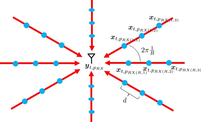
Therefore, for time slot the received signal can be expressed as:
| (1) |
where is the received signal power at position . The terms represent the virtual signal source at position . Additionally, denotes the propagation loss from the virtual signal source at position to the receiver at position . Note that the propagation loss is independent of . It depends only on the distance between the virtual signal source and the receiver.
The notation refers to the position of the th sample on the th ray for the receiver placed at . Specifically, there are virtual signal sources that contribute to the received signal at and their corresponding positions are given by:
| (2) |
where is the sampling resolution on the ray. The propagation loss for the virtual signal source toward receiver position is:
| (3) |
where is the parameter for the transmission medium. In this work, we adopt a simple path loss model as in [18]. A more accurate model could be used if additional information, such as the transmission frequency, is available.
For notation simplicity, we rewrite the received signal model for time slot (1) into vector form:
| (4) |
3.3 Gaussian Random Field
For a given time slot , we model the RF Radiance Field as a Gaussian random process, with the virtual signal sources—components of the RF Radiance Field—modeled as Gaussian random variables. A Gaussian process is characterized by its mean and covariance (also referred to as the kernel):
-
•
Mean: For any position , the virtual signal is modeled as a zero-mean Gaussian random variable.
(5) -
•
Covariance: The covariance between each pair of virtual signal sources is given by:
(6)
The value of represents the variance of the virtual signal sources, which are selected based on the true transmission power of the device within the room. The length-scale parameter , controls the rate of variation of the signal; smaller values of indicate a sharper change in the function. In a later section, we will demonstrate how to estimate this parameter. Note that (6) represents the Radial Basis Function (RBF) kernel. For information on other types of kernel functions and guidance on selecting the appropriate kernel, we refer the reader to [13].
With the above definitions, , the collection of virtual signal sources contributing to is a Gaussian random vector:
| (7) |
Here, is the covariance matrix where the th component represents the covariance between the and components of .
Also, , a linear combination of Gaussian random variables. (4) is a Gaussian random variable with the following distribution:
| (8) |
3.4 Conventional Gaussian Prediction
Next, we describe how to predict the received signal power at a given target position using observations , within the same time slot . Since the observation is a Gaussian random variable, the collection of observations can be represented as a Gaussian random vector:
| (9) |
where represents the collection of virtual signal sources contributing to the observations for time slot :
| (10) |
The matrix is the linear combination matrix, given by:
| (11) |
where is the identity matrix and represents the Kronecker product.
Next, by stacking the the received signal power for the target position into (9), we obtain a new Gaussian random vector:
| (18) |
The mean and covariance matrix can be computed using (8). We denote this distribution as:
With (26), the predicted value for the target position can be calculated using the conditional probability formula:
| (27) |
-
•
Prediction Mean:
(28) -
•
Prediction Variance:
(29)
Notice that in (29), the prediction variance at the selected target position depends only on the target position and the locations of all previously sampled observations.
4 Methods
In this section, we demonstrate how the aforementioned model can be used to reconstruct the RF Radiance Field. Our approach consists of three main parts: Local Kernel Estimation, Active Sampling, and Quasi-Dynamic Reconstruction. In the first part, we use the given observations to reconstruct the RF Radiance Field with a more precise uncertainty model compared to equation (29). Next, leveraging this uncertainty model, we show how observations can be collected more efficiently. Finally, we demonstrate that when the RF Radiance Field changes from time slot to , only a few new samples are needed to reconstruct the updated field.
4.1 Local Kernel Estimation
From the conventional Gaussian prediction, it is shown that if the kernel function is given, we can obtain both the prediction mean and the prediction variance for any given target position. The computational bottleneck arises from the inverse operation of the matrix in (28) and (29). The size of for observations is . As a result, the computational complexity is . This complexity is particularly high in large-scale radiance fields which entail a large number of observations.
Moreover, in a given scene, certain areas may consist of empty space, where virtual signal sources are expected to be highly correlated. In contrast, other areas may be densely populated with objects such as tables, chairs, and other furniture. In these crowded regions, the correlation between virtual signal sources will differ from that in the empty spaces. As a result, the uncertainty model should be adapted based on the characteristics of the observations. Specifically, we assign low uncertainty to smoother areas and higher uncertainty to regions with sharper variations.
To address the two issues mentioned above, we propose a local kernel estimation strategy that tackles both the computational complexity and the correlation locality problems. For a selected target position , we use only the past observations sampled close to to perform the local kernel estimation and predict . Specifically, observation will be used for the local kernel estimation for position , if the position of the observation, , is sufficiently close , that is:
| (30) |
Here, is the locality parameter, which can be set based on the complexity of the scene structure or learned from the RF Radiance Fields of other scenes. In this work, we present the concept of local kernel estimation, leaving the determination of the optimal value for for future work.
Once the observations for the selected target are obtained, we need to estimate the kernel’s length-scale parameter , as shown in (6). However, since we are now performing local kernel estimation, this length-scale parameter should depend on the position of the target. Therefore, we modify (6) as follows:
| (31) |
Next, we perform maximum likelihood estimation to estimate the local length-scale parameter in (31):
| (32) |
where is a subset of that satisfies the condition in (30) and denotes the number of elements of .
Now that we have estimated the local kernel from the local samples near the selected target, we can apply (28) and (29) to obtain the prediction mean and variance of .
Since only observations are used for the prediction, the computation complexity is reduced from to . If the observations are uniformly distributed within the room, then the ratio is approximately, where is the locality parameter.
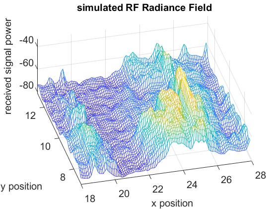
To illustrate the concept of local kernel estimation, we use simulated data from the NeRF2 pre-trained model, which models a room measuring room, , as shown in Fig.4. The room contains 200 randomly distributed observations. We set the locality parameter for the local kernel estimation. As shown in Fig 2, only 7 observations are used to predict the received signal at the selected target.
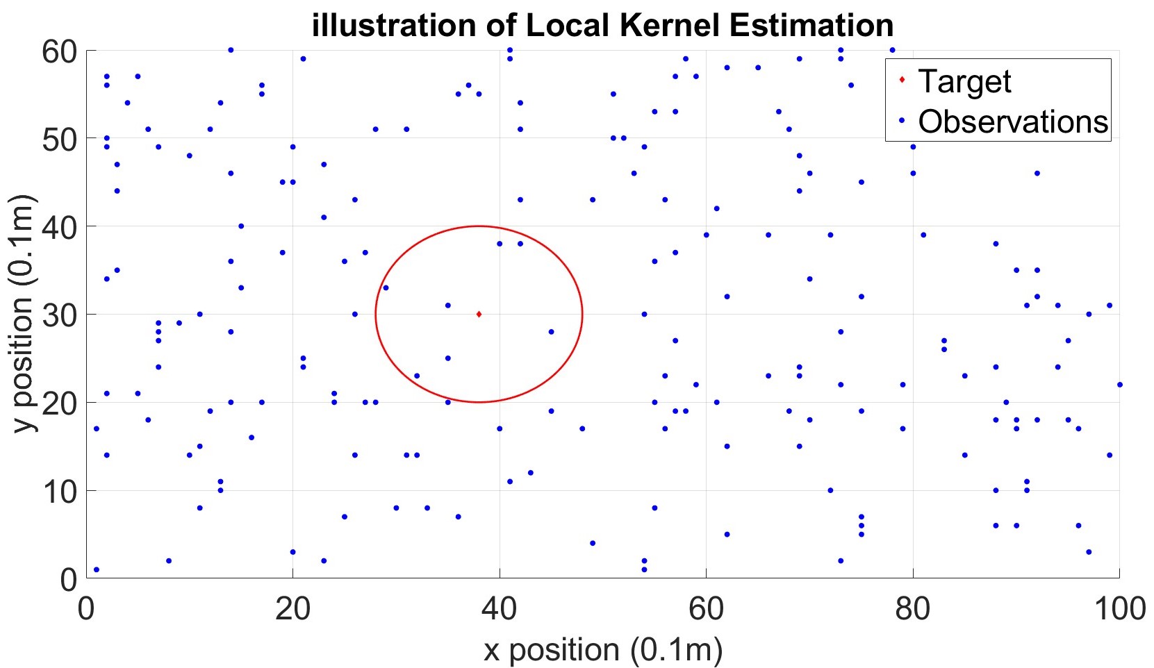
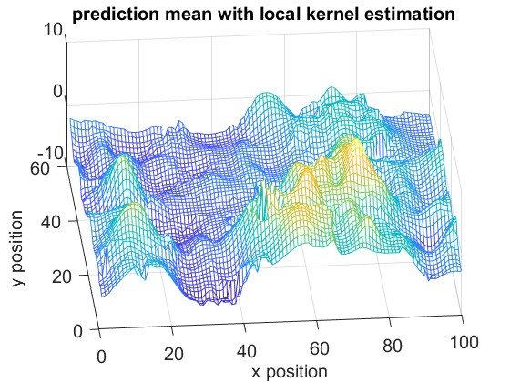
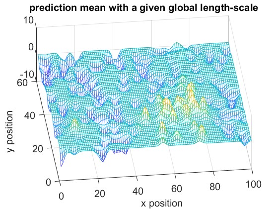
Fig. 6 and Fig. 6 shows the reconstruction of the RF Radiance Field with and without our proposed local kernel estimation. The results demonstrate that our method effectively captures the sharp details of the RF Radiance Field, leading to a more accurate reconstruction.
4.2 Active Sampling
As shown in the previous section, we can predict the mean and variance of the RF Radiance Field at any selected target position based on a given set of observations. However, collecting these observations can be expensive, and some may provide limited or negligible information. In such cases, adding these samples to the reconstruction may have little effect on the model’s accuracy. To address this, we propose an active sampling strategy for collecting more informative observations.
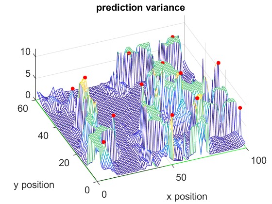
Our approach begins by making an initial prediction of the radiance field using a small number of randomly selected observations. We then adaptively choose the next observation position based on the highest predicted variance, as given by (29). Fig. 4 shows an example of the prediction variance of the received signal power across different positions. After a few initial observations, only certain areas of the scene exhibit high uncertainty (i.e., large variance). Thus, further observations are focused on these high-variance regions to improve the model’s accuracy most efficiently. The proposed method for static RF Radiance Field is summarize in Alg. 1. In this work, instead of only selecting the largest variance position each time, we divide the scene into smaller sections and select the position with the highest variance within each section as the next observation point. This approach helps avoid repeatedly computing the matrix inverse in (28) and (29) by adding only one new observation at a time. Note that some sections may be skipped if the predicted variances of all positions within a section are below a certain threshold. By combining Local Kernel Estimation with Active Sampling, we learn the sharpness of different regions of the RF Radiance Field and focus more observations on the areas with higher sharpness. Since smoother regions can be predicted with fewer samples, active sampling allows us to reduce the overall number of samples.
Input:
-
•
: Initial number of observations
-
•
targets: Set of target positions
Output: Prediction mean and variance for each target position
Initialize: Collect initial observations
For each target position in targets:
4.3 Quasi-Dynamic Reconstruction
Now, we explore the potential of our proposed method in a quasi-dynamic environment. We focus on the scenario where the RF Radiance Field of the scene has already been fully measured for time slot , and at time slot , some parts of the RF Radiance Field have changed due to environmental dynamics. The received signal power at a target position can be written as:
| (33) |
where denotes the difference of the value between time slot and for position .
In the previous static case, our proposed Local Kernel Estimation and Active Sampling methods learned the sharpness of the RF Radiance Field, focusing more on the sharp areas. However, when transitioning from time slot to , the sharp areas of the RF Radiance Field might remain the same. If we continue to focus on these areas of sharpness, we may end up observing unchanged regions. Therefore, instead of learning the structure of the new RF Radiance Field, we apply our method to learn the difference between the RF Radiance Fields at time slots and time slot . As shown in (33), we can obtain by learning the difference . By focusing on the differences between the two time slots, our method prioritizes regions with significant changes, which is exactly what is needed to adapt to the evolving RF Radiance Field.
5 Experiments
In this section, we present the simulation results of our proposed method and compare it with NeRF2.
Experimental Setup and Data Collection. We evaluate four different scenarios, corresponding to rooms of sizes , , , and respectively. Our experiments involve both real and simulated data for the first three scenarios. The real data comes from three different rooms in the NeRF2 dataset, with , , and samples, respectively. The simulated data is generated from the NeRF2 pre-trained model for the same three rooms, with a resolution of . The fourth scenario involves real RSSI data measured in a meeting room. We utilize a Turtlebot4 robot equipped with Lidar and SLAM capabilities as our mobile platform. The robot carries two key wireless systems: a 60 GHz mmWave system using MikroTik wAP 60G×3 routers, and a 5 GHz WiFi system consisting of an 802.11ac access point and an LG Nexus 5 smartphone using CSIKit for RSSI extraction. We measure real RSSI data in a meeting room.
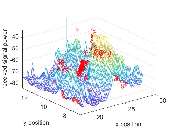
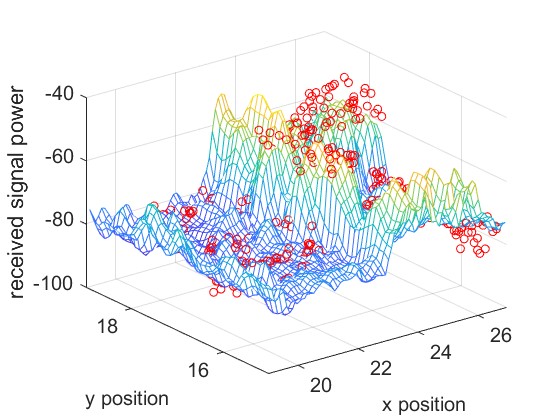
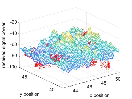
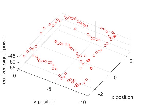
The ground truth of the received signal power for different scenarios is shown in Fig. 7. The mesh plot represents the simulated data for the entire space, while the red dots indicate the real data.
For the quasi-dynamic case, we used the simulated data from Scenario 1 as the RF Radiance Field for time slot and introduced a random bias term to model the RF Radiance Field for time slot .
Evaluation Metrics We computed the Median Absolute Error (Median AE) and the Mean Absolute Error (MAE) across the entire room, excluding the observations (training set), using a resolution for the simulated data. For the real data, we evaluated the errors at all sampled positions, excluding the observations(training set).
5.1 Results
Here, we present the results of the experiment for both static and quasi-dynamic RF Radiance Fields.
5.1.1 Static RF Radiance Field
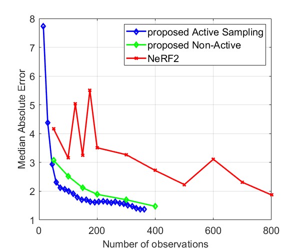
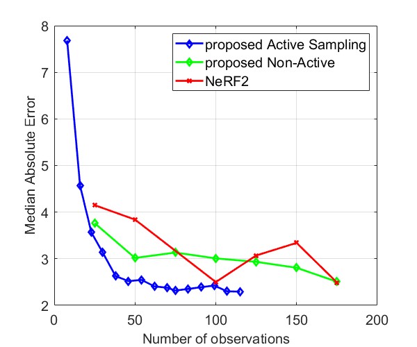
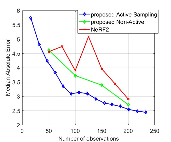
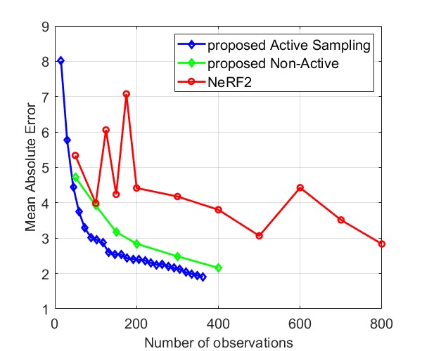
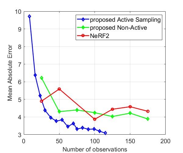
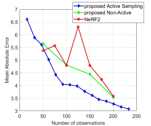
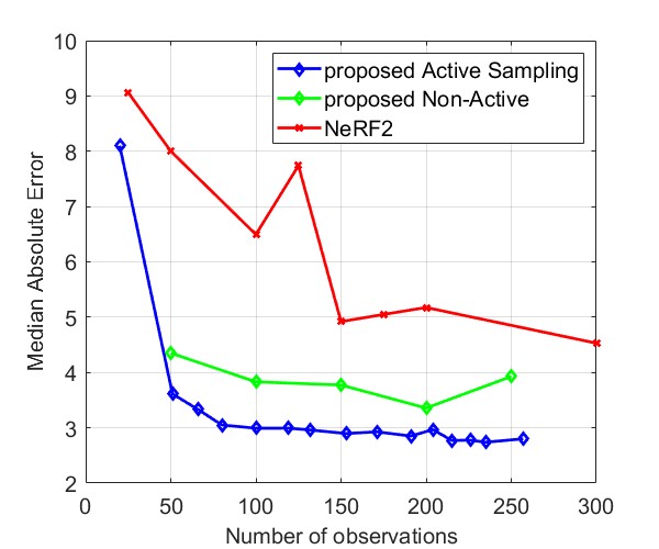
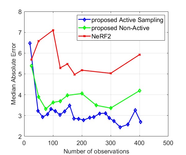
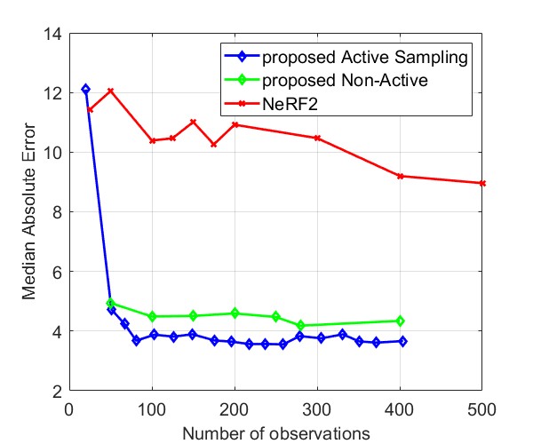
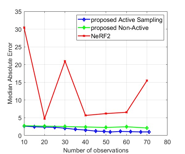
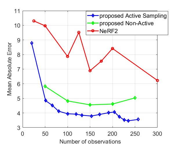
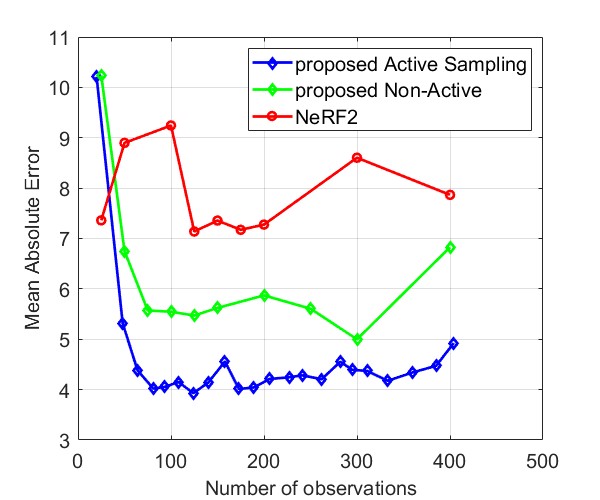
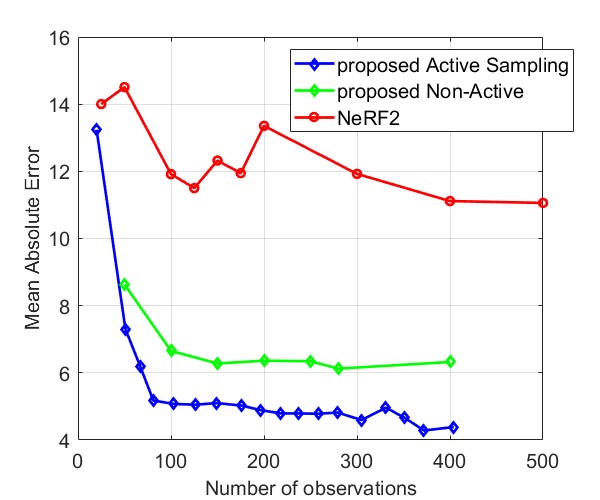
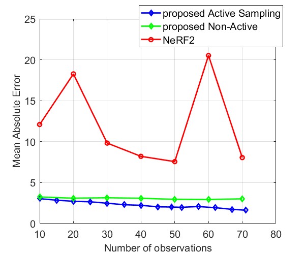
Fig. 8 and Fig. 9 compare the Median AE and MAE between our proposed method and NeRF2, using simulated data and real data, respectively. The results for simulated data show that our method outperforms NeRF2, reducing the number of observations by . Additionally, our method demonstrates much more stable performance, whereas NeRF2’s performance can vary significantly with small changes in the number of samples. Additionally, the results show that active learning further improves performance by prioritizing positions with high uncertainty. For real data, our method shows substantial improvements in both MAE and Median AE. Since it is challenging to collect a large number of samples in real-world settings, such as inside a room, our method is better suited for practical applications.
5.1.2 Quasi-Dynamic RF Radiance Field
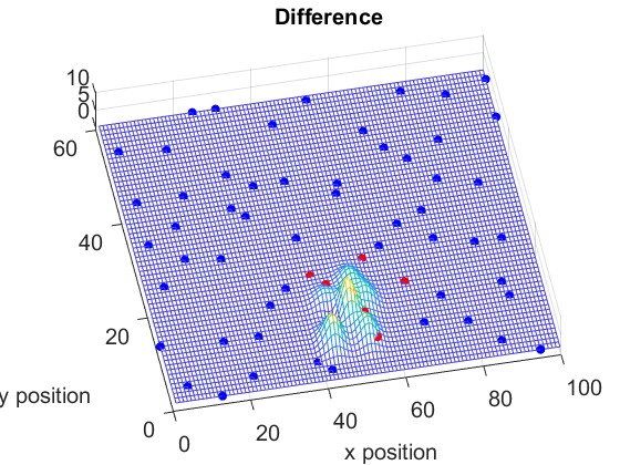
Fig. 11 and Fig. 11 illustrate the RF Radiance Field at time slots and , respectively. Fig. 13 shows the difference of the RF Radiance Field between two time slots.
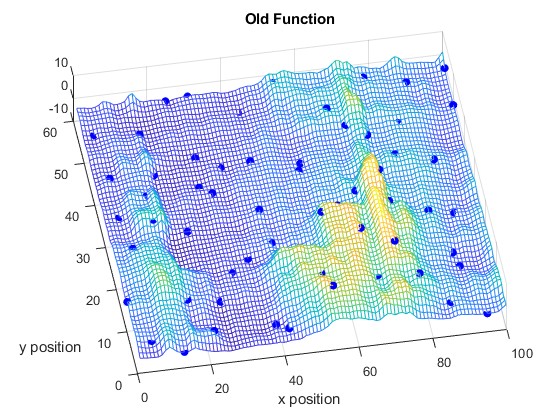
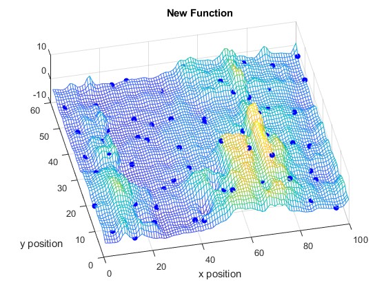
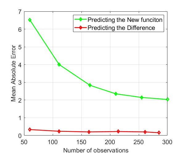
We compare the Mean Absolute Error (MAE) of learning the new RF Radiance Field versus learning the difference in Fig. 13. It shows that our proposed method requires only a few samples to learn the change in the RF Radiance Field, making it highly suitable for practical applications. Additionally, unlike NeRF2, which requires several hours to train a model, our method allows for immediate reconstruction of the RF Radiance Field as soon as new observations are available.
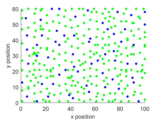
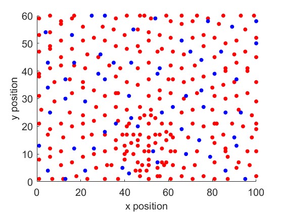
Fig. 15 and Fig. 15 show the positions of the first 300 observations for learning the new function directly and for learning the difference in the function, respectively. As shown in Fig. 15, most of the activated sensors are located near the areas where the RF Radiance Field has changed, which is illustrated in Fig. 13. Note that here, we plot the same number of selected observations to compare their distribution. By learning the difference function, only a few samples are needed to achieve good performance, as shown in Fig. 13.
6 Discussion
Cost of Matrix Inversion. As shown in (28) and (29), our method requires a matrix inversion. When more samples are collected within a small area, this matrix inversion may become problematic, as we currently rely on a brute-force approach. However, it is important to note that this matrix is a covariance matrix with special properties, such as a Toeplitz structure. Iterative methods could be explored to compute the matrix inverse more efficiently.
Furthermore, the proposed local kernel estimation reduces the size of the matrix, making the computation more manageable. Consequently, selecting a smaller locality parameter could be another option. In areas with a high sample density, a smaller can provide higher resolution, capturing finer details and sharpness in the RF Radiance Field.
7 Conclusions
In this work, we propose a training-free method for predicting received signal power in RF Radiance Fields. Our approach quickly generates predictions at any location in the scene and includes an uncertainty model. By using local kernel estimation, it is more computationally efficient than traditional Gaussian prediction methods. Simulation results demonstrate that fewer samples are needed to achieve performance on par with NeRF2. We further reduce the number of observations required by incorporating active sampling, which selects the most informative samples. Finally, our method is well-suited for dynamic scenes. Unlike other neural network-based approaches that require retraining, our method adapts by leveraging new observations to track changes in the scene.
References
- Chan et al. [2019] Shunsuke Chan, Shunsuke Saito, Lingyu Li, Hao Zhao, Shigeo Xiao, Kenji Sugimoto, Shohei Sakashita, and Taku Komura. Pifu: Pixel-aligned implicit function for high-resolution clothed human digitization. Proceedings of the IEEE/CVF International Conference on Computer Vision, 2019.
- Chen et al. [2024] Xingyu Chen, Zihao Feng, Ke Sun, Kun Qian, and Xinyu Zhang. Rfcanvas: Modeling rf channel by fusing visual priors and few-shot rf measurements. In Proceedings of the 22nd ACM Conference on Embedded Networked Sensor Systems, pages 464–477, 2024.
- Egea-Lopez et al. [2021] Esteban Egea-Lopez, Jose Maria Molina-Garcia-Pardo, Martine Lienard, and Pierre Degauque. Opal: An open source ray-tracing propagation simulator for electromagnetic characterization. Plos one, 16(11):e0260060, 2021.
- Hu et al. [2023] Jingzhi Hu, Tianyue Zheng, Zhe Chen, Hongbo Wang, and Jun Luo. Muse-fi: Contactless muti-person sensing exploiting near-field wi-fi channel variation. In Proceedings of the ACM MobiCom, 2023.
- Kerbl et al. [2023] Bernhard Kerbl, Georgios Kopanas, Thomas Leimkühler, and George Drettakis. 3d gaussian splatting for real-time radiance field rendering. ACM Trans. Graph., 42(4):139–1, 2023.
- Mildenhall et al. [2020] Ben Mildenhall, Pratul P Srinivasan, Matthew Tancik, Jonathan T Barron, Ravi Ramamoorthi, and Ren Ng. Nerf: Representing scenes as neural radiance fields for view synthesis. In European Conference on Computer Vision, 2020.
- Mildenhall et al. [2021] Ben Mildenhall, Pratul P Srinivasan, Matthew Tancik, Jonathan T Barron, Ravi Ramamoorthi, and Ren Ng. Nerf: Representing scenes as neural radiance fields for view synthesis. Communications of the ACM, 65(1):99–106, 2021.
- Orekondy et al. [2023] Tribhuvanesh Orekondy, Pratik Kumar, Shreya Kadambi, Hao Ye, Joseph Soriaga, and Arash Behboodi. Winert: Towards neural ray tracing for wireless channel modelling and differentiable simulations. In The Eleventh International Conference on Learning Representations, 2023.
- Park et al. [2019] Jeong Joon Park, Peter Florence, Julian Straub, Richard Newcombe, and Steven Lovegrove. Deepsdf: Learning continuous signed distance functions for shape representation. Proceedings of the IEEE/CVF Conference on Computer Vision and Pattern Recognition, 2019.
- Sitzmann et al. [2020] Vincent Sitzmann, Julien N.P. Martel, Alexander W. Bergman, David B. Lindell, and Gordon Wetzstein. Implicit neural representations with periodic activation functions. In Advances in Neural Information Processing Systems, 2020.
- Tewari et al. [2020] Ayush Tewari, Ohad Fried, Justus Thies, Vincent Sitzmann, Stephen Lombardi, Kalyan Sunkavalli, Ricardo Martin-Brualla, Tomas Simon, Jason Saragih, Matthias Nießner, et al. State of the art on neural rendering. Computer Graphics Forum, 39(2), 2020.
- Vakalis et al. [2019] Stavros Vakalis, Liang Gong, and Jeffrey A Nanzer. Imaging with wifi. IEEE Access, 7:28616–28624, 2019.
- Williams and Rasmussen [2006] Christopher KI Williams and Carl Edward Rasmussen. Gaussian processes for machine learning. MIT press Cambridge, MA, 2006.
- Woodford et al. [2022] Timothy Woodford, Xinyu Zhang, Eugene Chai, and Karthikeyan Sundaresan. Mosaic: Leveraging diverse reflector geometries for omnidirectional around-corner automotive radar. In Proceedings of the 20th Annual International Conference on Mobile Systems, Applications and Services (MobiSys), 2022.
- Xie et al. [2021] Yiheng Xie, Towaki Takikawa, Shunsuke Saito, Or Litany, Shiqin Yan, Numair Khan, Federico Tombari, James Tompkin, Vincent Sitzmann, and Srinath Sridhar. Neural fields in visual computing and beyond. In Computer Graphics Forum, 2021.
- Yariv et al. [2020] Lior Yariv, Yoni Kasten, Dror Moran, Meirav Galun, Matan Atzmon, Basri Ronen, and Yaron Lipman. Multiview neural surface reconstruction by disentangling geometry and appearance. In Advances in Neural Information Processing Systems, 2020.
- Zhao et al. [2022] Hanying Zhao, Mingtao Huang, and Yuan Shen. High-accuracy localization in multipath environments via spatio-temporal feature tensorization. IEEE Transactions on Wireless Communications, 21(12):10576–10591, 2022.
- Zhao et al. [2023] Xiaopeng Zhao, Zhenlin An, Qingrui Pan, and Lei Yang. Nerf2: Neural radio-frequency radiance fields. In Proceedings of the 29th Annual International Conference on Mobile Computing and Networking, pages 1–15, 2023.