Ad Hoc Table Retrieval using Semantic Similarity
Abstract.
We introduce and address the problem of ad hoc table retrieval: answering a keyword query with a ranked list of tables. This task is not only interesting on its own account, but is also being used as a core component in many other table-based information access scenarios, such as table completion or table mining. The main novel contribution of this work is a method for performing semantic matching between queries and tables. Specifically, we (i) represent queries and tables in multiple semantic spaces (both discrete sparse and continuous dense vector representations) and (ii) introduce various similarity measures for matching those semantic representations. We consider all possible combinations of semantic representations and similarity measures and use these as features in a supervised learning model. Using a purpose-built test collection based on Wikipedia tables, we demonstrate significant and substantial improvements over a state-of-the-art baseline.
1. Introduction
Tables are a powerful, versatile, and easy-to-use tool for organizing and working with data. Because of this, a massive number of tables can be found “out there,” on the Web or in Wikipedia, representing a vast and rich source of structured information. Recently, a growing body of work has begun to tap into utilizing the knowledge contained in tables. A wide and diverse range of tasks have been undertaken, including but not limited to (i) searching for tables (in response to a keyword query (Cafarella et al., 2008b; Cafarella et al., 2009; Venetis et al., 2011; Pimplikar and Sarawagi, 2012; Balakrishnan et al., 2015; Nguyen et al., 2015) or a seed table (Das Sarma et al., 2012)), (ii) extracting knowledge from tables (such as RDF triples (Munoz et al., 2014)), and (iii) augmenting tables (with new columns (Das Sarma et al., 2012; Cafarella et al., 2009; Lehmberg et al., 2015; Yakout et al., 2012; Bhagavatula et al., 2013; Zhang and Balog, 2017b), rows (Das Sarma et al., 2012; Yakout et al., 2012; Zhang and Balog, 2017b), cell values (Ahmadov et al., 2015), or links to entities (Bhagavatula et al., 2015)).
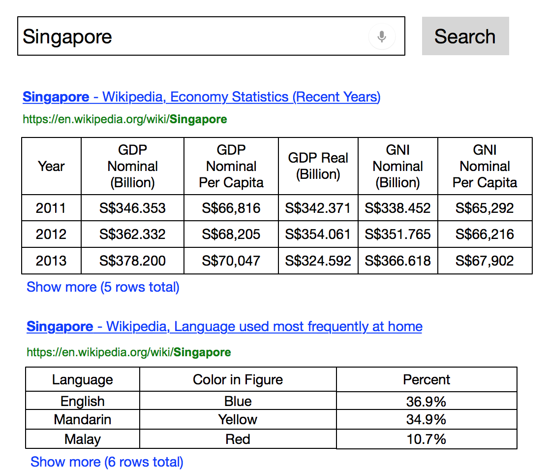
Searching for tables is an important problem on its own, in addition to being a core building block in many other table-related tasks. Yet, it has not received due attention, and especially not from an information retrieval perspective. This paper aims to fill that gap. We define the ad hoc table retrieval task as follows: given a keyword query, return a ranked list of tables from a table corpus that are relevant to the query. See Fig. 1 for an illustration.
It should be acknowledged that this task is not entirely new, in fact, it has been around for a while in the database community (also known there as relation ranking) (Cafarella et al., 2008b; Cafarella et al., 2009; Venetis et al., 2011; Bhagavatula et al., 2013). However, public test collections and proper evaluation methodology are lacking, in addition to the need for better ranking techniques.
Tables can be ranked much like documents, by considering the words contained in them (Cafarella et al., 2008b; Cafarella et al., 2009; Pimplikar and Sarawagi, 2012). Ranking may be further improved by incorporating additional signals related to table quality. Intuitively, high quality tables are topically coherent; other indicators may be related to the pages that contain them (e.g., if they are linked by other pages (Bhagavatula et al., 2013)). However, a major limitation of prior approaches is that they only consider lexical matching between the contents of tables and queries. This gives rise to our main research objective: Can we move beyond lexical matching and improve table retrieval performance by incorporating semantic matching?
We consider two main kinds of semantic representations. One is based on concepts, such as entities and categories. Another is based on continuous vector representations of words and of entities (i.e., word and graph embeddings). We introduce a framework that handles matching in different semantic spaces in a uniform way, by modeling both the table and the query as sets of semantic vectors. We propose two general strategies (early and late fusion), yielding four different measures for computing the similarity between queries and tables based on their semantic representations.
As we have mentioned above, another key area where prior work has insufficiencies is evaluation. First, there is no publicly available test collection for this task. Second, evaluation has been performed using set-based metrics (counting the number of relevant tables in the top- results), which is a very rudimentary way of measuring retrieval effectiveness. We address this by developing a purpose-built test collection, comprising of 1.6M tables from Wikipedia, and a set of queries with graded relevance judgments. We establish a learning-to-rank baseline that encompasses a rich set of features from prior work, and outperforms the best approaches known in the literature. We show that the semantic matching methods we propose can substantially and significantly improve retrieval performance over this strong baseline.
In summary, this paper makes the following contributions:
-
•
We introduce and formalize the ad hoc table ranking task, and present both unsupervised and supervised baseline approaches (Sect. 2).
-
•
We present a set of novel semantic matching methods that go beyond lexical similarity (Sect. 3).
- •
The test collection and the outputs of the reported methods are made available at https://github.com/iai-group/www2018-table.
2. Ad Hoc Table Retrieval
We formalize the ad hoc table retrieval task, explain what information is associated with a table, and introduce baseline methods.
2.1. Problem Statement
Given a keyword query , ad hoc table retrieval is the task of returning a ranked list of tables, , from a collection of tables . Being an ad hoc task, the relevance of each returned table is assessed independently of all other returned tables . Hence, the ranking of tables boils down to the problem of assigning a score to each table in the corpus: . Tables are then sorted in descending order of their scores.
2.2. The Anatomy of a Table
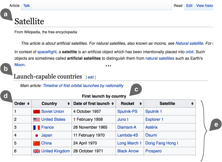
We shall assume that the following information is available for each table in the corpus; the letters refer to Figure 2.
-
(a)
Page title, where the table was extracted from.
-
(b)
Section title, i.e., the heading of the particular section where the table is embedded.
-
(c)
Table caption, providing a brief explanation.
-
(d)
Table headings, i.e., a list of column heading labels.
-
(e)
Table body, i.e., all table cells (including column headings).
2.3. Unsupervised Ranking
An easy and straightforward way to perform the table ranking task is by adopting standard document ranking methods. Cafarella et al. (2009); Cafarella et al. (2008b) utilize web search engines to retrieve relevant documents; tables are then extracted from the highest-ranked documents. Rather than relying on external services, we represent tables as either single- or multi-field documents and apply standard documents retrieval techniques.
| Query features | Source | Value | |
| QLEN | Number of query terms | (Tyree et al., 2011) | {1,…,n} |
| Sum of query IDF scores in field | (Qin et al., 2010) | ||
| Table features | |||
| #rows | The number of rows in the table | (Cafarella et al., 2008b; Bhagavatula et al., 2013) | {1,…,n} |
| #cols | The number of columns in the table | (Cafarella et al., 2008b; Bhagavatula et al., 2013) | {1,…,n} |
| #of NULLs in table | The number of empty table cells | (Cafarella et al., 2008b; Bhagavatula et al., 2013) | {0,…,n} |
| PMI | The ACSDb-based schema coherency score | (Cafarella et al., 2008b) | |
| inLinks | Number of in-links to the page embedding the table | (Bhagavatula et al., 2013) | {0,…,n} |
| outLinks | Number of out-links from the page embedding the table | (Bhagavatula et al., 2013) | {0,…,n} |
| pageViews | Number of page views | (Bhagavatula et al., 2013) | {0,…,n} |
| tableImportance | Inverse of number of tables on the page | (Bhagavatula et al., 2013) | |
| tablePageFraction | Ratio of table size to page size | (Bhagavatula et al., 2013) | |
| Query-table features | |||
| #hitsLC | Total query term frequency in the leftmost column cells | (Cafarella et al., 2008b) | {0,…,n} |
| #hitsSLC | Total query term frequency in second-to-leftmost column cells | (Cafarella et al., 2008b) | {0,…,n} |
| #hitsB | Total query term frequency in the table body | (Cafarella et al., 2008b) | {0,…,n} |
| qInPgTitle | Ratio of the number of query tokens found in page title to total number of tokens | (Bhagavatula et al., 2013) | |
| qInTableTitle | Ratio of the number of query tokens found in table title to total number of tokens | (Bhagavatula et al., 2013) | |
| yRank | Rank of the table’s Wikipedia page in Web search engine results for the query | (Bhagavatula et al., 2013) | {1,…,n} |
| MLM similarity | Language modeling score between query and multi-field document repr. of the table | (Chen et al., 2016) | (,0) |
2.3.1. Single-field Document Representation
In the simplest case, all text associated with a given table is used as the table’s representation. This representation is then scored using existing retrieval methods, such as BM25 or language models.
2.3.2. Multi-field Document Representation
Rather than collapsing all textual content into a single-field document, it may be organized into multiple fields, such as table caption, table headers, table body, etc. (cf. Sect. 2.2). For multi-field ranking, Pimplikar and Sarawagi (2012) employ a late fusion strategy (Zhang and Balog, 2017a). That is, each field is scored independently against the query, then a weighted sum of the field-level similarity scores is taken:
| (1) |
where denotes the th (document) field for table and is the corresponding field weight (such that ). may be computed using any standard retrieval method. We use language models in our experiments.
2.4. Supervised Ranking
The state-of-the-art in document retrieval (and in many other retrieval tasks) is to employ supervised learning (Liu, 2011). Features may be categorized into three groups: (i) document, (ii) query, and (iii) query-document features (Qin et al., 2010). Analogously, we distinguish between three types of features: (i) table, (ii) query, and (iii) query-table features. In Table 1, we summarize the features from previous work on table search (Cafarella et al., 2008b; Bhagavatula et al., 2013). We also include a number of additional features that have been used in other retrieval tasks, such as document and entity ranking; we do not regard these as novel contributions.
2.4.1. Query Features
Query features have been shown to improve retrieval performance for document ranking (Macdonald et al., 2012). We adopt two query features from document retrieval, namely, the number of terms in the query (Tyree et al., 2011), and query IDF (Qin et al., 2010) according to: , where is the IDF score of term in field . This feature is computed for the following fields: page title, section title, table caption, table heading, table body, and “catch-all” (the concatenation of all textual content in the table).
2.4.2. Table Features
Table features depend only on the table itself and aim to reflect the quality of the given table (irrespective of the query). Some features are simple characteristics, like the number of rows, columns, and empty cells (Cafarella et al., 2008b; Bhagavatula et al., 2013). A table’s PMI is computed by calculating the PMI values between all pairs of column headings of that table, and then taking their average. Following (Cafarella et al., 2008b), we compute PMI by obtaining frequency statistics from the Attribute Correlation Statistics Database (ACSDb) (Cafarella et al., 2008a), which contains table heading information derived from millions of tables extracted from a large web crawl.
Another group of features has to do with the page that embeds the table, by considering its connectivity (inLinks and outLinks), popularity (pageViews), and the table’s importance within the page (tableImportance and tablePageFraction).
2.4.3. Query-Table Features
Features in the last group express the degree of matching between the query and a given table. This matching may be based on occurrences of query terms in the page title (qInPgTitle) or in the table caption (qInTableTitle). Alternatively, it may be based on specific parts of the table, such as the leftmost column (#hitsLC), second-to-left column (#hitsSLC), or table body (#hitsB). Tables are typically embedded in (web) pages. The rank at which a table’s parent page is retrieved by an external search engine is also used as a feature (yRank). (In our experiments, we use the Wikipedia search API to obtain this ranking.) Furthermore, we take the Mixture of Language Models (MLM) similarity score (Ogilvie and Callan, 2003) as a feature, which is actually the best performing method among the four text-based baseline methods (cf. Sect. 5). Importantly, all these features are based on lexical matching. Our goal in this paper is to also enable semantic matching; this is what we shall discuss in the next section.
3. Semantic Matching
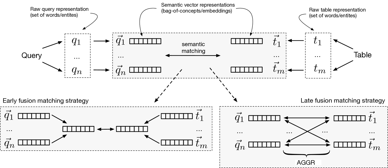
This section presents our main contribution, which is a set of novel semantic matching methods for table retrieval. The main idea is to go beyond lexical matching by representing both queries and tables in some semantic space, and measuring the similarity of those semantic (vector) representations. Our approach consists of three main steps, which are illustrated in Figure 3. These are as follows (moving from outwards to inwards on the figure):
-
(1)
The “raw” content of a query/table is represented as a set of terms, where terms can be either words or entities (Sect. 3.1).
-
(2)
Each of the raw terms is mapped to a semantic vector representation (Sect. 3.2).
-
(3)
The semantic similarity (matching score) between a query-table pair is computed based on their semantic vector representations (Sect. 3.3).
We compute query-table similarity using all possible combinations of semantic representations and similarity measures, and use the resulting semantic similarity scores as features in a learning-to-rank approach. Table 2 summarizes these features.
3.1. Content Extraction
We represent the “raw” content of the query/table as a set of terms, where terms can be either words (string tokens) or entities (from a knowledge base). We denote these as and for query and table , respectively.
3.1.1. Word-based
It is a natural choice to simply use word tokens to represent query/table content. That is, is comprised of the unique words in the query. As for the table, we let contain all unique words from the title, caption, and headings of the table. Mind that at this stage we are only considering the presence/absence of words. During the query-table similarity matching, the importance of the words will also be taken into account (Sect. 3.3.1).
3.1.2. Entity-based
Many tables are focused on specific entities (Zhang and Balog, 2017b). Therefore, considering the entities contained in a table amounts to a meaningful representation of its content. We use the DBpedia knowledge base as our entity repository. Since we work with tables extracted from Wikipedia, the entity annotations are readily available (otherwise, entity annotations could be obtained automatically, see, e.g., (Venetis et al., 2011)). Importantly, instead of blindly including all entities mentioned in the table, we wish to focus on salient entities. It has been observed in prior work (Venetis et al., 2011; Bhagavatula et al., 2015) that tables often have a core column, containing mostly entities, while the rest of the columns contain properties of these entities (many of which are entities themselves). We write to denote the set of entities that are contained in the core column of the table, and describe our core column detection method in Sect. 3.1.3. In addition to the entities taken directly from the body part of the table, we also include entities that are related to the page title () and to the table caption (). We obtain those by using the page title and the table caption, respectively, to retrieve relevant entities from the knowledge base. We write to denote the set of top- entities retrieved for the query . We detail the entity ranking method in Sect. 3.1.4. Finally, the table is represented as the union of three sets of entities, originating from the core column, page title, and table caption: .
To get an entity-based representation for the query, we issue the query against a knowledge base to retrieve relevant entities, using the same retrieval method as above. I.e., .
3.1.3. Core Column Detection
We introduce a simple and effective core column detection method. It is based on the notion of column entity rate, which is defined as the ratio of cells in a column that contain an entity. We write to denote the column entity rate of column in table . Then, the index of the core column becomes: , where is the number of columns in .
3.1.4. Entity Retrieval
We employ a fielded entity representation with five fields (names, categories, attributes, similar entity names, and related entity names) and rank entities using the Mixture of Language Models approach (Ogilvie and Callan, 2003). The field weights are set uniformly. This corresponds to the MLM-all model in (Hasibi et al., 2017b) and is shown to be a solid baseline. We return the top- entities, where is set to 10.
| Features | Semantic repr. | Raw repr. |
|---|---|---|
| Entity_* | Bag-of-entities | entities |
| Category_* | Bag-of-categories | entities |
| Word_* | Word embeddings | words |
| Graph_* | Graph embeddings | entities |
3.2. Semantic Representations
Next, we embed the query/table terms in a semantic space. That is, we map each table term to a vector representation , where refers to the th element of that vector. For queries, the process goes analogously. We discuss two main kinds of semantic spaces, bag-of-concepts and embeddings, with two alternatives within each. The former uses sparse and discrete, while the latter employs dense and continuous-valued vectors. A particularly nice property of our semantic matching framework is that it allows us to deal with these two different types of representations in a unified way.
3.2.1. Bag-of-concepts
One alternative for moving from the lexical to the semantic space is to represent tables/queries using specific concepts. In this work, we use entities and categories from a knowledge base. These two semantic spaces have been used in the past for various retrieval tasks, in duet with the traditional bag-of-words content representation. For example, entity-based representations have been used for document retrieval (Xiong et al., 2017; Raviv et al., 2016) and category-based representations have been used for entity retrieval (Balog et al., 2011). One important difference from previous work is that instead of representing the entire query/table using a single semantic vector, we map each individual query/table term to a separate semantic vector, thereby obtaining a richer representation.
We use the entity-based raw representation from the previous section, that is, and are specific entities. Below, we explain how table terms are projected to , which is a sparse discrete vector in the entity/category space; for query terms it follows analogously.
- Bag-of-entities:
-
Each element in corresponds to a unique entity. Thus, the dimensionality of is the number of entities in the knowledge base (on the order of millions). has a value of if entities and are related (there exists a link between them in the knowledge base), and otherwise.
- Bag-of-categories:
-
Each element in corresponds to a Wikipedia category. Thus, the dimensionality of amounts to the number of Wikipedia categories (on the order hundreds of thousands). The value of is if entity is assigned to Wikipedia category , and otherwise.
3.2.2. Embeddings
Recently, unsupervised representation learning methods have been proposed for obtaining embeddings that predict a distributional context, i.e., word embeddings (Mikolov et al., 2013; Pennington et al., 2014) or graph embeddings (Perozzi et al., 2014; Tang et al., 2015; Ristoski and Paulheim, 2016). Such vector representations have been utilized successfully in a range of IR tasks, including ad hoc retrieval (Ganguly et al., 2015; Mitra et al., 2016), contextual suggestion (Manotumruksa et al., 2016), cross-lingual IR (Vulić and Moens, 2015), community question answering (Zhou et al., 2015), short text similarity (Kenter and de Rijke, 2015), and sponsored search (Grbovic et al., 2015). We consider both word-based and entity-based raw representations from the previous section and use the corresponding (pre-trained) embeddings as follows.
- Word embeddings:
-
We map each query/table word to a word embedding. Specifically, we use word2vec (Mikolov et al., 2013) with 300 dimensions, trained on Google News data.
- Graph embeddings:
-
We map each query/table entity to a graph embedding. In particular, we use RDF2vec (Ristoski and Paulheim, 2016) with 200 dimensions, trained on DBpedia 2015-10.
3.3. Similarity Measures
The final step is concerned with the computation of the similarity between a query-table pair, based on the semantic vector representations we have obtained for them. We introduce two main strategies, which yield four specific similarity measures. These are summarized in Table 3.
3.3.1. Early Fusion
The first idea is to represent the query and the table each with a single vector. Their similarity can then simply be expressed as the similarity of the corresponding vectors. We let be the centroid of the query term vectors (). Similarly, denotes the centroid of the table term vectors. The query-table similarity is then computed by taking the cosine similarity of the centroid vectors. When query/table content is represented in terms of words, we additionally make use of word importance by employing standard TF-IDF term weighting. Note that this only applies to word embeddings (as the other three semantic representations are based on entities). In case of word embeddings, the centroid vectors are calculated as . The computation of follows analogously.
| Measure | Equation |
|---|---|
| Early | |
| Late-max | |
| Late-sum | |
| Late-avg |
3.3.2. Late Fusion
Instead of combining all semantic vectors and into a single one, late fusion computes the pairwise similarity between all query and table vectors first, and then aggregates those. We let be a set that holds all pairwise cosine similarity scores: . The query-table similarity score is then computed as , where is an aggregation function. Specifically, we use , and as aggregators; see the last three rows in Table 3 for the equations.
4. Test Collection
We introduce our test collection, including the table corpus, test and development query sets, and the procedure used for obtaining relevance assessments.
4.1. Table Corpus
We use the WikiTables corpus (Bhagavatula et al., 2015), which comprises 1.6M tables extracted from Wikipedia (dump date: 2015 October). The following information is provided for each table: table caption, column headings, table body, (Wikipedia) page title, section title, and table statistics like number of headings rows, columns, and data rows. We further replace all links in the table body with entity identifiers from the DBpedia knowledge base (version 2015-10) as follows. For each cell that contains a hyperlink, we check if it points to an entity that is present in DBpedia. If yes, we use the DBpedia identifier of the linked entity as the cell’s content; otherwise, we replace the link with the anchor text, i.e., treat it as a string.
4.2. Queries
We sample a total of 60 test queries from two independent sources (30 from each): (1) Query subset 1 (QS-1): Cafarella et al. (2009) collected 51 queries from Web users via crowdsourcing (using Amazon’s Mechanical Turk platform, users were asked to suggest topics or supply URLs for a useful data table). (2) Query subset 2 (QS-2): Venetis et al. (2011) analyzed the query logs from Google Squared (a service in which users search for structured data) and constructed 100 queries, all of which are a combination of an instance class (e.g., “laptops”) and a property (e.g., “cpu”). Following (Bhagavatula et al., 2013), we concatenate the class and property fields into a single query string (e.g., “laptops cpu”). Table 4 lists some examples.
4.3. Relevance Assessments
We collect graded relevance assessments by employing three independent (trained) judges. For each query, we pool the top 20 results from five baseline methods (cf. Sect. 5.3), using default parameter settings. (Then, we train the parameters of those methods with help of the obtained relevance labels.) Each query-table pair is judged on a three point scale: 0 (non-relevant), 1 (somewhat relevant), and 2 (highly relevant). Annotators were situated in a scenario where they need to create a table on the topic of the query, and wish to find relevant tables that can aid them in completing that task. Specifically, they were given the following labeling guidelines: (i) a table is non-relevant if it is unclear what it is about (e.g., misses headings or caption) or is about a different topic; (ii) a table is relevant if some cells or values could be used from this table; and (iii) a table is highly relevant if large blocks or several values could be used from it when creating a new table on the query topic.
We take the majority vote as the relevance label; if no majority agreement is achieved, we take the average of the scores as the final label. To measure inter-annotator agreement, we compute the Kappa test statistics on test annotations, which is 0.47. According to (Fleiss et al., 1971), this is considered as moderate agreement. In total, 3120 query-table pairs are annotated as test data. Out of these, 377 are labeled as highly relevant, 474 as relevant, and 2269 as non-relevant.
5. Evaluation
| Method | NDCG@5 | NDCG@10 | NDCG@15 | NDCG@20 |
|---|---|---|---|---|
| Single-field document ranking | 0.4315 | 0.4344 | 0.4586 | 0.5254 |
| Multi-field document ranking | 0.4770 | 0.4860 | 0.5170 | 0.5473 |
| WebTable (Cafarella et al., 2008b) | 0.2831 | 0.2992 | 0.3311 | 0.3726 |
| WikiTable (Bhagavatula et al., 2013) | 0.4903 | 0.4766 | 0.5062 | 0.5206 |
| LTR baseline (this paper) | 0.5527 | 0.5456 | 0.5738 | 0.6031 |
| STR (this paper) | 0.5951 | 0.6293† | 0.6590‡ | 0.6825† |
In this section, we list our research questions (Sect. 5.1), discuss our experimental setup (Sect. 5.2), introduce the baselines we compare against (Sect. 5.3), and present our results (Sect. 5.4) followed by further analysis (Sect. 5.5).
5.1. Research Questions
The research questions we seek to answer are as follows.
- RQ1:
-
Can semantic matching improve retrieval performance?
- RQ2:
-
Which of the semantic representations is the most effective?
- RQ3:
-
Which of the similarity measures performs better?
5.2. Experimental Setup
We evaluate table retrieval performance in terms of Normalized Discounted Cumulative Gain (NDCG) at cut-off points 5, 10, 15, and 20. To test significance, we use a two-tailed paired t-test and write / to denote significance at the 0.05 and 0.005 levels, respectively.
Our implementations are based on Nordlys (Hasibi et al., 2017a). Many of our features involve external sources, which we explain below. To compute the entity-related features (i.e., features in Table 1 as well as the features based on the bag-of-entities and bag-of-categories representations in Table 2), we use entities from the DBpedia knowledge base that have an abstract (4.6M in total). The table’s Wikipedia rank (yRank) is obtained using Wikipedia’s MediaWiki API. The PMI feature is estimated based on the ACSDb corpus (Cafarella et al., 2008a). For the distributed representations, we take pre-trained embedding vectors, as explained in Sect. 3.2.2.
| Sem. Repr. | Early | Late-max | Late-sum | Late-avg | ALL |
|---|---|---|---|---|---|
| Bag-of-entities | 0.6754 (+11.99%) | 0.6407 (+6.23%)† | 0.6697 (+11.04%)‡ | 0.6733 (+11.64%)‡ | 0.6696 (+11.03%)‡ |
| Bag-of-categories | 0.6287 (+4.19%) | 0.6245 (+3.55%) | 0.6315 (+4.71%)† | 0.6240 (+3.47%) | 0.6149 (+1.96%) |
| Word embeddings | 0.6181 (+2.49%) | 0.6328 (+4.92%) | 0.6371 (+5.64%)† | 0.6485 (+7.53%)† | 0.6588 (+9.24%)† |
| Graph embeddings | 0.6326 (+4.89%) | 0.6142 (+1.84%) | 0.6223 (+3.18%) | 0.6316 (+4.73%) | 0.6340 (+5.12%) |
| ALL | 0.6736 (+11.69%)† | 0.6631 (+9.95%)† | 0.6831 (+13.26%)‡ | 0.6809 (+12.90%)‡ | 0.6825 (13.17%)‡ |
5.3. Baselines
We implement four baseline methods from the literature.
- Single-field document ranking:
- Multi-field document ranking:
-
Pimplikar and Sarawagi (2012) represent each table as a fielded document, using five fields: Wikipedia page title, table section title, table caption, table body, and table headings. We use the Mixture of Language Models approach (Ogilvie and Callan, 2003) for ranking. Field weights are optimized using the coordinate ascent algorithm; smoothing parameters are trained for each field individually.
- WebTable:
- WikiTable:
Additionally, we introduce a learning-to-rank baseline:
- LTR baseline:
-
It uses the full set of features listed in Table 1. We employ pointwise regression using the Random Forest algorithm.111We also experimented with Gradient Boosting regression and Support Vector Regression, and observed the same general patterns regarding feature importance. However, their overall performance was lower than that of Random Forests. We set the number of trees to 1000 and the maximum number of features in each tree to 3. We train the model using 5-fold cross-validation (w.r.t. NDCG@20); reported results are averaged over 5 runs.
The baseline results are presented in the top block of Table 5. It can be seen from this table that our LTR baseline (row five) outperforms all existing methods from the literature; the differences are substantial and statistically significant. Therefore, in the remainder of this paper, we shall compare against this strong baseline, using the same learning algorithm (Random Forests) and parameter settings. We note that our emphasis is on the semantic matching features and not on the supervised learning algorithm.
5.4. Experimental Results
The last line of Table 5 shows the results for our semantic table retrieval (STR) method. It combines the baseline set of features (Table 1) with the set of novel semantic matching features (from Table 2, 16 in total). We find that these semantic features bring in substantial and statistically significant improvements over the LTR baseline. Thus, we answer RQ1 positively. The relative improvements range from 7.6% to 15.3%, depending on the rank cut-off.
To answer RQ2 and RQ3, we report on all combinations of semantic representations and similarity measures in Table 6. In the interest of space, we only report on NDCG@20; the same trends were observed for other NDCG cut-offs. Cells with a white background show retrieval performance when extending the LTR baseline with a single feature. Cells with a grey background correspond to using a given semantic representation with different similarity measures (rows) or using a given similarity measure with different semantic representations (columns). The first observation is that all features improve over the baseline, albeit not all of these improvements are statistically significant. Concerning the comparison of different semantic representations (RQ2), we find that bag-of-entities and word embeddings achieve significant improvements; see the rightmost column of Table 6. It is worth pointing out that for word embeddings the four similarity measures seem to complement each other, as their combined performance is better than that of any individual method. It is not the case for bag-of-entities, where only one of the similarity measures (Late-max) is improved by the combination. Overall, in answer to RQ2, we find the bag-of-entities representation to be the most effective one. The fact that this sparse representation outperforms word embeddings is regarded as a somewhat surprising finding, given that the latter has been trained on massive amounts of (external) data.
As for the choice of similarity measure (RQ3), it is difficult to name a clear winner when a single semantic representation is used. The relative differences between similarity measures are generally small (below 5%). When all four semantic representations are used (bottom row in Table 6), we find that Late-sum and Late-avg achieve the highest overall improvement. Importantly, when using all semantic representations, all four similarity measures improve significantly and substantially over the baseline. We further note that the combination of all similarity measures do not yield further improvements over Late-sum or Late-avg. In answer to RQ3, we identify the late fusion strategy with sum or avg aggregation (i.e., Late-sum or Late-avg) as the preferred similarity method.
5.5. Analysis
We continue with further analysis of our results.
5.5.1. Features
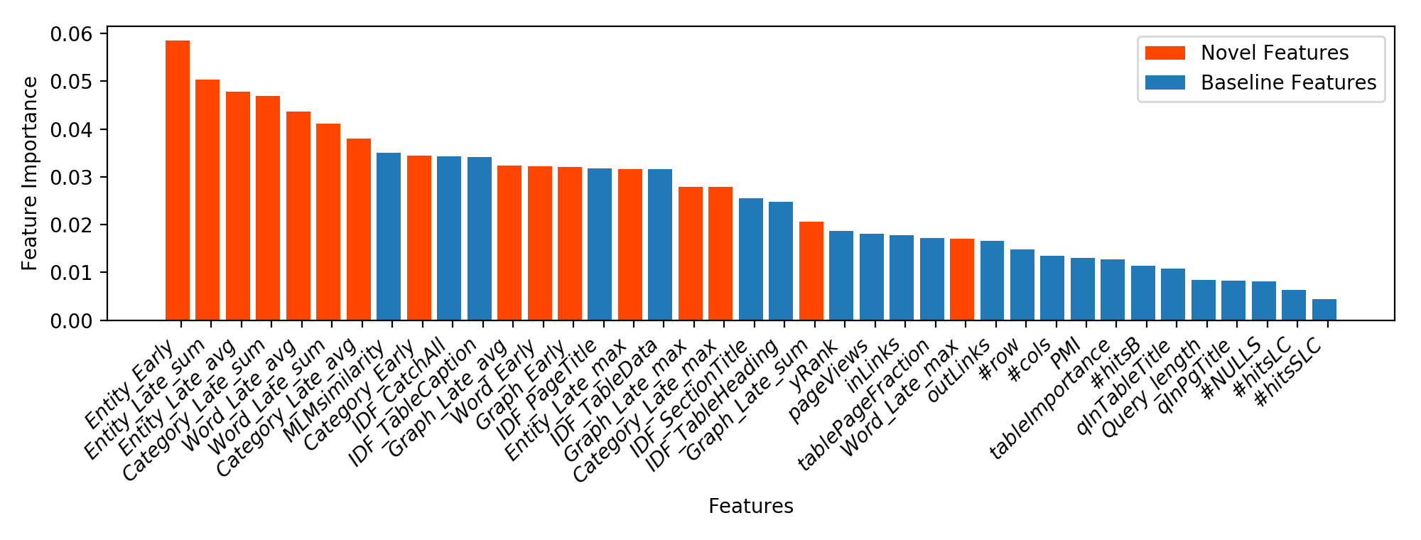
Figure 4 shows the importance of individual features for the table retrieval task, measured in terms of Gini importance. The novel features are distinguished by color. We observe that 8 out of the top 10 features are semantic features introduced in this paper.
5.5.2. Semantic Representations
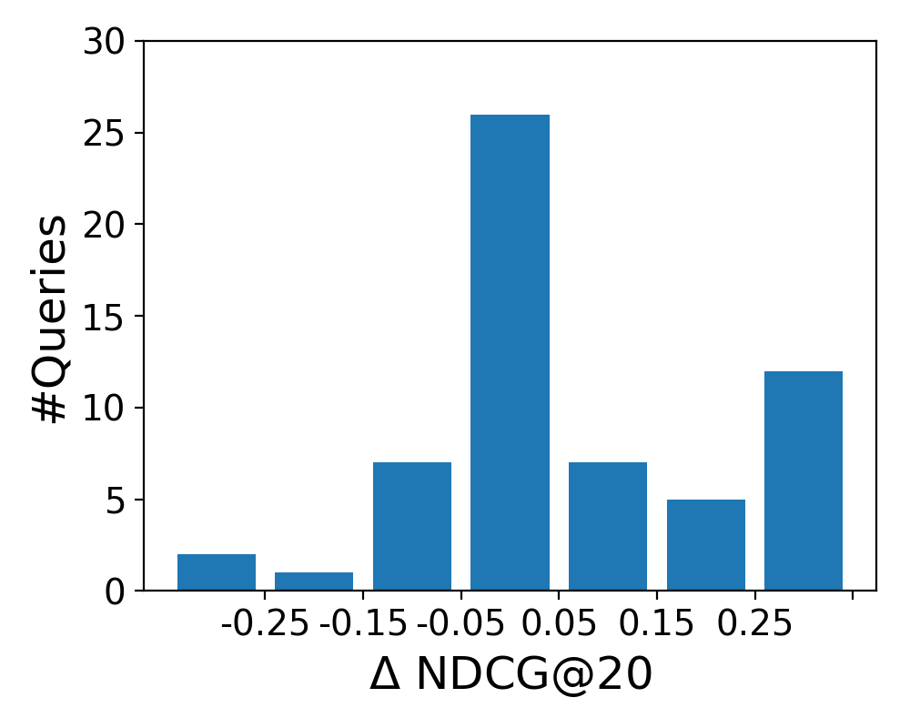
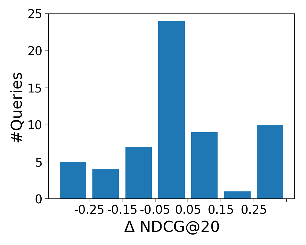
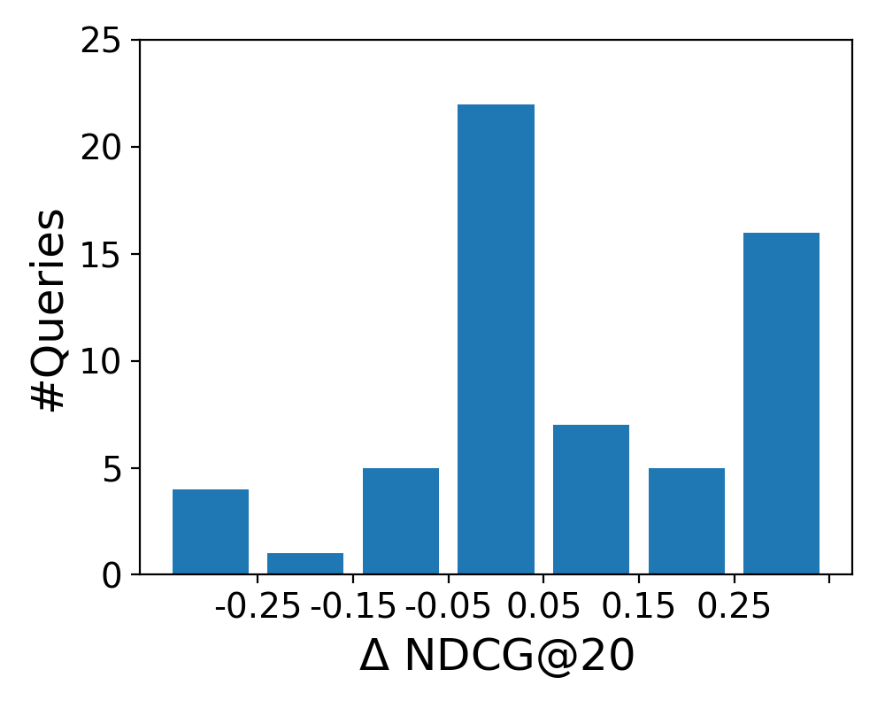
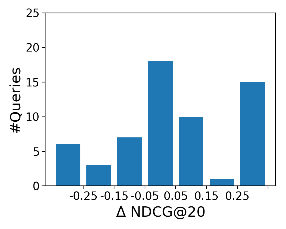
To analyze how the four semantic representations affect retrieval performance on the level of individual queries, we plot the difference between the LTR baseline and each semantic representation in Figure 5. The histograms show the distribution of queries according to NDCG@20 score difference (): the middle bar represents no change (0.05), while the leftmost and rightmost bars represents the number of queries that were hurt and helped substantially, respectively (0.25). We observe similar patterns for the bag-of-entities and word embeddings representations; the former has less queries that were significantly helped or hurt, while the overall improvement (over all topics) is larger. We further note the similarity of the shapes of the distributions for bag-of-categories and graph embeddings.
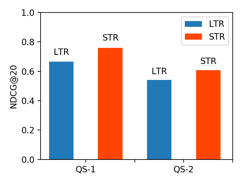
5.5.3. Query Subsets
On Figure 6, we plot the results for the LTR baseline and for our STR method according to the two query subsets, QS-1 and QS-2, in terms of NDCG@20. Generally, both methods perform better on QS-1 than on QS-2. This is mainly because QS-2 queries are more focused (each targeting a specific type of instance, with a required property), and thus are considered more difficult. Importantly, STR achieves consistent improvements over LTR on both query subsets.
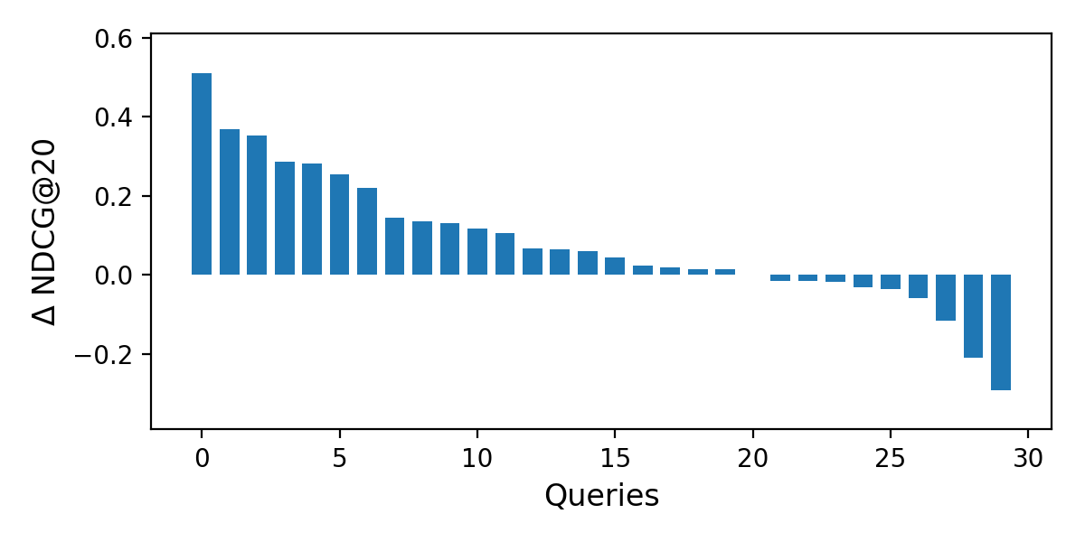
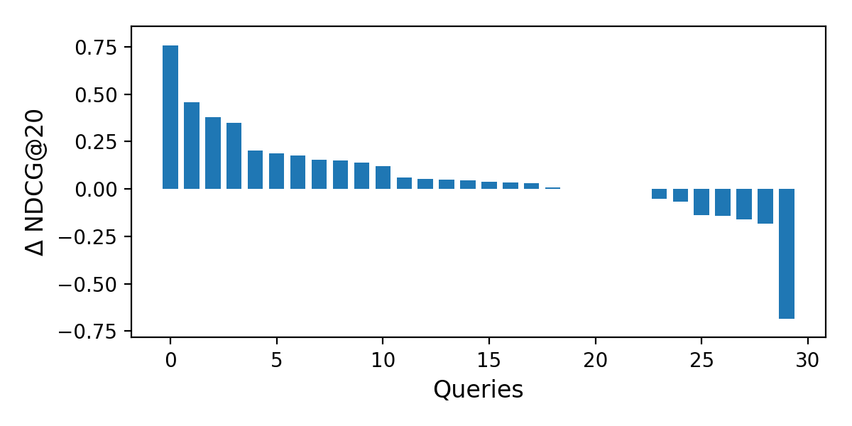
5.5.4. Individual Queries
We plot the difference between the LTR baseline and STR for the two query subsets in Figure 7. Table 7 lists the queries that we discuss below. The leftmost bar in Figure 7(a) corresponds to the query “stocks.” For this broad query, there are two relevant and one highly relevant tables. LTR does not retrieve any highly relevant tables in the top 20, while STR manages to return one highly relevant table in the top 10. The rightmost bar in Figure 7(a) corresponds to the query “ibanez guitars.” For this query, there are two relevant and one highly relevant tables. LTR produces an almost perfect ranking for this query, by returning the highly relevant table at the top rank, and the two relevant tables at ranks 2 and 4. STR returns a non-relevant table at the top rank, thereby pushing the relevant results down in the ranking by a single position, resulting in a decrease of 0.29 in NDCG@20.
The leftmost bar in Figure 7(b) corresponds to the query “board games number of players.” For this query, there are only two relevant tables according to the ground truth. STR managed to place them in the 1st and 3rd rank positions, while LTR returned only one of them at position 13th. The rightmost bar in Figure 7(b) is the query “cereals nutritional value.” Here, there is only one highly relevant result. LTR managed to place it in rank one, while it is ranked eighth by STR. Another interesting query is “irish counties area” (third bar from the left in Figure 7(b)), with three highly relevant and three relevant results according to the ground truth. LTR returned two highly relevant and one relevant results at ranks 1, 2, and 4. STR, on the other hand, placed the three highly relevant results in the top 3 positions and also returned the three relevant tables at positions 4, 6, and 7.
| Query | Rel | LTR | STR |
| QS-1-24: stocks | |||
| Stocks for the Long Run / Key Data Findings: annual real returns | 2 | - | 6 |
| TOPIX / TOPIX New Index Series | 1 | 9 | - |
| Hang Seng Index / Selection criteria for the HSI constituent stocks | 1 | - | - |
| QS-1-21: ibanez guitars | |||
| Ibanez / Serial numbers | 2 | 1 | 2 |
| Corey Taylor / Equipment | 1 | 2 | 3 |
| Fingerboard / Examples | 1 | 4 | 5 |
| QS-2-27: board games number of players | |||
| List of Japanese board games | 1 | 13 | 1 |
| List of licensed Risk game boards / Risk Legacy | 1 | - | 3 |
| QS-2-21: cereals nutritional value | |||
| Sesame / Sesame seed kernels, toasted | 2 | 1 | 8 |
| QS-2-20: irish counties area | |||
| Counties of Ireland / List of counties | 2 | 2 | 1 |
| List of Irish counties by area / See also | 2 | 1 | 2 |
| List of flags of Ireland / Counties of Ireland Flags | 2 | - | 3 |
| Provinces of Ireland / Demographics and politics | 1 | 4 | 4 |
| Toponymical list of counties of the United Kingdom / Northern … | 1 | - | 7 |
| Múscraige / Notes | 1 | - | 6 |
6. Related Work
There is an increasing amount of work on tables, addressing a wide range of tasks, including table search, table mining, table extension, and table completion. Table search is a fundamental problem on its own, as well as used often as a core component in other tasks.
Table Search
Users are likely to search for tables when they need structured or relational data. Cafarella et al. (2008b) pioneered the table search task by introducing the WebTables system. The basic idea is to fetch the top-ranked results returned by a web search engine in response to the query, and then extract the top- tables from those pages. Further refinements to the same idea are introduced in (Cafarella et al., 2009). Venetis et al. (2011) leverage a database of class labels and relationships extracted from the Web, which are attached to table columns, for recovering table semantics. This information is then used to enhance table search. Pimplikar and Sarawagi (2012) search for tables using column keywords, and match these keywords against the header, body, and context of tables. Google Web Tables222https://research.google.com/tables provides an example of a table search system interface; the developers’ experiences are summarized in (Balakrishnan et al., 2015). To enrich the diversity of search results, Nguyen et al. (2015) design a goodness measure for table search and selection. Apart from keyword-based search, tables may also be retrieved using a given “local” table as the query (Ahmadov et al., 2015; Das Sarma et al., 2012; Limaye et al., 2010). We are not aware of any work that performs semantic matching of tables against queries.
Table Extension/Completion
Table extension refers to the task of extending a table with additional elements, which are typically new columns (Das Sarma et al., 2012; Cafarella et al., 2009; Lehmberg et al., 2015; Yakout et al., 2012; Bhagavatula et al., 2013). These methods commonly use table search as the first step (Lehmberg et al., 2015; Bhagavatula et al., 2013; Yakout et al., 2012). Searching related tables is also used for row extension. In (Das Sarma et al., 2012), two tasks of entity complement and schema complement are addressed, to extend entity rows and columns respectively. Zhang and Balog (2017b) populate row and column headings of tables that have an entity focus. Table completion is the task of filling in empty cells within a table. Ahmadov et al. (2015) introduce a method to extract table values from related tables and/or to predict them using machine learning methods.
Table Mining
The abundance of information in tables has raised great interest in table mining research (Cafarella et al., 2011; Cafarella et al., 2008b; Madhavan et al., 2009; Sarawagi and Chakrabarti, 2014; Venetis et al., 2011; Zhang and Chakrabarti, 2013). Munoz et al. (2014) recover table semantics by extracting RDF triples from Wikipedia tables. Similarly, Cafarella et al. (2008b) mine table relations from a huge table corpus extracted from a Google crawl. Tables could also be searched to answer questions or mined to extend knowledge bases. Yin et al. (2016) take tables as a knowledge base to execute queries using deep neural networks. Sekhavat et al. (2014) augment an existing knowledge base (YAGO) with a probabilistic method by making use of table information. Similar work is carried out in (Dong et al., 2014), with tabular information used for knowledge base augmentation. Another line of work concerns table annotation and classification. Zwicklbauer et al. (2013) introduce a method to annotate table headers by mining column content. Crestan and Pantel (2011) introduce a supervised framework for classifying HTML tables into a taxonomy by examining the contents of a large number of tables. Apart from all the mentioned methods above, table mining also includes tasks like table interpretation (Cafarella et al., 2008b; Munoz et al., 2014; Venetis et al., 2011) and table recognition (Crestan and Pantel, 2011; Zwicklbauer et al., 2013). In the problem space of table mining, table search is an essential component.
7. Conclusion
In this paper, we have introduced and addressed the problem of ad hoc table retrieval: answering a keyword query with a ranked list of tables. We have developed a novel semantic matching framework, where queries and tables can be represented using semantic concepts (bag-of-entities and bag-of-categories) as well as continuous dense vectors (word and graph embeddings) in a uniform way. We have introduced multiple similarity measures for matching those semantic representations. For evaluation, we have used a purpose-built test collection based on Wikipedia tables. Finally, we have demonstrated substantial and significant improvements over a strong baseline. In future work, we wish to relax our requirements regarding the focus on Wikipedia tables, and make our methods applicable to other types of tables, like scientific tables (Gao and Callan, 2017) or Web tables.
References
- (1)
- Ahmadov et al. (2015) Ahmad Ahmadov, Maik Thiele, Julian Eberius, Wolfgang Lehner, and Robert Wrembel. 2015. Towards a Hybrid Imputation Approach Using Web Tables.. In Proc. of BDC ’15. 21–30.
- Balakrishnan et al. (2015) Sreeram Balakrishnan, Alon Y. Halevy, Boulos Harb, Hongrae Lee, Jayant Madhavan, Afshin Rostamizadeh, Warren Shen, Kenneth Wilder, Fei Wu, and Cong Yu. 2015. Applying WebTables in Practice. In Proc. of CIDR ’15.
- Balog et al. (2011) Krisztian Balog, Marc Bron, and Maarten De Rijke. 2011. Query modeling for entity search based on terms, categories, and examples. ACM Trans. Inf. Syst. 29, 4, Article 22 (Dec. 2011), 22:1–22:31 pages.
- Bhagavatula et al. (2013) Chandra Sekhar Bhagavatula, Thanapon Noraset, and Doug Downey. 2013. Methods for Exploring and Mining Tables on Wikipedia. In Proc. of IDEA ’13. 18–26.
- Bhagavatula et al. (2015) Chandra Sekhar Bhagavatula, Thanapon Noraset, and Doug Downey. 2015. TabEL: Entity Linking in Web Tables. In Proc. of ISWC ’15. 425–441.
- Cafarella et al. (2009) Michael J. Cafarella, Alon Halevy, and Nodira Khoussainova. 2009. Data Integration for the Relational Web. Proc. of VLDB Endow. 2 (2009), 1090–1101.
- Cafarella et al. (2011) Michael J. Cafarella, Alon Halevy, and Jayant Madhavan. 2011. Structured Data on the Web. Commun. ACM 54 (2011), 72–79.
- Cafarella et al. (2008a) Michael J. Cafarella, Alon Halevy, Daisy Zhe Wang, Eugene Wu, and Yang Zhang. 2008a. Uncovering the Relational Web. In Proc. of WebDB ’08.
- Cafarella et al. (2008b) Michael J. Cafarella, Alon Halevy, Daisy Zhe Wang, Eugene Wu, and Yang Zhang. 2008b. WebTables: Exploring the Power of Tables on the Web. Proc. of VLDB Endow. 1 (2008), 538–549.
- Chen et al. (2016) Jing Chen, Chenyan Xiong, and Jamie Callan. 2016. An Empirical Study of Learning to Rank for Entity Search. In Proc. of SIGIR ’16. 737–740.
- Crestan and Pantel (2011) Eric Crestan and Patrick Pantel. 2011. Web-scale Table Census and Classification. In Proc. of WSDM ’11. 545–554.
- Das Sarma et al. (2012) Anish Das Sarma, Lujun Fang, Nitin Gupta, Alon Halevy, Hongrae Lee, Fei Wu, Reynold Xin, and Cong Yu. 2012. Finding Related Tables. In Proc. of SIGMOD ’12. 817–828.
- Dong et al. (2014) Xin Dong, Evgeniy Gabrilovich, Geremy Heitz, Wilko Horn, Ni Lao, Kevin Murphy, Thomas Strohmann, Shaohua Sun, and Wei Zhang. 2014. Knowledge Vault: A Web-scale Approach to Probabilistic Knowledge Fusion. In Proc. of KDD ’14. 601–610.
- Fleiss et al. (1971) J.L. Fleiss and others. 1971. Measuring nominal scale agreement among many raters. Psychological Bulletin 76 (1971), 378–382.
- Ganguly et al. (2015) Debasis Ganguly, Dwaipayan Roy, Mandar Mitra, and Gareth J.F. Jones. 2015. Word Embedding Based Generalized Language Model for Information Retrieval. In Proc. of SIGIR ’15. 795–798.
- Gao and Callan (2017) Kyle Yingkai Gao and Jamie Callan. 2017. Scientific Table Search Using Keyword Queries. CoRR abs/1707.03423 (2017).
- Grbovic et al. (2015) Mihajlo Grbovic, Nemanja Djuric, Vladan Radosavljevic, Fabrizio Silvestri, and Narayan Bhamidipati. 2015. Context- and Content-aware Embeddings for Query Rewriting in Sponsored Search. In Proc. of SIGIR ’15. 383–392.
- Hasibi et al. (2017a) Faegheh Hasibi, Krisztian Balog, Darío Garigliotti, and Shuo Zhang. 2017a. Nordlys: A Toolkit for Entity-Oriented and Semantic Search. In Proceedings of SIGIR ’17. 1289–1292.
- Hasibi et al. (2017b) Faegheh Hasibi, Fedor Nikolaev, Chenyan Xiong, Krisztian Balog, Svein Erik Bratsberg, Alexander Kotov, and Jamie Callan. 2017b. DBpedia-Entity V2: A Test Collection for Entity Search. In Proc. of SIGIR ’17. 1265–1268.
- Kenter and de Rijke (2015) Tom Kenter and Maarten de Rijke. 2015. Short Text Similarity with Word Embeddings. In Proc. of CIKM ’15. 1411–1420.
- Lehmberg et al. (2015) Oliver Lehmberg, Dominique Ritze, Petar Ristoski, Robert Meusel, Heiko Paulheim, and Christian Bizer. 2015. The Mannheim Search Join Engine. Web Semant. 35 (2015), 159–166.
- Limaye et al. (2010) Girija Limaye, Sunita Sarawagi, and Soumen Chakrabarti. 2010. Annotating and Searching Web Tables Using Entities, Types and Relationships. Proc. of VLDB Endow. 3 (2010), 1338–1347.
- Liu (2011) Tie-Yan Liu. 2011. Learning to Rank for Information Retrieval. Springer Berlin Heidelberg.
- Macdonald et al. (2012) Craig Macdonald, Rodrygo L T Santos, and Iadh Ounis. 2012. On the Usefulness of Query Features for Learning to Rank. In Proc. of CIKM ’12. 2559–2562.
- Madhavan et al. (2009) Jayant Madhavan, Loredana Afanasiev, Lyublena Antova, and Alon Y. Halevy. 2009. Harnessing the Deep Web: Present and Future. CoRR abs/0909.1785 (2009).
- Manotumruksa et al. (2016) Jarana Manotumruksa, Craig MacDonald, and Iadh Ounis. 2016. Modelling User Preferences using Word Embeddings for Context-Aware Venue Recommendation. CoRR abs/1606.07828 (2016).
- Mikolov et al. (2013) Tomas Mikolov, Ilya Sutskever, Kai Chen, Greg Corrado, and Jeffrey Dean. 2013. Distributed Representations of Words and Phrases and Their Compositionality. In Proc. of NIPS ’13. 3111–3119.
- Mitra et al. (2016) Bhaskar Mitra, Eric T. Nalisnick, Nick Craswell, and Rich Caruana. 2016. A Dual Embedding Space Model for Document Ranking. CoRR abs/1602.01137 (2016).
- Munoz et al. (2014) Emir Munoz, Aidan Hogan, and Alessandra Mileo. 2014. Using Linked Data to Mine RDF from Wikipedia’s Tables. In Proc. of WSDM ’14. 533–542.
- Nguyen et al. (2015) Thanh Tam Nguyen, Quoc Viet Hung Nguyen, Weidlich Matthias, and Aberer Karl. 2015. Result Selection and Summarization for Web Table Search. In ISDE ’15. 231–242.
- Ogilvie and Callan (2003) Paul Ogilvie and Jamie Callan. 2003. Combining Document Representations for Known-item Search. In Proc. of SIGIR ’03. 143–150.
- Pennington et al. (2014) Jeffrey Pennington, Richard Socher, and Christopher D Manning. 2014. GloVe: Global Vectors for Word Representation. In Proc. of EMNLP ’14. 1532–1543.
- Perozzi et al. (2014) Bryan Perozzi, Rami Al-Rfou, and Steven Skiena. 2014. DeepWalk: Online Learning of Social Representations. In Proc. of KDD ’14. 701–710.
- Pimplikar and Sarawagi (2012) Rakesh Pimplikar and Sunita Sarawagi. 2012. Answering Table Queries on the Web Using Column Keywords. Proc. of VLDB Endow. 5 (2012), 908–919.
- Qin et al. (2010) Tao Qin, Tie-Yan Liu, Jun Xu, and Hang Li. 2010. LETOR: A Benchmark Collection for Research on Learning to Rank for Information Retrieval. Inf. Retr. 13, 4 (Aug 2010), 346–374.
- Raviv et al. (2016) Hadas Raviv, Oren Kurland, and David Carmel. 2016. Document Retrieval Using Entity-Based Language Models. In Proc. of SIGIR ’16. 65–74.
- Ristoski and Paulheim (2016) Petar Ristoski and Heiko Paulheim. 2016. RDF2vec: RDF Graph Embeddings for Data Mining. In Proc. of ISWC ’16. 498–514.
- Sarawagi and Chakrabarti (2014) Sunita Sarawagi and Soumen Chakrabarti. 2014. Open-domain Quantity Queries on Web Tables: Annotation, Response, and Consensus Models. In Proc. of KDD ’14. 711–720.
- Sekhavat et al. (2014) Yoones A. Sekhavat, Francesco Di Paolo, Denilson Barbosa, and Paolo Merialdo. 2014. Knowledge Base Augmentation using Tabular Data. In Proc. of LDOW ’14.
- Tang et al. (2015) Jian Tang, Meng Qu, Mingzhe Wang, Ming Zhang, Jun Yan, and Qiaozhu Mei. 2015. LINE: Large-scale Information Network Embedding. In Proc. of WWW ’15. 1067–1077.
- Tyree et al. (2011) Stephen Tyree, Kilian Q Weinberger, Kunal Agrawal, and Jennifer Paykin. 2011. Parallel Boosted Regression Trees for Web Search Ranking. In Proc. of WWW ’11. 387–396.
- Venetis et al. (2011) Petros Venetis, Alon Halevy, Jayant Madhavan, Marius Paşca, Warren Shen, Fei Wu, Gengxin Miao, and Chung Wu. 2011. Recovering Semantics of Tables on the Web. Proc. of VLDB Endow. 4 (2011), 528–538.
- Vulić and Moens (2015) Ivan Vulić and Marie-Francine Moens. 2015. Monolingual and Cross-Lingual Information Retrieval Models Based on (Bilingual) Word Embeddings. In Proc. of SIGIR ’15. 363–372.
- Xiong et al. (2017) Chenyan Xiong, Jamie Callan, and Tie-Yan Liu. 2017. Word-Entity Duet Representations for Document Ranking. In Proc. of SIGIR ’17. 763–772.
- Yakout et al. (2012) Mohamed Yakout, Kris Ganjam, Kaushik Chakrabarti, and Surajit Chaudhuri. 2012. InfoGather: Entity Augmentation and Attribute Discovery by Holistic Matching with Web Tables. In Proc. of SIGMOD ’12. 97–108.
- Yin et al. (2016) Pengcheng Yin, Zhengdong Lu, Hang Li, and Ben Kao. 2016. Neural Enquirer: Learning to Query Tables in Natural Language. In Proc. of IJCAI ’16. 2308–2314.
- Zhang and Chakrabarti (2013) Meihui Zhang and Kaushik Chakrabarti. 2013. InfoGather+: Semantic Matching and Annotation of Numeric and Time-varying Attributes in Web Tables. In Proc. of SIGMOD ’13. 145–156.
- Zhang and Balog (2017a) Shuo Zhang and Krisztian Balog. 2017a. Design Patterns for Fusion-Based Object Retrieval. In Proc. of ECIR ’17. 684–690.
- Zhang and Balog (2017b) Shuo Zhang and Krisztian Balog. 2017b. EntiTables: Smart Assistance for Entity-Focused Tables. In Proc. of SIGIR ’17. 255–264.
- Zhou et al. (2015) Guangyou Zhou, Tingting He, Jun Zhao, and Po Hu. 2015. Learning Continuous Word Embedding with Metadata for Question Retrieval in Community Question Answering. In Proc. of ACL ’15. 250–259.
- Zwicklbauer et al. (2013) Stefan Zwicklbauer, Christoph Einsiedler, Michael Granitzer, and Christin Seifert. 2013. Towards Disambiguating Web Tables. In Proc. of ISWC-PD ’13. 205–208.