AdaK-NER: An Adaptive Top- $\mathbf{K}$ Approach
for Named Entity Recognition with Incomplete Annotations

Hongtao Ruan¹ Liying Zheng²&Peixian Hu³

Abstract

State-of-the-art Named Entity Recognition (NER) models rely heavily on large amounts of fully annotated training data. However, accessible data are often incompletely annotated in the industry like Financial Technology. Normally the unannotated tokens are regarded as non-entities by default, while we underline that these tokens could either be non-entities or part of any entity. Here, we study NER modeling with incomplete annotated data where only a fraction of the named entities are labeled, and the unlabeled tokens are equivalently multi-labeled by every possible label. Taking multi-labeled tokens into account, the numerous possible paths can distract the training model from the gold path (ground truth label sequence), and thus hinders the learning ability. In this paper, we propose AdaK-NER, named the adaptive top- $K$ approach, to help the model focus on a smaller feasible region where the gold path is more likely to be located. We demonstrate the superiority of our approach through extensive experiments on both English and Chinese datasets, averagely improving $2\%$ in F-score on the CoNLL-2003 and over $10\%$ on two Chinese datasets from Financial Technology compared with the prior state-of-the-art works.

1 Introduction

Named Entity Recognition (NER) Li et al. (2020); Sang and De Meulder (2003); Peng et al. (2019) is a fundamental task in Natural Language Processing (NLP). NER task aims at recognizing the meaningful entities occurring in the text, which can benefit various downstream tasks, such as question answering Cao et al. (2019), event extraction Wei et al. (2020), and opinion mining Poria et al. (2016). Especially, by detecting relevant entities in Financial Technology, NER helps financial professionals efficiently leverage the information of news, which is paramount in making high-quality decisions.

Strides in statistical models, such as Conditional Random Field (CRF) Lafferty et al. (2001) and pre-trained language models like BERT Devlin et al. (2018), have equipped NER with new learning principles Li et al. (2020). Pre-trained model with rich representation ability can discover hidden features automatically while CRF can capture the dependencies between labels with the BIO or BIOES tagging scheme.

However, most existing methods rely on large amounts of fully annotated information for training NER models Li et al. (2020); Jia et al. (2020). Fulfilling such requirements is expensive and laborious in the industry like Financial Technology. Annotators, are not likely to be fully equipped with comprehensive domain knowledge, only annotate the named entities they recognize and let the others off, resulting in incomplete annotations. They typically do not specify the non-entity Surdeanu et al. (2010), so that the recognized entities are the only available annotations. Figure 1(a) shows examples of both gold path¹¹1A path is a label sequence for a given sentence. and incomplete path.

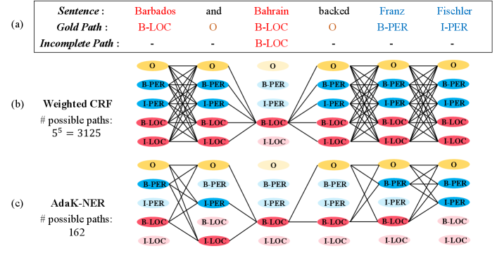
Refer to caption — Figure 1: (a) The sentence is annotated with BIO tagging scheme. The entity types are person (PER) and location (LOC). Only the entity ‘Bahrain’ of LOC is recognized, while ‘Barbados’ of LOC and ‘Franz Fischler’ of PER are missing. (b) Weighted CRF model considers all the $3125$ possible paths with $5$ unannotated tokens for $q$ estimation. (c) In our model, we build a candidate mask to filter out the less likely labels (labels in faded color). Therefore, the possible paths of our model is significantly less than weighted CRF.

For corpus with incomplete annotations, each unannotated token can either be part of an entity or non-entity, making the token equivalently multi-labeled by every possible label. Since conventional CRF algorithms require fully annotated sentences, a strand of literature suggests assigning weights to possible labels Shang et al. (2018); Jie et al. (2019). Fuzzy CRF Shang et al. (2018) focused on filling the unannotated tokens by assigning equal probability to every possible path. Further, Jie Jie et al. (2019) introduced a weighted CRF method to seek a more reasonable distribution $q$ for all possible paths, attempting to pay more attention to those paths with high potential to be gold path.

Ideally, through comprehensive learning on $q$ distribution, the gold path can be correctly discovered. However, this perfect situation is difficult to achieve in practical applications. Intuitively, taking all possible paths into consideration will distract the model from the gold path, as the feasible region (the set of possible paths where we search for the gold path) grows exponentially with the length of the unannotated tokens increasing, which might cause failure to identify the gold path.

To address this issue, one promising direction is to prune the size of feasible region during training. We assume the unknown gold path is among or very close to the top- $K$ paths with the highest possibilities. Specifically, we utilize a novel adaptive $K$ -best loss to help the training model focus on a smaller feasible region where the gold path is likely to be located. Furthermore, once a path is identified as a disqualified sequence, it will be removed from the feasible region. This operation can thus drastically eliminate redundancy without undermining the effectiveness. For this purpose, a candidate mask is built to filter out the less likely paths, so as to restrict the size of the feasible region.

Trained in this way, our AdaK-NER overcomes the shortcomings of Fuzzy CRF and weighted CRF, resulting in a significant improvement on both precision and recall, and a higher $F_{1}$ score as well.

In summary, the contributions of this work are:

•

We present a $K$ -best mechanism for improving incomplete annotated NER, aiming to focus on the gold path effectively from the most possible candidates.
•

We demonstrate both qualitatively and quantitatively that our approach achieves state-of-the-art performance compared to various baselines on both English and Chinese datasets.

2 Proposed Approach

Let ${\boldsymbol{x}}=({\boldsymbol{x}}_{1},{\boldsymbol{x}}_{2},\cdots,{\boldsymbol{x}}_{n})$ be a training sentence of length $n$ , token ${\boldsymbol{x}}_{i}\in{\boldsymbol{X}}$ . Correspondingly, ${\boldsymbol{y}}=({\boldsymbol{y}}_{1},{\boldsymbol{y}}_{2},\cdots,{\boldsymbol{y}}_{n})$ denotes the complete label sequence, ${\boldsymbol{y}}_{i}\in{\boldsymbol{Y}}$ . The NER problem can be defined as inferring ${\boldsymbol{y}}$ based on ${\boldsymbol{x}}$ .

Under the incomplete annotation framework, we introduce the following terminologies. A possible path refers to a possible complete label sequence consistent with the annotated tokens. For example, a possible incomplete annotated label sequence for ${\boldsymbol{x}}$ can be ${\boldsymbol{y}}_{u}=(-,{\boldsymbol{y}}_{2},-,\cdots,-)$ , where token ${\boldsymbol{x}}_{2}$ is annotated as ${\boldsymbol{y}}_{2}$ and other missing labels are labeled as $-$ . ${\boldsymbol{y}}_{c}=({\boldsymbol{y}}_{c_{1}},{\boldsymbol{y}}_{2},\cdots,{\boldsymbol{y}}_{c_{n}})$ with ${\boldsymbol{y}}_{c_{i}}\in{\boldsymbol{Y}}$ , is a possible path for ${\boldsymbol{x}}$ , where all the missing labels $-$ are replaced by some elements in ${\boldsymbol{Y}}$ . Set $C({\boldsymbol{y}}_{u})$ denotes all possible complete paths for ${\boldsymbol{x}}$ with incomplete annotation ${\boldsymbol{y}}_{u}$ . $D=\{({\boldsymbol{x}}^{i},{\boldsymbol{y}}^{i}_{u})\}$ is the available incompletely annotated dataset.

For NER task, CRF Lafferty et al. (2001) is a traditional approach to capture the dependencies between the labels by modeling the conditional probability $p_{\boldsymbol{w}}({\boldsymbol{y}}|{\boldsymbol{x}})$ of a label sequence ${\boldsymbol{y}}$ given an input sequence ${\boldsymbol{x}}$ of length $n$ as:

p_{\boldsymbol{w}}({\boldsymbol{y}}|{\boldsymbol{x}})=\frac{\exp({\boldsymbol{w}}\cdot\Phi({\boldsymbol{x}},{\boldsymbol{y}}))}{\sum_{{\boldsymbol{y}}\in{\boldsymbol{Y}}^{n}}\exp({\boldsymbol{w}}\cdot\Phi({\boldsymbol{x}},{\boldsymbol{y}}))}.

(1)

$\Phi({\boldsymbol{x}},{\boldsymbol{y}})$ denotes the map from a pair of ${\boldsymbol{x}}$ and ${\boldsymbol{y}}$ to an arbitrary feature vector, ${\boldsymbol{w}}$ is the model parameter, $p_{\boldsymbol{w}}({\boldsymbol{y}}|{\boldsymbol{x}})$ is the probability of ${\boldsymbol{y}}$ predicted by the model. Once ${\boldsymbol{w}}$ has been estimated via minimizing negative log-likelihood:

L({\boldsymbol{w}},{\boldsymbol{x}})=-\log p_{\boldsymbol{w}}({\boldsymbol{y}}|{\boldsymbol{x}}),

(2)

the label sequence can be inferred by:

\hat{{\boldsymbol{y}}}=\arg\max_{{\boldsymbol{y}}\in{\boldsymbol{Y}}^{n}}p_{\boldsymbol{w}}({\boldsymbol{y}}|{\boldsymbol{x}}).\vspace{-1pt}

(3)

The original CRF learning algorithm requires a fully annotated sequence ${\boldsymbol{y}}$ , thus the incompletely annotated data is not directly applicable to it. Jie Jie et al. (2019) modified the loss function as follows:

L({\boldsymbol{w}},{\boldsymbol{x}})=-\log\sum_{{\boldsymbol{y}}\in C({\boldsymbol{y}}_{u})}q({\boldsymbol{y}}|{\boldsymbol{x}})p_{\boldsymbol{w}}({\boldsymbol{y}}|{\boldsymbol{x}}),\vspace{-1pt}

(4)

where $q({\boldsymbol{y}}|{\boldsymbol{x}})$ is an estimated distribution of all possible complete paths ${\boldsymbol{y}}\in C({\boldsymbol{y}}_{u})$ for ${\boldsymbol{x}}$ .

We illustrate their model in (Figure 1b). Note that when $q$ is a uniform distribution, the above CRF model is Fuzzy CRF Shang et al. (2018) which puts equal probability to all possible paths in $C({\boldsymbol{y}}_{u})$ . Jie Jie et al. (2019) claimed that $q$ should be highly skewed rather than uniformly distributed, therefore they presented a $k$ -fold cross-validation stacking method to approximate distribution $q$ .

Nonetheless, as Figure 1(b) shows, a sentence with only $6$ words ( $1$ annotated, $5$ unannotated) have $3125$ possible paths. We argued that identifying the gold path from all possible paths is like looking for a needle in a haystack. This motivates us to reduce redundant paths during training. We propose two major strategies (adaptive $K$ -best loss and candidate mask) to induce the model to focus on the gold path (Figure 1(c)), and two minor strategies (annealing technique and iterative sample selection) to further improve the model effectiveness in NER task. The workflow is summarized in Algorithm 1.

2.1 Adaptive $K$ -best Loss

Viterbi decoding algorithm is a dynamic programming technique to find the most possible path with only linear complexity, thus it could be used to predict a path for an input based on the parameters provided by the NER model. $K$ -best Viterbi decoding Huang and Chiang (2005) extends the original Viterbi decoding algorithm to extract the top- $K$ paths with the highest probabilities. In the incomplete data, the gold path is unknown. We hypothesize it is very likely to be the same with or close to one of the top- $K$ paths. This inspires us to introduce an auxiliary $K$ -best loss component to help the model focus on a smaller yet promising region. Weight is added to balance the weighted CRF loss and the auxiliary loss, and thus we modify (4) into:

	$\displaystyle L_{k}({\boldsymbol{w}},{\boldsymbol{x}})=$	$\displaystyle-(1-\lambda)\log\sum_{{\boldsymbol{y}}\in C({\boldsymbol{y}}_{u})}q({\boldsymbol{y}}\|{\boldsymbol{x}})p_{\boldsymbol{w}}({\boldsymbol{y}}\|{\boldsymbol{x}})$		(5)
		$\displaystyle-\lambda\log\sum_{{\boldsymbol{y}}\in K_{\boldsymbol{w}}(x)}p_{w}({\boldsymbol{y}}\|{\boldsymbol{x}}),$		(5)

where $K_{\boldsymbol{w}}({\boldsymbol{x}})$ represents the top- $K$ paths decoded by constrained $K$ -best Viterbi algorithm²²2The constrained decoding ensures the resulting complete paths are compatible with the incomplete annotations. with parameters ${\boldsymbol{w}}$ , and $\lambda$ is an adaptive weight coefficient.

2.2 Estimating $q$ with Candidate Mask

We divide the training data into $k$ folds and employ $k$ -fold cross-validation stacking to estimate $q$ for each hold-out fold Jie et al. (2019). We propose an interpolation mode to adjust $q$ by increasing the probabilities for paths with high confidence and decreasing for the others. The probability of each possible path is a temperature softmax of $\log p_{{\boldsymbol{w}}_{i}}$ :

\displaystyle q_{{\boldsymbol{w}}_{i}}({\boldsymbol{y}}|{\boldsymbol{x}})=\frac{\exp\left(\log p_{{\boldsymbol{w}}_{i}}({\boldsymbol{y}}|{\boldsymbol{x}})/T\right)}{\sum_{{\boldsymbol{y}}}\exp\left(\log p_{{\boldsymbol{w}}_{i}}({\boldsymbol{y}}|{\boldsymbol{x}})/T\right)},

(6)

where $T>0$ denotes the temperature and ${\boldsymbol{w}}_{i}$ is the model trained by holding out the $i$ -th fold. A higher temperature produces a softer probability distribution over the paths, resulting in more diversity and also more mistakes Hinton et al. (2015). We iterate the cross-validation until $q$ converges.

Jie Jie et al. (2019) estimated $q({\boldsymbol{y}}|{\boldsymbol{x}})$ for each ${\boldsymbol{y}}\in C({\boldsymbol{y}}_{u})$ while the size of $C({\boldsymbol{y}}_{u})$ grows exponentially on the number of unannotated tokens in ${\boldsymbol{x}}$ . To reduce the number of possible paths for $q$ estimation, we build candidate mask based on the $K$ -best candidates and the self-built candidates.

Data:

D=\{({\boldsymbol{x}}^{i},{\boldsymbol{y}}_{u}^{i})\}

Randomly divide

D

into

k

folds:

D_{1},D_{2},\cdots,D_{k}

Entity Dictionary

\mathcal{H}\leftarrow\emptyset

Initialize model

M

with parameters

\hat{{\boldsymbol{w}}}

Initialize

q

distributions {

q(\cdot|{\boldsymbol{x}}^{i})

}

Sample importance score

s_{i}\leftarrow 1

hyper-parameters

s

and

c

for iteration = $1,\cdots,N$ do

% Sample Selection

D^{{}^{\prime}}\leftarrow D

for j = $1,\cdots,k$ do

D_{j}^{{}^{\prime}}\leftarrow D_{j}

for $({\boldsymbol{x}}^{i},{\boldsymbol{y}}_{u}^{i})\in D_{j}^{{}^{\prime}}$ do

if $s_{i}<s$ then

remove

({\boldsymbol{x}}^{i},{\boldsymbol{y}}_{u}^{i})

from

D_{j}^{{}^{\prime}}

and

D^{{}^{\prime}}

end if

end for

q

Distribution Estimating

for j = $1,\cdots,k$ do

Train

M({\boldsymbol{w}}_{j})

D^{{}^{\prime}}\backslash D_{j}^{{}^{\prime}}

: Eq.(7)

for $({\boldsymbol{x}}^{i},{\boldsymbol{y}}_{u}^{i})\in D_{j}^{{}^{\prime}}$ do

Predict

K_{b}({\boldsymbol{x}}^{i})

M(\hat{{\boldsymbol{w}}})

Extract

H({\boldsymbol{x}}^{i})

\mathcal{H}

Possible paths

S=S({\boldsymbol{y}}_{u}^{i},K_{b}({\boldsymbol{x}}^{i}),H({\boldsymbol{x}}^{i}))

Estimate

q({\boldsymbol{y}}|{\boldsymbol{x}}^{i})

for

{\boldsymbol{y}}\in S

: Eq.(6)

s_{i}=\max_{\boldsymbol{y}}p_{{\boldsymbol{w}}_{j}}({\boldsymbol{y}}|{\boldsymbol{x}}^{i})

e_{i}\leftarrow

{

entities

} predicted by

M({\boldsymbol{w}}_{j})

end for

% Dictionary

\mathcal{H}

Updating

\mathcal{H}\leftarrow\emptyset

for $entity\in\cup e_{i}$ do

if $entity\notin\mathcal{H}$ and $freq(entity)$ > $c$ then

\mathcal{H}\leftarrow add\_entity(\mathcal{H},entity)

end if

end for

Train

M({\boldsymbol{w}}^{\prime})

D

with

q

: Eq.(7)

if $F_{1}$ of $M({\boldsymbol{w}}^{\prime})>F_{1}$ of $M(\hat{{\boldsymbol{w}}})$ on Dev then

\hat{{\boldsymbol{w}}}\leftarrow{\boldsymbol{w}}^{\prime}

end if

end for

Return the final NER model

M(\hat{{\boldsymbol{w}}})

Algorithm 1 AdaK-NER

$K$ -best Candidates.

During the end of each iteration, we train a model $M(\hat{{\boldsymbol{w}}})$ on the whole training data $D$ . In the next iteration, we use the trained model $M(\hat{{\boldsymbol{w}}})$ to identify $K$ -best candidates set $K_{b}({\boldsymbol{x}})$ for each sample ${\boldsymbol{x}}$ by constrained $K$ -best Viterbi decoding. $K_{b}({\boldsymbol{x}})=\{\hat{K}_{i}({\boldsymbol{x}})\}_{i=1,\cdots,K}$ contains top- $K$ possible paths with the highest probabilities, where $\hat{K}_{i}({\boldsymbol{x}})=[\hat{K}_{i}({\boldsymbol{x}}_{1}),\hat{K}_{i}({\boldsymbol{x}}_{2}),\cdots,\hat{K}_{i}({\boldsymbol{x}}_{n})]$ .

Self-built Candidates.

In the current iteration, after training a model $M({\boldsymbol{w}}_{i})$ on $(k-1)$ folds, we use $M({\boldsymbol{w}}_{i})$ to predict a path for each sample in the hold-out fold, and extract entities from the predicted path. Then we merge all entities identified by $k$ models $\{M({\boldsymbol{w}}_{i})\}_{i=1,\cdots,k}$ , resulting an entity dictionary $\mathcal{H}$ . For each sample ${\boldsymbol{x}}$ we conjecture that its named entities should lie in the dictionary $\mathcal{H}$ . Consequently, in the next iteration we form a self-built candidate $H({\boldsymbol{x}})=[H({\boldsymbol{x}}_{1}),H({\boldsymbol{x}}_{2}),\cdots,H({\boldsymbol{x}}_{n})]$ for each ${\boldsymbol{x}}$ of length $n$ . $H({\boldsymbol{x}}_{j})$ is the corresponding entity label if the token ${\boldsymbol{x}}_{j}$ is part of an entity in $\mathcal{H}$ , otherwise $H({\boldsymbol{x}}_{j})$ is O label.

We utilize the above candidates (i.e., the $K$ -best candidates set $K_{b}({\boldsymbol{x}})$ and the self-built candidate $H({\boldsymbol{x}})$ ) to construct a candidate mask for ${\boldsymbol{x}}$ . For each unannotated ${\boldsymbol{x}}_{j}$ in ${\boldsymbol{x}}$ , the possible label set consists of (1) O label (2) $H({\boldsymbol{x}}_{j})$ , (3) $\cup_{i=1}^{K}\hat{K}_{i}({\boldsymbol{x}}_{j})$ .

For example, as Figure 1(c) shows, the unannotated token ‘Barbados’ is predicted as B-PER and B-LOC in the above candidate paths, we treat B-PER, B-LOC and O label as the possible labels of ‘Barbados’ and mask the other labels.

With this masking scheme, we can significantly narrow down the feasible region of ${\boldsymbol{x}}$ (Figure 1(c)) when estimating $q(\cdot|{\boldsymbol{x}})$ . After estimating $q(\cdot|{\boldsymbol{x}})$ , we can train a model through the modified loss:

	$\displaystyle L_{m}({\boldsymbol{w}},{\boldsymbol{x}})=$	$\displaystyle-(1-\lambda)\log\sum_{{\boldsymbol{y}}\in S}q({\boldsymbol{y}}\|{\boldsymbol{x}})p_{\boldsymbol{w}}({\boldsymbol{y}}\|{\boldsymbol{x}})$		(7)
		$\displaystyle-\lambda\log\sum_{{\boldsymbol{y}}\in K_{\boldsymbol{w}}({\boldsymbol{x}})}p_{\boldsymbol{w}}({\boldsymbol{y}}\|{\boldsymbol{x}}),$		(7)

where $S=S({\boldsymbol{y}}_{u},K_{b}({\boldsymbol{x}}),H({\boldsymbol{x}}))$ contains the possible paths restricted by the candidate mask.

Dataset	Train		Dev		Test
Dataset	#entity	#sent	#entity	#sent	#entity	#sent
CoNLL-2003	$23499$	$14041$	$5942$	$3250$	$5648$	$3453$
Taobao	$29397$	$6000$	$4941$	$998$	$4866$	$1000$
Youku	$12754$	$8001$	$1580$	$1000$	$1570$	$1001$

Table 1: Data statistics for CoNLL-2003, Taobao and Youku. ‘#entity’ represents the number of entities, and ‘#sent’ is the number of sentences.

2.3 Annealing Technique for $\lambda$

Intuitively, the top- $K$ paths decoded by the algorithm could be of poor quality at the beginning of training, because the model’s parameters used in decoding haven’t been trained adequately. Therefore, we employ an annealing technique to adapt $\lambda$ during training as:

\vspace{-3pt}\lambda(b)=\exp\left[\gamma\left(\frac{b}{B}-1\right)\right],

where $b$ is the current training step, $B$ is the total number of training steps, and $\gamma$ is the hyper-parameter used to control the accelerated speed of $\lambda$ . The coefficient $\lambda$ increases rapidly at the latter half of the training, enforcing the model to extracting more information from the top- $K$ paths.

2.4 Iterative Sample Selection

Due to the incomplete annotation, there exist some samples whose $q$ distributions are poorly estimated. We use an idea of sample selection to deal with these samples. In each iteration, after training a model $M({\boldsymbol{w}}_{i})$ on $(k-1)$ folds, we utilize $M({\boldsymbol{w}}_{i})$ to decode a most possible path $\hat{{\boldsymbol{y}}}$ for ${\boldsymbol{x}}\in D_{i}$ , and assign a probability score $s=p_{{\boldsymbol{w}}_{i}}(\hat{{\boldsymbol{y}}}|{\boldsymbol{x}})$ to ${\boldsymbol{x}}$ at the meantime. Iterative sample selection is to select the samples with probability scores beyond a threshold to construct new training data, which are used in the training phase of $k$ -fold cross-validation in the next iteration (more Algorithm details can be found in Algorithm 1). We use this strategy to help model identify the gold path effectively with high-quality samples.

3 Experiments

3.1 Dataset

To benchmark AdaK-NER against its SOTA alternatives in realistic settings, we consider one standard English dataset and two Chinese datasets from Financial Technology Industry: ( $i$ ) CoNLL-2003 English Sang and De Meulder (2003): annotated by person (PER), location (LOC) and organization (ORG) and miscellaneous (MISC). ( $ii$ ) Taobao³³3http://www.taobao.com: a Chinese e-commerce site. The model type (PATTERN), product type (PRODUCT), brand type (BRAND) and the other entities (MISC) are recognized in the dataset. ( $iii$ ) Youku⁴⁴4http://www.youku.com: a Chinese video-streaming website with videos from various domains. Figure type (FIGURE), program type (PROGRAM) and the others (MISC) are annotated. Statistics for datasets are presented in Table 1.

We randomly remove a proportion of entities and all O labels to construct the incomplete annotation, with $\rho$ representing the ratio of entities that keep annotated. We employ two schemes for removing entities:

•

Random-based Scheme is simply removing entities by random Jie et al. (2019); Li et al. (2021), which simulates the situation that a given entity is not recognized by an annotator.
•

Entity-based Scheme is removing all occurrences of a randomly selected entity until the desired amount remains Mayhew et al. (2019); Effland and Collins (2021); Wang et al. (2019). For example, if the entity ‘Bahrain’ is selected, then every occurrence of ‘Bahrain’ will be removed. This slightly complicated scheme matches the situation that some entities in a special domain could not be recognized by non-expert annotators.

According to the low recall of entities tagged by non-speaker annotators in Mayhew Mayhew et al. (2019), we set $\rho=0.2$ and $\rho=0.4$ in our experiments.

3.2 Experiment Setup

Evaluation Metrics.

We consider the following performance metrics: Precision ( $P$ ), Recall ( $R$ ), and balanced F-score ( $F_{1}$ ). These metrics are calculated based on the true entities and the recognized entities. $F_{1}$ score is the main metric to evaluate the final NER models of baselines and our approach.

Ratio	Model	CoNLL-2003			Taobao			Youku
Ratio	Model	$\mathbf{P\uparrow}$	$\mathbf{R\uparrow}$	$\mathbf{F_{1}\uparrow}$	$\mathbf{P\uparrow}$	$\mathbf{R\uparrow}$	$\mathbf{F_{1}\uparrow}$	$\mathbf{P\uparrow}$	$\mathbf{R\uparrow}$	$\mathbf{F_{1}\uparrow}$
$\rho=0.2$	BERT CRF	$81.42$	$15.05$	$25.40$	$\mathbf{83.11}$	$24.06$	$37.32$	$64.85$	$20.45$	$31.09$
	BERT Fuzzy CRF	$17.94$	$\mathbf{88.14}$	$29.81$	$41.48$	$\mathbf{80.39}$	$54.72$	$22.74$	$\mathbf{84.65}$	$35.85$
	BERT weighted CRF	$85.03$	$82.65$	$83.82$	$70.06$	$57.85$	$63.37$	$70.18$	$38.98$	$50.12$
	AdaK-NER	$\mathbf{87.05}$	$86.74$	$\mathbf{86.89}$	$74.24$	$78.89$	$\mathbf{76.50}$	$\mathbf{78.21}$	$79.96$	$\mathbf{78.09}$
$\rho=0.4$	BERT CRF	$80.07$	$51.25$	$62.49$	$84.76$	$47.68$	$61.03$	$78.89$	$50.70$	$61.73$
	BERT Fuzzy CRF	$14.89$	$86.61$	$25.41$	$43.51$	$85.02$	$57.56$	$30.88$	$84.01$	$45.16$
	BERT weighted CRF	$85.40$	$88.69$	$87.01$	$73.17$	$81.09$	$76.93$	$74.99$	$82.29$	$78.47$
	AdaK-NER	$87.47$	$88.70$	$\mathbf{88.08}$	$74.08$	$80.13$	$\mathbf{76.99}$	$78.38$	$81.53$	$\mathbf{79.93}$
$\rho=1.0$	BERT CRF	$91.34$	$92.36$	$91.85$	$86.01$	$88.20$	$87.09$	$83.20$	$84.52$	$83.85$

Table 2: Performance comparison between different models on three datasets with Random-based Scheme.

Ratio	Model	CoNLL-2003			Taobao			Youku
Ratio	Model	$\mathbf{P\uparrow}$	$\mathbf{R\uparrow}$	$\mathbf{F_{1}\uparrow}$	$\mathbf{P\uparrow}$	$\mathbf{R\uparrow}$	$\mathbf{F_{1}\uparrow}$	$\mathbf{P\uparrow}$	$\mathbf{R\uparrow}$	$\mathbf{F_{1}\uparrow}$
$\rho=0.2$	BERT CRF	$\mathbf{86.79}$	$18.36$	$30.31$	$39.62$	$10.58$	$16.70$	$69.10$	$15.67$	$25.55$
	BERT Fuzzy CRF	$15.99$	$\mathbf{86.30}$	$26.98$	$42.49$	$\mathbf{82.33}$	$56.05$	$27.79$	$\mathbf{86.37}$	$42.05$
	BERT weighted CRF	$83.40$	$70.96$	$76.68$	$\mathbf{73.49}$	$52.63$	$61.33$	$74.71$	$32.55$	$45.34$
	AdaK-NER	$86.32$	$71.72$	$\mathbf{78.35}$	$73.24$	$76.59$	$\mathbf{74.88}$	$\mathbf{78.86}$	$75.54$	$\mathbf{76.20}$
$\rho=0.4$	BERT CRF	$\mathbf{86.68}$	$34.26$	$49.11$	$\mathbf{78.43}$	$39.68$	$52.70$	$62.16$	$35.16$	$44.91$
	BERT Fuzzy CRF	$13.84$	$\mathbf{84.60}$	$23.79$	$42.24$	$81.07$	$55.54$	$32.10$	$82.87$	$46.27$
	BERT weighted CRF	$84.68$	$76.91$	$80.61$	$74.65$	$79.57$	$77.03$	$75.67$	$80.64$	$78.08$
	AdaK-NER	$85.48$	$77.85$	$\mathbf{81.49}$	$74.58$	$\mathbf{80.54}$	$\mathbf{77.44}$	$\mathbf{79.01}$	$81.02$	$\mathbf{80.00}$
$\rho=1.0$	BERT CRF	$91.34$	$92.36$	$91.85$	$86.01$	$88.20$	$87.09$	$83.20$	$84.52$	$83.85$

Table 3: Performance comparison between different models on three datasets with Entity-based Scheme.

Baselines.

We consider several strong baselines to compare with the proposed methods, including BERT with conventional CRF (or CRF for abbreviation) Lafferty et al. (2001), BERT with Fuzzy CRF Shang et al. (2018), and BERT with weighted CRF presented by Jie Jie et al. (2019). CRF regards all unannotated tokens as O label to form complete paths, while Fuzzy CRF treats all possible paths compatible with the incomplete path with equal probability. Weighted CRF assigns an estimated distribution to all possible paths derived from the incomplete path to train the model.

Training details.

We employ BERT model Devlin et al. (2018) as the neural architecture for baselines and our AdaK-NER. Specifically, we use pretrained Chinese BERT with whole word masking Cui et al. (2019) for the Chinese datasets and pretrained BERT with case-preserving WordPiece Devlin et al. (2018) for CoNLL-2003 English dataset. Unless otherwise specified, we set the hyperparameter over [top $K$ ] as 5 by default for illustrative purposes. Based on the fact that a larger $k$ -fold value has a negligible effect Jie et al. (2019), we choose to split the training data into $2$ folds (i.e., $k=2$ ). We initialize $q$ distribution by assign each unannotated token as O label to form complete paths, and iteratively updated $q$ by k-fold cross-validation stacking. Empirically, we set the iteration number to 10, which is enough for our model to converge.

3.3 Experimental Results

To validate the utility of our model, we consider a wide range of real-world tasks experimentally with entity keeping ratio $\rho=0.2$ and $\rho=0.4$ . We present the results with Random-based Scheme in Table 2 and Entity-based Scheme in Table 3. We compare the performance of our method to other competing solutions, with each baseline carefully tuned to ensure fairness. In all cases, CRF has high precision and low recall because it labels all the unannotated tokens as O label. In contrast, taking all possible paths into account yields the mismatch of the gold path, hence Fuzzy CRF recalls more entities. Weighted CRF outperforms CRF and Fuzzy CRF, indicating that distribution $q$ should be highly skewed rather than uniformly distributed.

With adaptive $K$ -best loss, candidate mask, annealing technique and iterative sample selection approach, our approach AdaK-NER performs strongly, exhibits high precision and high recall on all datasets and gives best results in $F_{1}$ score over the other three models. The improvement is especially remarkable on Chinese Taobao and Youku datesets for $\rho=0.2$ , as it delivers over $13\%$ and $27\%$ increase in $F_{1}$ score with Random-based Scheme, while over $13\%$ and $30\%$ increase with Entity-based Scheme.

Note that in CoNLL-2003 and Youku, the $F_{1}$ score of AdaK-NER with Random-based Scheme is only roughly $5\%$ lower than that of CRF trained on complete data ( $\rho=1$ ), while we build AdaK-NER on the training data with only $20\%$ entities available ( $\rho=0.2$ ). In the other Chinese dataset, our model also achieves encouraging improvement compared to the other methods and presents a step toward more accurate incomplete named entity recognition.

Entity-based Scheme is more restrictive, however, our model still achieves best $F_{1}$ score compared with other methods. The overall results show AdaK-NER achieves state-of-the-art performance compared to various baselines on both English and Chinese datasets with incomplete annotations.

Model	CoNLL-2003			Taobao			Youku
Model	$\mathbf{P\uparrow}$	$\mathbf{R\uparrow}$	$\mathbf{F_{1}\uparrow}$	$\mathbf{P\uparrow}$	$\mathbf{R\uparrow}$	$\mathbf{F_{1}\uparrow}$	$\mathbf{P\uparrow}$	$\mathbf{R\uparrow}$	$\mathbf{F_{1}\uparrow}$
w/o $K$ -best loss	$88.55$	$80.49$	$84.33$	$78.64$	$53.12$	$63.41$	$62.26$	$39.3$	$48.18$
w/o weighted loss	$83.79$	$82.84$	$83.32$	$47.85$	$66.15$	$55.53$	$73.46$	$71.59$	$72.52$
w/o annealing	$88.36$	$84.01$	$86.13$	$76.09$	$60.05$	$67.13$	$80.98$	$62.29$	$70.79$
w/o $K$ -best candidates	$84.42$	$73.76$	$78.73$	$72.75$	$56.62$	$63.68$	$73.94$	$58.03$	$65.02$
w/o self-built candidates	$87.52$	$86.33$	$\mathbf{86.92}$	$72.38$	$77.44$	$74.82$	$77.88$	$74.46$	$76.13$
w/o candidate mask	$84.97$	$86.51$	$85.73$	$68.29$	$79.16$	$73.32$	$73.40$	$79.81$	$76.47$
w/o sample selection	$86.64$	$86.03$	$86.33$	$72.88$	$79.59$	$76.09$	$78.48$	$79.43$	$\mathbf{78.95}$
AdaK-NER	$87.05$	$86.74$	$\mathbf{86.89}$	$74.24$	$78.89$	$\mathbf{76.50}$	$78.21$	$79.96$	$78.09$

Table 4: Ablation study for AdaK-NER on three datasets with Random-based Scheme for

\rho=0.2

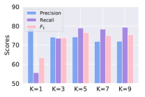
The Effect of $K$ .

As discussed in Section 2.1 and 2.2, the parameter $K$ can affect the learning procedure from two aspects. We compare the performance of different $K$ on Taobao dataset with Random-based Scheme and $\rho=0.2$ . The hyperparameter over [top $K$ ] is selected from $\{1,3,5,7,9\}$ on the validation set. As illustrated in Figure 2, a relatively large $K$ delivers better empirical results, and the metrics (precision, recall and $F_{1}$ ) are pretty close when $K=5,7,9$ . Meanwhile, a smaller $K$ can narrow down the possible paths more effectively in theory. Hence we favor $K=5$ which might be a balanced choice.

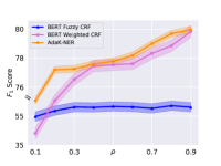
The Effect of $\rho$ .

We further examine annotation rate ( $\rho$ ) interacts with learning. We plot $F_{1}$ score on Taobao dataset with Random-based Scheme across varying annotation rate in Figure 2. The annotation removed with large $\rho$ inherits the annotation removed with the small $\rho$ . All the performance deliver better results with the increase of $\rho$ . Our model consistently outperforms weighted CRF and Fuzzy CRF, and the improvement is significant when $\rho$ is relatively small, which indicates our model is especially powerful when the annotated tokens are fairly sparse.

3.4 Ablation Study

To investigate the effectiveness of the proposed strategies used in AdaK-NER, we conduct the following ablation with Random-based Scheme and $\rho=0.2$ . As shown in Table 4, the adaptive $K$ -best loss contributes most to our model on the three datasets. It helps our model achieve higher recall while preserving acceptable precision. Especially on Youku dataset, removing it would cause a significant drop on recall by $40\%$ . The weighted CRF loss is indispensable, and annealing method could help our model achieve better results. Candidate mask is attributed to promote precision while keeping high recall. Both $K$ -best candidates and self-built candidates facilitate the model performance. Iterative sample selection makes a positive contribution to our model on CoNLL-2003 and Taobao, whereas it slightly hurts the performance on Youku. In general, incorporating these techniques enhances model performance on incomplete annotated data.

4 Related Works

Pre-trained Language Models

has been an emerging direction in NLP since Google launched BERT Devlin et al. (2018) in 2018. With the powerful Transformer architecture, several pre-trained models, such as BERT and generative pre-training model (GPT), and their variants have achieved state-of-the-art performance in various NLP tasks including NER Devlin et al. (2018); Liu et al. (2019). Yang Yang et al. (2019) proposed a pre-trained permutation language model (XLNet) to overcome the limitations of denoising autoencoding based pre-training. Liu Liu et al. (2019) demonstrated that more data and more parameter tuning could benefit pre-trained language models, and released a new pre-trained model (RoBERTa). To follow the trend, we use BERT as our neural model in this work.

Statistical Modeling

has been widely employed in sequence labeling. Classical models learn label sequences through graph-based representation, with prominent examples such as Hidden Markov Model (HMM), Maximum Entropy Markov Models (MEMM) and Conditional Random Fields (CRF) Lafferty et al. (2001). Among them, CRF is an optimal model, since it resolves the labeling bias issue in MEMM and doesn’t require the unreasonable independence assumptions in HMM. However, conventional CRF is not directly applicable to the incomplete annotation situation. Ni Ni et al. (2017) select the sentences with the highest confidence, and regarding missing labels as O. Another line of work is to replace CRF with Partial CRF Nooralahzadeh et al. (2019); Huang et al. (2019) or Fuzzy CRF Shang et al. (2018), which assign unlabeled words with all possible labels and maximize the total probability Yang et al. (2018). Although these works have led to many promising results, they still need external knowledge for high-quality performance. Jie Jie et al. (2019) presented a weighted CRF model which is most closely related to our work. They estimated a proper distribution for all possible paths derived from the incomplete annotations. Our work enhances Fuzzy CRF by reducing the possible paths by a large margin, aiming to better focus on the gold path.

5 Conclusion

In this paper, we explore how to build an effective NER model by only using incomplete annotations. We propose two major strategies including introducing a novel adaptive $K$ -best loss and a mask based on $K$ -best candidates and self-built candidates to help our model better focus on the gold path. The results show that our approaches can significantly improve the performance of NER model with incomplete annotations.

References

Cao et al. [2019] Yu Cao, Meng Fang, and Dacheng Tao. Bag: Bi-directional attention entity graph convolutional network for multi-hop reasoning question answering. arXiv preprint arXiv:1904.04969, 2019.
Cui et al. [2019] Yiming Cui, Wanxiang Che, Ting Liu, Bing Qin, Shijin Wang, and Guoping Hu. Cross-lingual machine reading comprehension. arXiv preprint arXiv:1909.00361, 2019.
Devlin et al. [2018] Jacob Devlin, Ming-Wei Chang, Kenton Lee, and Kristina Toutanova. Bert: Pre-training of deep bidirectional transformers for language understanding. arXiv preprint arXiv:1810.04805, 2018.
Effland and Collins [2021] Thomas Effland and Michael Collins. Partially supervised named entity recognition via the expected entity ratio loss. arXiv preprint arXiv:2108.07216, 2021.
Hinton et al. [2015] Geoffrey Hinton, Oriol Vinyals, and Jeff Dean. Distilling the knowledge in a neural network. arXiv preprint arXiv:1503.02531, 2015.
Huang and Chiang [2005] Liang Huang and David Chiang. Better k-best parsing. In Proceedings of the Ninth International Workshop on Parsing Technology, 2005.
Huang et al. [2019] Xiao Huang, Li Dong, Elizabeth Boschee, and Nanyun Peng. Learning a unified named entity tagger from multiple partially annotated corpora for efficient adaptation. arXiv preprint arXiv:1909.11535, 2019.
Jia et al. [2020] Chen Jia, Yuefeng Shi, Qinrong Yang, and Yue Zhang. Entity enhanced bert pre-training for chinese ner. In Proceedings of the 2020 Conference on Empirical Methods in Natural Language Processing (EMNLP), pages 6384–6396, 2020.
Jie et al. [2019] Zhanming Jie, Pengjun Xie, Wei Lu, Ruixue Ding, and Linlin Li. Better modeling of incomplete annotations for named entity recognition. In Proceedings of the 2019 Conference of the North American Chapter of the Association for Computational Linguistics: Human Language Technologies, Volume 1 (Long and Short Papers), pages 729–734, 2019.
Lafferty et al. [2001] John Lafferty, Andrew McCallum, and Fernando CN Pereira. Conditional random fields: Probabilistic models for segmenting and labeling sequence data. 2001.
Li et al. [2020] Xiaonan Li, Hang Yan, Xipeng Qiu, and Xuanjing Huang. Flat: Chinese ner using flat-lattice transformer. arXiv preprint arXiv:2004.11795, 2020.
Li et al. [2021] Yangming Li, lemao liu, and Shuming Shi. Empirical analysis of unlabeled entity problem in named entity recognition. In International Conference on Learning Representations, 2021.
Liu et al. [2019] Yinhan Liu, Myle Ott, Naman Goyal, Jingfei Du, Mandar Joshi, Danqi Chen, Omer Levy, Mike Lewis, Luke Zettlemoyer, and Veselin Stoyanov. Roberta: A robustly optimized bert pretraining approach. arXiv preprint arXiv:1907.11692, 2019.
Mayhew et al. [2019] Stephen Mayhew, Snigdha Chaturvedi, Chen-Tse Tsai, and Dan Roth. Named entity recognition with partially annotated training data. arXiv preprint arXiv:1909.09270, 2019.
Ni et al. [2017] Jian Ni, Georgiana Dinu, and Radu Florian. Weakly supervised cross-lingual named entity recognition via effective annotation and representation projection. arXiv preprint arXiv:1707.02483, 2017.
Nooralahzadeh et al. [2019] Farhad Nooralahzadeh, Jan Tore Lønning, and Lilja Øvrelid. Reinforcement-based denoising of distantly supervised ner with partial annotation. Association for Computational Linguistics, 2019.
Peng et al. [2019] Minlong Peng, Xiaoyu Xing, Qi Zhang, Jinlan Fu, and Xuanjing Huang. Distantly supervised named entity recognition using positive-unlabeled learning. arXiv preprint arXiv:1906.01378, 2019.
Poria et al. [2016] Soujanya Poria, Erik Cambria, and Alexander Gelbukh. Aspect extraction for opinion mining with a deep convolutional neural network. Knowledge-Based Systems, 108:42–49, 2016.
Sang and De Meulder [2003] Erik F Sang and Fien De Meulder. Introduction to the conll-2003 shared task: Language-independent named entity recognition. arXiv preprint cs/0306050, 2003.
Shang et al. [2018] Jingbo Shang, Liyuan Liu, Xiang Ren, Xiaotao Gu, Teng Ren, and Jiawei Han. Learning named entity tagger using domain-specific dictionary. arXiv preprint arXiv:1809.03599, 2018.
Surdeanu et al. [2010] Mihai Surdeanu, Ramesh Nallapati, and Christopher Manning. Legal claim identification: Information extraction with hierarchically labeled data. In Workshop Programme, page 22, 2010.
Wang et al. [2019] Zihan Wang, Jingbo Shang, Liyuan Liu, Lihao Lu, Jiacheng Liu, and Jiawei Han. Crossweigh: Training named entity tagger from imperfect annotations. arXiv preprint arXiv:1909.01441, 2019.
Wei et al. [2020] Qiang Wei, Zongcheng Ji, Zhiheng Li, Jingcheng Du, Jingqi Wang, Jun Xu, Yang Xiang, Firat Tiryaki, Stephen Wu, Yaoyun Zhang, et al. A study of deep learning approaches for medication and adverse drug event extraction from clinical text. Journal of the American Medical Informatics Association, 27(1):13–21, 2020.
Yang et al. [2018] Yaosheng Yang, Wenliang Chen, Zhenghua Li, Zhengqiu He, and Min Zhang. Distantly supervised ner with partial annotation learning and reinforcement learning. In Proceedings of the 27th International Conference on Computational Linguistics, pages 2159–2169, 2018.
Yang et al. [2019] Zhilin Yang, Zihang Dai, Yiming Yang, Jaime Carbonell, Russ R Salakhutdinov, and Quoc V Le. Xlnet: Generalized autoregressive pretraining for language understanding. In Advances in neural information processing systems, pages 5753–5763, 2019.

AdaK-NER: An Adaptive Top-𝐊\mathbf{K} Approach for Named Entity Recognition with Incomplete Annotations

Abstract

1 Introduction

2 Proposed Approach

2.1 Adaptive KK-best Loss

2.2 Estimating qq with Candidate Mask

KK-best Candidates.

Self-built Candidates.

2.3 Annealing Technique for λ\lambda

2.4 Iterative Sample Selection

3 Experiments

3.1 Dataset

3.2 Experiment Setup

Evaluation Metrics.

Baselines.

Training details.

3.3 Experimental Results

The Effect of KK.

The Effect of ρ\rho.

3.4 Ablation Study

4 Related Works

Pre-trained Language Models

Statistical Modeling

5 Conclusion

References

AdaK-NER: An Adaptive Top- $\mathbf{K}$ Approach
for Named Entity Recognition with Incomplete Annotations

2.1 Adaptive $K$ -best Loss

2.2 Estimating $q$ with Candidate Mask

$K$ -best Candidates.

2.3 Annealing Technique for $\lambda$

The Effect of $K$ .

The Effect of $\rho$ .