Adaptation for Validation of a Consolidated Control Barrier Function based Control Synthesis

Since the arrival of control barrier functions (CBFs) to the field of safety-critical systems [1], much attention has been devoted to the development of their viability for safe control design [2, 3, 4]. As a set-theoretic approach founded on the notion of forward invariance, CBFs encode safety in that they ensure that any state beginning in a safe set remains so for all future time. In the context of control design, CBF conditions are often used as constraints in quadratic program (QP) based control laws, either as safety filters [5] or in conjunction with stability constraints (e.g. control Lyapunov functions) [6]. Their utility has been successfully demonstrated for a variety of safety-critical applications, including mobile robots [7, 8], unmanned aerial vehicles (UAVs) [9, 10], and autonomous driving [11, 12]. But while it is now well-established that CBFs for controlled dynamical systems serve as certificates of safety, the verification of candidate CBFs as valid is in general a challenging problem.

Though for a single CBF there exist guarantees of validity under certain conditions for systems with either unbounded [2] or bounded control authority [13, 14], these results do not generally extend to control systems seeking to satisfy multiple candidate CBF constraints. Recent approaches to control design in the presence of multiple CBF constraints have mainly circumvented this challenge by considering only one such constraint at a given time instance, either by assumption [15] or construction in a non-smooth manner [16, 17]. In contrast, the authors of [18] and [19] each propose smoothly synthesizing one candidate CBF for the joint satisfaction of multiple constraints, but make no attempt to validate their candidate function. The problem of safe control design under a multitude of constraints is especially relevant in practical applications involving autonomous mobile robots, where the main challenge is in the robot completing its nominal objective while satisfying constraints related to collision avoidance with respect to obstacles both static and dynamic.

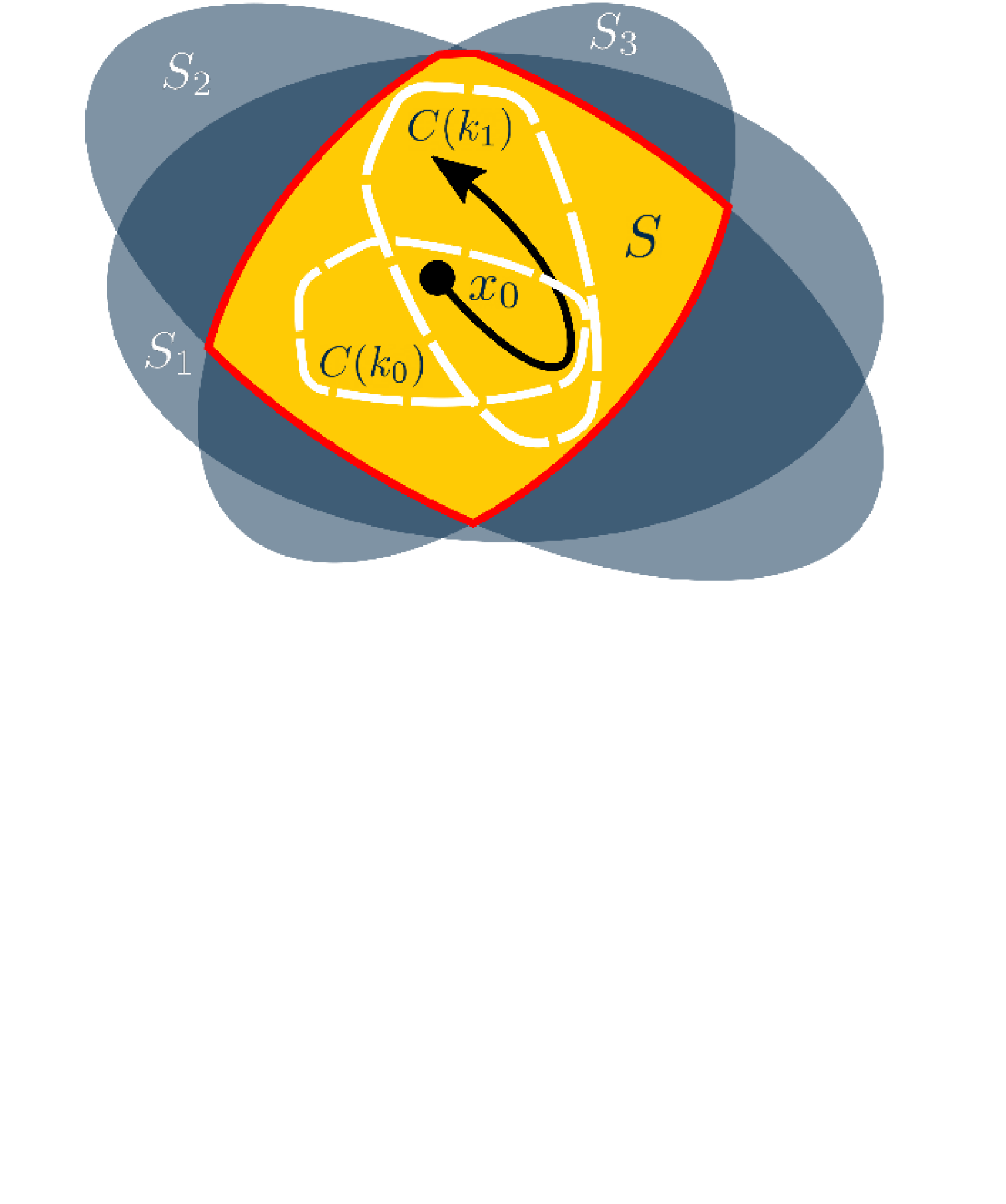
It is with this problem in mind that we propose a consolidated CBF (C-CBF) based approach to control design for multi-agent systems in the presence of both non-communicative and non-responsive (though non-adversarial) agents. Constructed by smoothly synthesizing any arbitrary number of candidate CBFs into one, our C-CBF defines a new super-level set that can under-approximate the intersection of its constituent sets arbitrarily closely (see Figure 1). We further propose a parameter adaptation law for the weighting of the constituent functions, and prove that its use renders our C-CBF valid and the super-level set controlled invariant for the class of nonlinear, control-affine, multi-agent systems under consideration. And while various works have utilized parameter adaptation in the context of control for safety-critical systems, usually in an attempt to either learn [20, 21] or compensate for [22] unknown parameters in the system dynamics, our proposed adaptation law is the first to our knowledge to be used for the simultaneous verified satisfaction of multiple CBF constraints. To show the effectiveness of our proposed control formulation, we study a decentralized multi-robot goal-reaching problem in a crowded warehouse environment amongst non-responsive agents. As a practical demonstration, we tested our controller experimentally on a collection of ground rovers in the laboratory setting and found that it succeeded in safely driving the rovers to their goal locations amongst non-responsive agents behaving both aggressively and conservatively.

The paper is organized as follows. Section II introduces some preliminaries, including set invariance, optimization based control, and our first problem statement. In Section III, we introduce the form of our C-CBF and propose a parameter adaptation law for rendering it valid. Sections IV and V contain the results of our simulated and experimental case studies respectively, and in Section VI we conclude with final remarks and directions for future work.

We use the following notation throughout the paper. $\mathbb{R}$ denotes the set of real numbers. The set of integers between $i$ and $j$ (inclusive) is $[i..j]$. $\|\cdot\|$ represents the Euclidean norm. A function $\alpha:\operatorname{\mathbb{R}}\rightarrow\operatorname{\mathbb{R}}$ is said to belong to class $\mathcal{K}_{\infty}$ if $\alpha(0)=0$ and $\alpha$ is increasing on the interval $(-\infty,\infty)$, A function $\phi:\operatorname{\mathbb{R}}\times\operatorname{\mathbb{R}}\rightarrow\operatorname{\mathbb{R}}$ is said to belong to class $\mathcal{L}\mathcal{L}$ if for each fixed $r$ (resp. $s$), the function $\phi(r,s)$ is decreasing with respect to $s$ (resp. $r$) and is such that $\phi(r,s)\rightarrow 0$ for $s\rightarrow\infty$ (resp. $r\rightarrow\infty$). The Lie derivative of a function $V:\mathbb{R}^{n}\rightarrow\mathbb{R}$ along a vector field $f:\mathbb{R}^{n}\rightarrow\mathbb{R}^{n}$ at a point $x\in\mathbb{R}^{n}$ is denoted $L_{f}V(x)\triangleq\frac{\partial V}{\partial x}f(x)$.

In this paper we consider a multi-agent system, each of whose $A$ constituent agents may be modelled by the following class of nonlinear, control-affine dynamical systems:

where $\bm{x}_{i}\in\operatorname{\mathbb{R}}^{n}$ and $\bm{u}_{i}\in\mathcal{U}_{i}\subseteq\operatorname{\mathbb{R}}^{m}$ are the state and control input vectors for the i^th agent, with $\mathcal{U}_{i}$ the input constraint set, and where $f_{i}:\operatorname{\mathbb{R}}^{n}\rightarrow\operatorname{\mathbb{R}}^{n}$ and $g_{i}:\operatorname{\mathbb{R}}^{n\times m}\rightarrow\operatorname{\mathbb{R}}^{n}$ are known, locally Lipschitz, and not necessarily homogeneous $\forall i\in\mathcal{A}=[1..A]$. We denote the concatenated state vector as $\bm{x}=[\bm{x}_{1},\ldots,\bm{x}_{A}]^{T}\in\operatorname{\mathbb{R}}^{N}$, the concatenated control input vector as $\bm{u}=[\bm{u}_{1},\ldots,\bm{u}_{A}]^{T}\in\mathcal{U}\subseteq\operatorname{\mathbb{R}}^{M}$, and as such express the full system dynamics as

where $F=[f_{1},\ldots,f_{A}]^{T}:\operatorname{\mathbb{R}}^{N}\rightarrow\operatorname{\mathbb{R}}^{N}$ and $G=\textrm{diag}([g_{1},\ldots,g_{A}]):\operatorname{\mathbb{R}}^{M\times N}\rightarrow\operatorname{\mathbb{R}}^{N}$. We assume that a (possibly empty) subset of the agents are communicative, denoted $j\in\mathcal{A}_{c}=[1..A_{c}]$, in the sense that they share information (e.g. states, control objectives, etc.) with one another, and that the remaining agents are non-communicative, denoted $k\in\mathcal{A}_{n}=[(A_{c}+1)..A]$, in that they do not share information, where $A_{c}\geq 0$ and $A_{n}=A-A_{c}\geq 0$ are the number of communicative and non-communicative agents respectively. We further assume that all agents are non-adversarial in that they do not seek to damage or otherwise deceive others, though there may be non-communicative agents which are non-responsive ($l\in\mathcal{A}_{n,n}\subseteq\mathcal{A}_{n}$) in that they do not actively avoid unsafe situations.

In this section, we first introduce our proposed solution to Problem 1, a consolidated control barrier function (C-CBF) candidate that smoothly synthesizes multiple candidate CBFs into one, and then design a parameter adaptation law which renders the candidate C-CBF valid for safe control design.

In this section, we demonstrate our C-CBF controller on a decentralized multi-robot goal-reaching problem.

Consider a collection of 3 non-communicative, but responsive robots ($i\in\mathcal{A}_{n}\setminus\mathcal{A}_{n,n}$) in a warehouse environment seeking to traverse a narrow corridor intersected by a passageway occupied with 6 non-responsive agents ($j\in\mathcal{A}_{n,n}$). The non-responsive agents may be e.g. humans walking or some other dynamic obstacles. Let $\mathcal{F}$ be an inertial frame with a point $s_{0}$ denoting its origin, and assume that each robot may be modeled according to a dynamic extension of the kinematic bicycle model described by [31, Ch. 2], provided here for completeness:

where $x_{i}$ and $y_{i}$ denote the position (in m) of the center of gravity (c.g.) of the i^th robot with respect to $s_{0}$, $\psi_{i}$ is the orientation (in rad) of its body-fixed frame, $\mathcal{B}_{i}$, with respect to $\mathcal{F}$, $\beta_{i}$ is the slip angle¹¹1$\beta_{i}$ is related to the steering angle $\delta_{i}$ via $\tan{\beta_{i}}=\frac{l_{r}}{l_{r}+l_{f}}\tan{\delta_{i}}$, where $l_{f}+l_{r}$ is the wheelbase with $l_{f}$ (resp. $l_{r}$) the distance from the c.g. to the center of the front (resp. rear) wheel. (in rad) of the c.g. of the vehicle relative to $\mathcal{B}_{i}$ (assume $|\beta_{i}|<\frac{\pi}{2}$), and $v_{i}$ is the velocity of the rear wheel with respect to $\mathcal{F}$. The state of robot $i$ is denoted $\bm{z}_{i}=[x_{i}\;y_{i}\;\psi_{i}\;\beta_{i}\;v_{i}]^{T}$, and its control input is $\bm{u}_{i}=[a_{i}\;\omega_{i}]^{T}$, where $a_{i}$ is the acceleration of the rear wheel (in m/s²), and $\omega_{i}$ is the angular velocity (in rad/s) of $\beta_{i}$.

The challenges of this scenario relate to preserving safety despite multiple non-communicative and non-responsive agents present in a constrained environment. A robot is safe if it 1) obeys the speed restriction, 2) remains inside the corridor area, and 3) avoids collisions with all other robots. Speed is addressed with the following candidate CBF:

where $s_{M}>0$, while for corridor safety and collision avoidance we used forms of the relaxed future-focused CBF introduced in [11] for roadway intersections, namely

where (23) prevents collisions with the corridor walls (defined as lines in the $xy$-plane via $m_{L},b_{L},m_{R},b_{R}\in\operatorname{\mathbb{R}}$), and (24) prevents inter-robot collisions and is defined $\forall i\in\mathcal{A}_{n}\setminus\mathcal{A}_{n,n}$, $\forall j\in\mathcal{A}_{n}$, where $\epsilon>0$, $D(\bm{z}_{i},\bm{z}_{j},t_{a})$ is the Euclidean distance between agents $i$ and $j$ at arbitrary time $t_{a}$, and $\hat{\tau}$ denotes the time in the interval $[0,T]$ at which the minimum inter-agent distance will occur under constant velocity future trajectories. For a more detailed discussion on future-focused CBFs, see [11]. As such, (22), (23), and (24) define the sets

the intersection of which constitutes the safe set for agents $i$, i.e. $S_{i}(t)=S_{v,i}\cap S_{c,i}\cap S_{r,i}$.

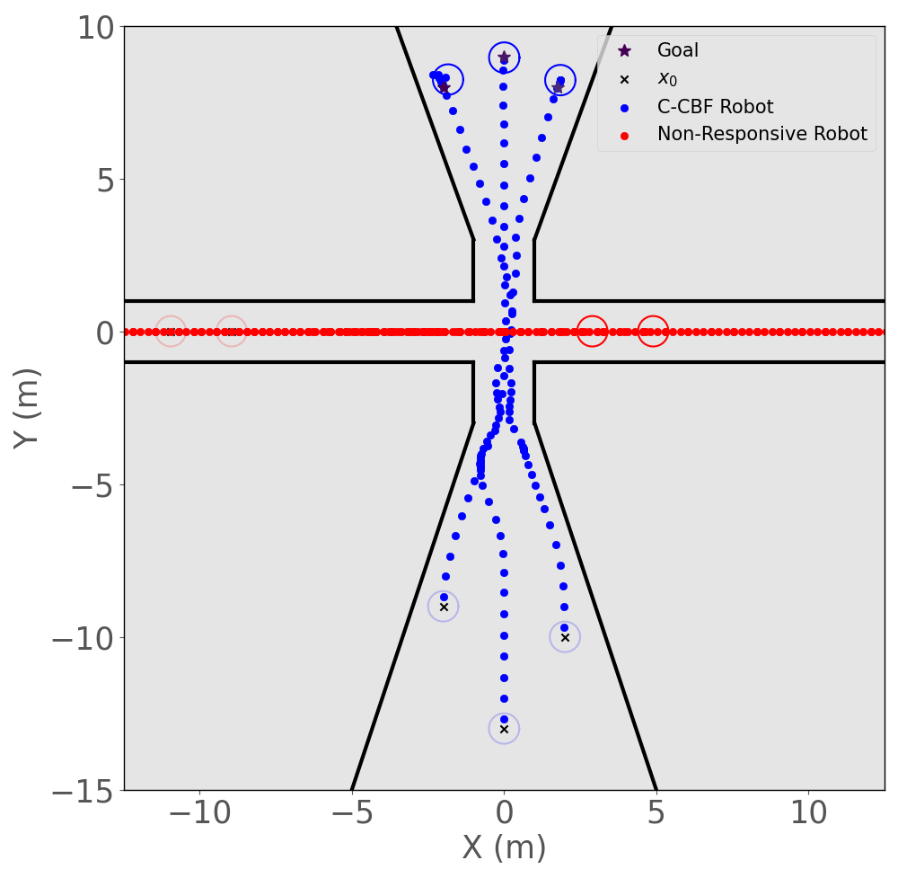
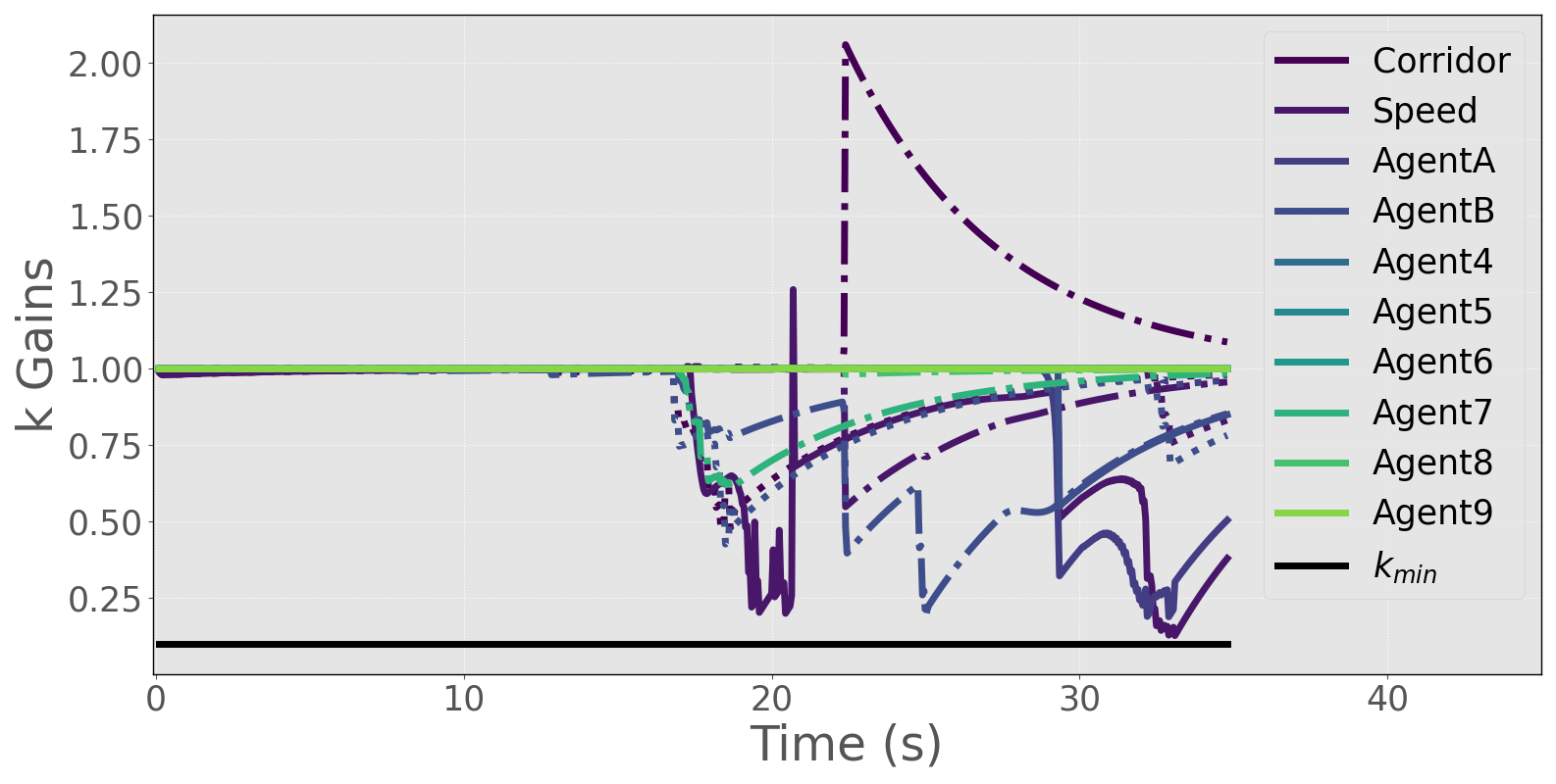
We control robots $i\in\mathcal{A}_{n}\setminus\mathcal{A}_{n,n}$ using a C-CBF based decentralized controller of the form (20) with constituent functions $h_{c}$, $h_{s}$, $h_{r}$, an LQR based nominal control input (see [11, Appendix 1]), and initial gains $\bm{k}(0)=\mathbf{1}_{10\times 1}$. The non-responsive agents used a similar LQR controller to move through the passageway in pairs of two, with the first two pairs passing through the intersection without stopping and the last pair stopping at the intersection before proceeding.

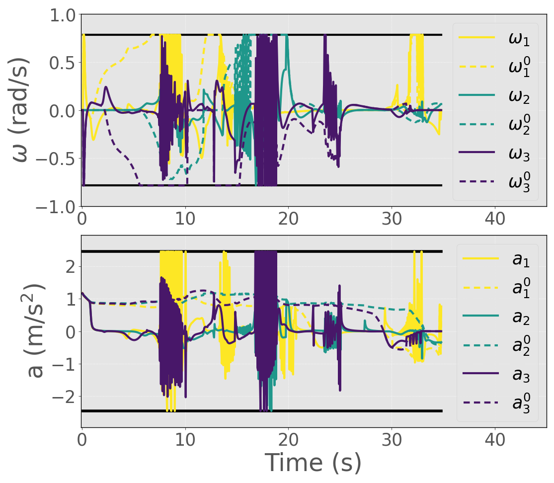
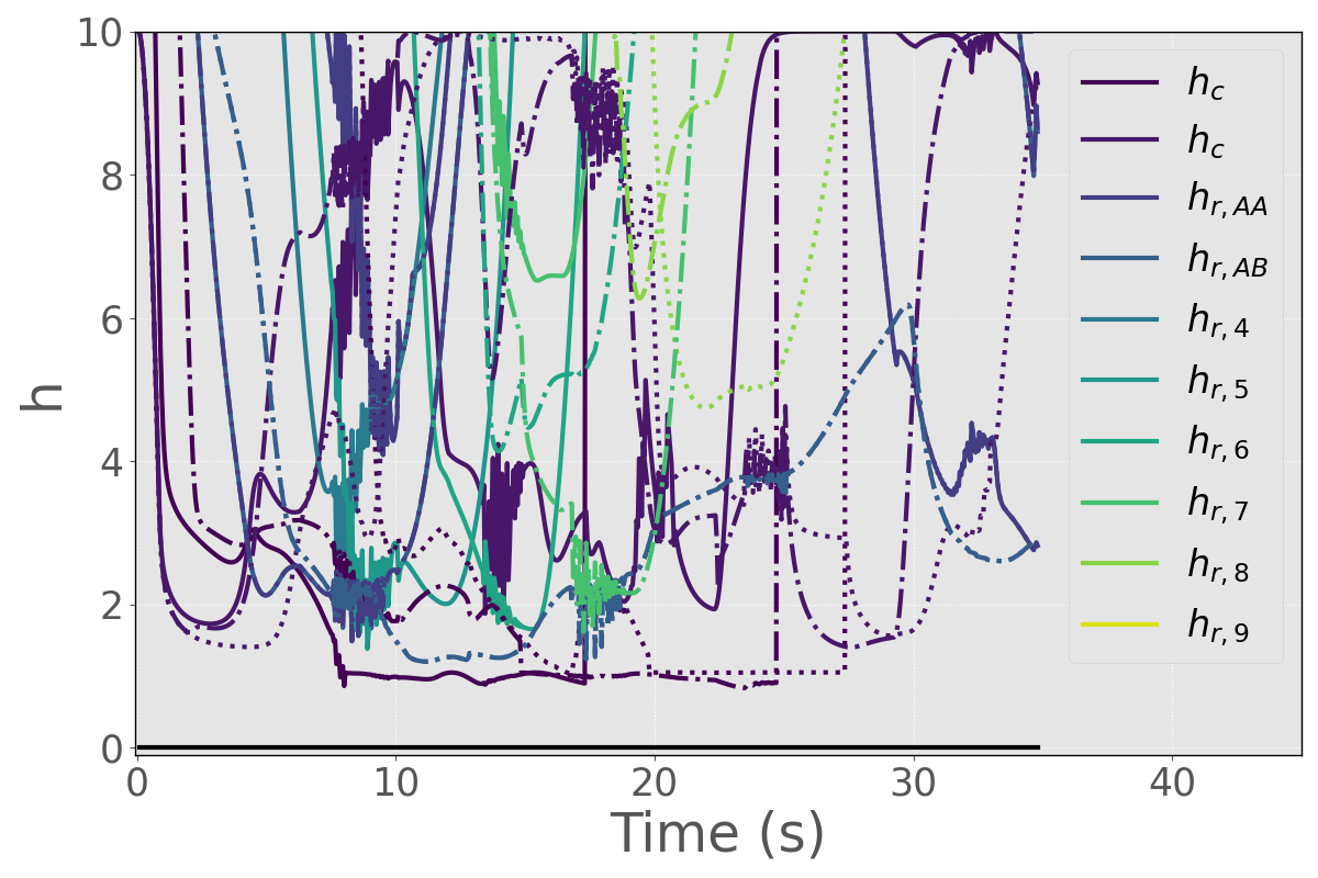
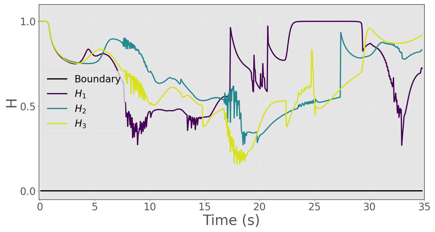
As shown in Figure 2, the non-communicative robots traverse both the narrow corridor and the busy intersection to reach their goal locations safely. The trajectories of the gains $\bm{k}$ for each warehouse robot are shown in Figure 3, while their control inputs are depicted in Figure 4. The CBF time histories for the constituent and consolidated functions are highlighted in Figures 5 and 6 respectively, and show that the C-CBF controllers maintained safety at all times.

For experimental validation of our approach, we used an AION R1 UGV ground rover as an ego vehicle in the laboratory setting and required it to reach a goal location in the presence of two non-responsive rovers: one static and one dynamic. We modeled the rovers as bicycles using (21), and sent angular rate $\omega_{i}$ and velocity $v_{i}$ (numerically integrated based on the controller’s acceleration output) commands to the rovers’ on-board PID controllers. The ego rover used our proposed C-CBF (20) with constituent candidate CBFs (22) (with $s_{M}=1$ m/s) and the rff-CBF defined in (24) for collision avoidance. The nominal input to the C-CBF controller was the LQR law from the warehouse robot example, as was the controller used by the dynamic non-responsive rover. A Vicon motion capture system was used for position feedback, and the state estimation was performed by extended Kalman filter via the on-board PX4.

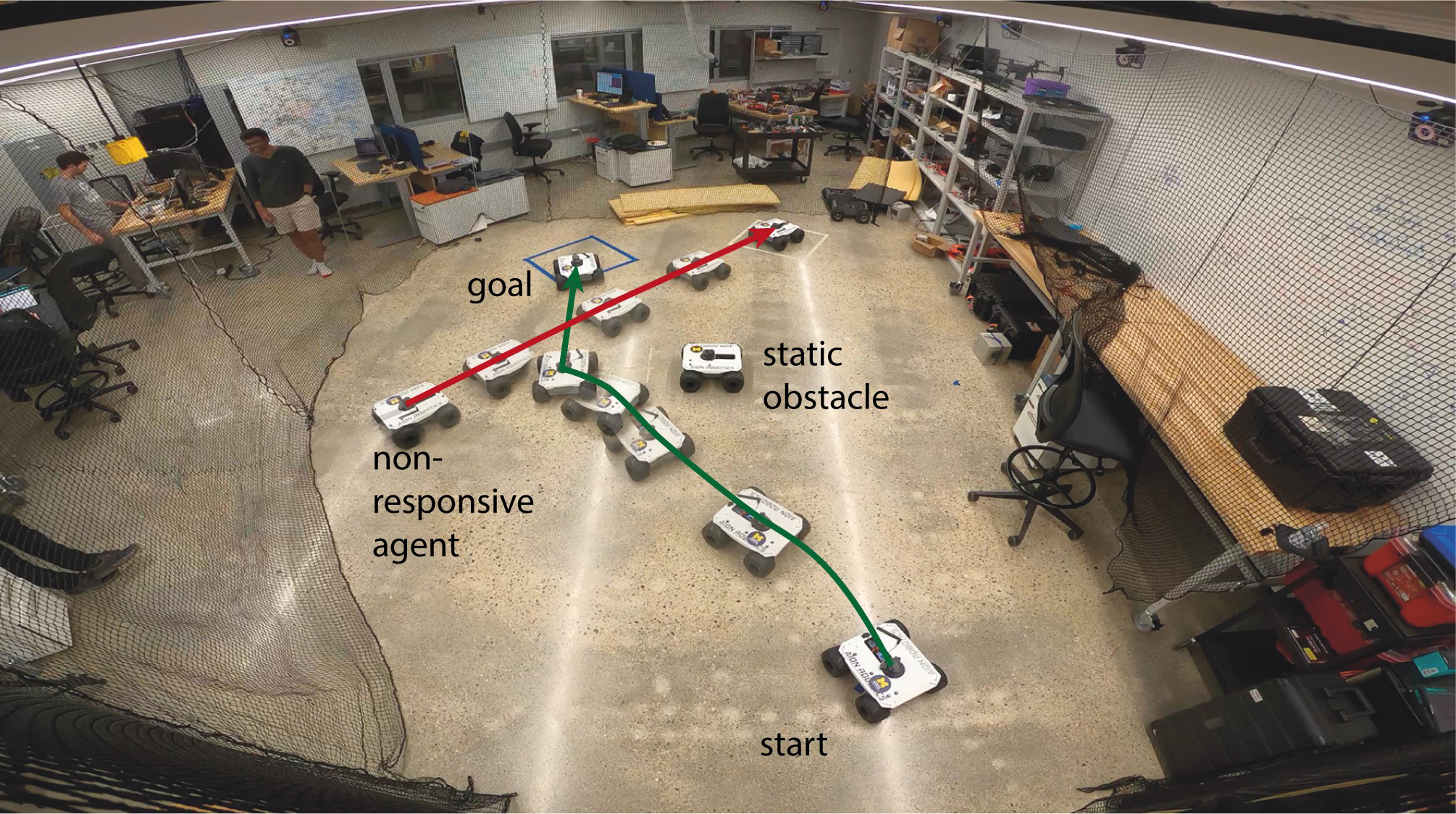
For the setup, the static rover was placed directly between the ego rover and its goal, while the dynamic rover was stationary until suddenly moving across the ego’s path as it approached its target. As highlighted in Figure 7, the ego rover first headed away from the static rover and then decelerated and swerved to avoid a collision with the second rover before correcting course and reaching its goal. Videos and code for both this experiment and the simulation in Section IV is available on Github²²2Link to Github repo: github.com/6lackmitchell/CCBF-Control.

In this paper, we addressed the problem of safe control under multiple state constraints via a C-CBF based control design. To ensure that the synthesized C-CBF is valid, we introduced a parameter adaptation law on the weights of the C-CBF constituent functions and proved that the resulting controller is safe. We then demonstrated the success of our approach on a multi-robot control problem in a crowded warehouse environment, and further validated our work on a ground rover experiment in the lab.

In the future, we plan to explore conditions under which the C-CBF approach may preserve guarantees in the presence of input constraints, including whether alternative adaptation laws for the weights assist in guarantees of liveness in addition to safety.

References

- [1] P. Wieland and F. Allgöwer, “Constructive safety using control barrier functions,” IFAC Proceedings Vols., vol. 40, no. 12, pp. 462–467, 2007.
- [2] A. D. Ames, X. Xu, J. W. Grizzle, and P. Tabuada, “Control barrier function based quadratic programs for safety critical systems,” IEEE Trans. on Automatic Control, vol. 62, no. 8, pp. 3861–3876, 2017.
- [3] W. Xiao and C. Belta, “Control barrier functions for systems with high relative degree,” in IEEE 58th Conference on Decision and Control (CDC), 2019, pp. 474–479.
- [4] W. S. Cortez, D. Oetomo, C. Manzie, and P. Choong, “Control barrier functions for mechanical systems: Theory and application to robotic grasping,” in IEEE Trans. on Control Systems Tech., 2019, pp. 1–16.
- [5] Y. Chen, H. Peng, and J. Grizzle, “Obstacle avoidance for low-speed autonomous vehicles with barrier function,” IEEE Transactions on Control Systems Technology, vol. 26, no. 1, pp. 194–206, 2018.
- [6] K. Garg and D. Panagou, “Robust control barrier and control lyapunov functions with fixed-time convergence guarantees,” in 2021 American Control Conference (ACC), 2021, pp. 2292–2297.
- [7] Y. Chen, A. Singletary, and A. D. Ames, “Guaranteed obstacle avoidance for multi-robot operations with limited actuation: A control barrier function approach,” IEEE Control Systems Letters, vol. 5, no. 1, pp. 127–132, 2021.
- [8] M. Jankovic and M. Santillo, “Collision avoidance and liveness of multi-agent systems with cbf-based controllers,” in 2021 60th IEEE Conference on Decision and Control (CDC), 2021, pp. 6822–6828.
- [9] B. Xu and K. Sreenath, “Safe teleoperation of dynamic uavs through control barrier functions,” in 2018 IEEE International Conference on Robotics and Automation (ICRA), 2018, pp. 7848–7855.
- [10] M. Khan, M. Zafar, and A. Chatterjee, “Barrier functions in cascaded controller: Safe quadrotor control,” in 2020 American Control Conference (ACC), 2020, pp. 1737–1742.
- [11] M. Black, M. Jankovic, A. Sharma, and D. Panagou, “Intersection crossing with future-focused control barrier functions,” arXiv preprint arXiv:2204.00127, 2022.
- [12] S. Yaghoubi, G. Fainekos, T. Yamaguchi, D. Prokhorov, and B. Hoxha, “Risk-bounded control with kalman filtering and stochastic barrier functions,” in 2021 60th IEEE Conference on Decision and Control (CDC), 2021, pp. 5213–5219.
- [13] J. Breeden and D. Panagou, “High relative degree control barrier functions under input constraints,” in 2021 60th IEEE Conference on Decision and Control (CDC), 2021, pp. 6119–6124.
- [14] W. Xiao, C. Belta, and C. G. Cassandras, “Adaptive control barrier functions,” IEEE Transactions on Automatic Control, vol. 67, no. 5, pp. 2267–2281, 2022.
- [15] W. S. Cortez, X. Tan, and D. V. Dimarogonas, “A robust, multiple control barrier function framework for input constrained systems,” IEEE Control Systems Letters, vol. 6, pp. 1742–1747, 2022.
- [16] P. Glotfelter, J. Cortes, and M. Egerstedt, “Nonsmooth barrier functions with applications to multi-robot systems,” IEEE Control Systems Letters, vol. 1, pp. 310–315, 10 2017.
- [17] Y. Huang and Y. Chen, “Switched Control Barrier Function With Applications to Vehicle Safety Control,” ser. Dynamic Systems and Control Conference, vol. 1, 10 2020.
- [18] L. Lindemann and D. V. Dimarogonas, “Control barrier functions for signal temporal logic tasks,” IEEE Control Systems Letters, vol. 3, no. 1, pp. 96–101, 2019.
- [19] M. Machida and M. Ichien, “Consensus-based control barrier function for swarm,” in 2021 IEEE International Conference on Robotics and Automation (ICRA), 2021, pp. 8623–8628.
- [20] M. Black, E. Arabi, and D. Panagou, “Fixed-time parameter adaptation for safe control synthesis,” arXiv preprint arXiv:2204.10453, 2022.
- [21] B. T. Lopez, J.-J. E. Slotine, and J. P. How, “Robust adaptive control barrier functions: An adaptive and data-driven approach to safety,” IEEE Control Systems Letters, vol. 5, no. 3, pp. 1031–1036, 2021.
- [22] A. J. Taylor and A. D. Ames, “Adaptive safety with control barrier functions,” in 2020 American Control Conference (ACC), 2020, pp. 1399–1405.
- [23] T. Gurriet, A. Singletary, J. Reher, L. Ciarletta, E. Feron, and A. Ames, “Towards a framework for realizable safety critical control through active set invariance,” in 9th ACM/IEEE International Conference on Cyber-Physical Systems (ICCPS), 2018, pp. 98–106.
- [24] S. Kolathaya and A. D. Ames, “Input-to-state safety with control barrier functions,” IEEE Control Systems Letters, vol. 3, no. 1, pp. 108–113, 2019.
- [25] F. Blanchini, “Set invariance in control,” Automatica, vol. 35, no. 11, pp. 1747–1767, 1999.
- [26] M. Jankovic, M. Santillo, and Y. Wang, “Multi-agent systems with cbf-based controllers – collision avoidance and liveness from instability,” arXiv preprint arXiv:2207.04915, 2022.
- [27] U. Borrmann, L. Wang, A. D. Ames, and M. Egerstedt, “Control barrier certificates for safe swarm behavior,” IFAC-PapersOnLine, vol. 48, no. 27, pp. 68–73, 2015.
- [28] L. Wang, A. D. Ames, and M. Egerstedt, “Safety barrier certificates for collisions-free multirobot systems,” vol. 33, no. 3. IEEE, 2017, pp. 661–674.
- [29] H. Parwana and D. Panagou, “Trust-based rate-tunable control barrier functions for non-cooperative multi-agent systems,” arXiv preprint arXiv:2204.04555, 2022.
- [30] T. F. Coleman and D. C. Sorensen, “A note on the computation of an orthonormal basis for the null space of a matrix,” Mathematical Programming, vol. 29, pp. 234–242, 6 1984.
- [31] R. Rajamani, Vehicle Dynamics and Control. Springer US, 2012.