Adaptive Anchored Inversion for Gaussian
Random Fields
Using Nonlinear Data
Abstract
In a broad and fundamental type of “inverse problems” in science, one infers a spatially distributed physical attribute based on observations of processes that are controlled by the spatial attribute in question. The data-generating field processes, known as “forward processes”, are usually nonlinear with respect to the spatial attribute, and are often defined non-analytically by a numerical model. The data often contain a large number of elements with significant inter-correlation. We propose a general statistical method to tackle this problem. The method is centered on a parameterization device called “anchors” and an iterative algorithm for deriving the distribution of anchors conditional on the observed data. The algorithm draws upon techniques of importance sampling and multivariate kernel density estimation with weighted samples. Anchors are selected automatically; the selection evolves in iterations in a way that is tailored to important features of the attribute field. The method and the algorithm are general with respect to the scientific nature and technical details of the forward processes. Conceptual and technical components render the method in contrast to standard approaches that are based on regularization or optimization. Some important features of the proposed method are demonstrated by examples from the earth sciences, including groundwater flow, rainfall-runoff, and seismic tomography.
Key words: adaptive model selection, dimension reduction, inverse problem, iterative algorithm, spatial statistics.
Department of Mathematics and Statistics, University of Alaska, Fairbanks, Alaska, USA.
Published as Inverse Problems 27(2011) 125011. doi:10.1088/0266-5611/27/12/125011
1 Introduction
Consider a spatial Gaussian process (also called a Gaussian random field) , where , being the model domain, and . Define a nonlinear functional of this field: , where is a vector of length . Suppose we have observed the value of this functional, say the vector value is . Conditional on this observation, how can we characterize the field ?
This is an abstraction of statistical approaches to a wide range of scientific questions. In these questions, is a “spatially-distributed” physical attribute. The functional , known as the “forward model” or “forward process”, is typically embodied in a deterministic, numerical algorithm that takes the field as input and outputs vector-valued result . In nature, the forward model is a physical process whose outcome is dictated by the attribute in the entire domain . The task is, conditional on the observed outcome of the forward model, how can we characterize (or “back out”) the attribute field ? Since we are using the outcome of the forward model to infer the quantity that dictates the outcome of the forward model, this task is known as an “inverse problem”.
A few examples will make the setting clear.
Example 1. Yeh [1986] reviews techniques for the groundwater inverse problem, in which the spatial attribute of interest is hydraulic conductivity of the subsurface medium. Conductivity controls groundwater flow which is governed by well-understood partial differential equations. Scientists or engineers make observations of groundwater movement to get head (i.e. pressure) and flux at selected locations and times, and attempt to use these data to infer the spatially distributed conductivity.
Example 2. Bube and Burridge [1983] study a 1-D problem in exploration seismology. In this setting, an impulsive or vibrating load applied at the ground surface launches elastic waves into the earth’s interior. Part of the wave energy is reflected by the medium and reaches the ground surface, where it is monitored at many time instants. Wave propagation in the subsurface column is described by a hyperbolic equation system with mechanic attributes of the elastic medium, including density and Lamé constants, as input parameters. The task is to recover the mechanic attributes, ideally everywhere in the subsurface column, using surface measurements of wave propagation including pressure and particle velocity.
Example 3. Newsam and Enting [1988] deduce the spatial distribution of sources (including sinks) on the surface of the globe, given time-series observations of surface concentrations of at some 20 locations around the globe. The source here is treated as a spatial attribute defined for every location on the ground surface. The surface concentration around the globe is the result of re-distribution of the sources via a transport process, governed by a diffusion equation.
These examples have three components in common: a spatial attribute of interest (hydraulic conductivity of flow media; mechanic properties of elastic media; source/sink of CO2), a forward process (groundwater flow; wave propagation; atmospheric transport), and observed outcomes of the forward process (head and flux; pressure and particle velocity; CO2 concentration). The attribute of interest varies in space and is possibly highly heterogeneous; in some scientific literature it is called a “(spatially) distributed parameter” [Kravaris and Seinfeld, 1985; Beven, 1993; Nakagiri, 1993]. The forward process is represented by a numerical model, which takes the spatial attribute as the main input, along with boundary and initial conditions. Usually, the need for this inversion arises because the attribute is needed for modeling (or simulating, or predicting) some other process of interest.
In concept, the unknown, , has infinite dimensions. In real-world applications, it is almost always defined on a finite grid that discretizes the model domain. In either case, the unknown has many more dimensions than the known . This makes the inverse problem a severely under-determined one. It has become an established strategy to formulate the inverse problem in a statistical way [Kirsch, 1996; Kaipio and Somersalo, 2005], that is, take as a random field and try to obtain its conditional distribution given the observation , i.e. . Typically, this conditional distribution is represented empirically by a large number of realizations (i.e. simulations) of the random field. In this context, Bayesian approaches and Markov chain Monte Carlo computations have been widely used (see section 2).
In this study, we propose a method for this inverse problem. The proposal centers on a parameterization device called “anchors”, hence the name of the method—“anchored inversion”. Let the anchor parameters be denoted by . With anchor parameterization, we solve a reduced problem, namely, rather than . The dimension of is much lower than that of (the latter could be infinite), and the dimension of is under the user’s control. This dimension reduction brings advantages in computation as well as conceptualization.
The proposed method is a fundamental departure from some existing approaches. In section 2, we identify some challenges faced by existing methods, which motivate the concept of “anchor”. Anchor parameterization is formally described in section 3. Section 4 presents an iterative algorithm that approximates the posterior distribution of the chosen anchor parameter () by a normal mixture. In section 5 we describe a strategy for choosing anchor parameters automatically and adaptively as the iterative algorithm proceeds. This efficient strategy makes anchor parameters evolve in iterations, adapted to the available data, complexity of the field, and the computational effort so far invested. This anchor-selection procedure is integrated into the algorithm described in section 4.
Section 6 describes two extensions to the basic framework presented in earlier sections. The first extension, geostatistical parameterization, is expected to be used in most applications. The second extension is used whenever the type of data described there are available. In section 7, the method is applied to three scientific questions using synthetic data. Section 8 concludes with a summary and highlights.
We emphasize “nonlinear” in this study, because treatment of “linear” forward models is relatively mature. A mainstay of the approaches is the Kalman filter and variants [Welch and Bishop, 1995]. However, the vast majority of forward processes in scientific applications are nonlinear, as demonstrated in section 7. Linear data, if available, are accommodated as described in section 6.2.
Although is “point-referenced” in concept, in practice the model domain is discretized (or aggregated) into a numerical grid. This discretization is assumed throughout, and it enables the use of matrix notations instead of integrals. We shall use and as generic symbols for location and the spatial variable, and use and for the finite-length and vectors corresponding to the numerical grid. Specific values of and are denoted by and , respectively. Throughout, the symbol denotes a normal density or likelihood function. We use as a generic symbol for probability density function and for conditional density. When we have a specific density, say obtained by approximation, we use a specific symbol, for example .
2 Motivation and rationale for the concept of anchor
Discretization of the model domain, along with other sources, introduces model error in the simulation of the forward process, . In addition there may be measurement error in . Suppose the model and measurement errors are additive, we can write
| (1) |
where is the forward data, is the forward model (i.e. a functional of the discretized field ), and is combined model and measurement error.
A typical Bayesian approach takes as the parameter vector and seeks its posterior distribution given the observation . Suppose the density of the error is known to be , then the likelihood function is
| (2) |
Upon specification of a prior , the posterior is . This high-dimensional posterior distribution is usually represented by samples from it via Markov chain Monte Carlo (MCMC) or related methods. There exist a large number of studies along this line, e.g. van Leeuwen and Evensen [1996]; Lee et al. [2002]; Sambridge and Mosegaard [2002]; Kaipio and Somersalo [2005]; Tarantola [2005]. If the error is multiplicative with known distribution, manipulations may be possible in simple cases; see Kaipio and Somersalo [2005, p. 58] for an example. The construct above is also the cornerstone for a large class of approaches using “regularization” and optimization [Tikhonov and Arsenin, 1977; Kravaris and Seinfeld, 1985; Engl and Neubauer, 2000; Tenorio, 2001; Doherty, 2003].
We recognize three difficulties in this approach, namely, (1) that the same is both the model parameter and the input to the forward model creates conflicting requirements; (2) the formulation is centered at “error”, , ruling out situations where error is nonexistent or negligible; (3) distribution of the error , especially the model error, is hard to specify. These points are elaborated below. Additional comments can be found in O’Sullivan [1986].
-
(1)
By taking the entire model grid as the parameter vector, the dimension of the parameter space is tied to the spatial resolution of the numerical implementation of the forward model . This creates conflicts between parameter identifiability and accuracy in the numerical forward model , which is the essential connection between the model parameter and data. One side of this paradox calls for a coarse grid (for better identification of the model parameter) whereas the other side prefers a fine grid (for more accurate simulation of the forward process).
-
(2)
The only randomness in the parameter-data link in this formulation arises from the model and measurement errors, , because the forward model is deterministic. While in reality error usually exists, in synthetic or theoretical studies it does not have to. Clearly, the Bayesian approach centered at (2) does not apply if error is nonexistent. On the other hand, even if the magnitude of the error is not quite negligible, one may elect to ignore errors (because, for example, knowledge about the error’s distribution is very limited and unreliable) and still have a meaningful inverse problem of inferring from . However, the formulation based on (1) is not applicable in this situation.
-
(3)
Reliable knowledge of the error distribution, , is often unavailable. A major complication here is model error. While one may have a decent knowledge of the measurement error based on instrument specifications, model error is much more elusive. There are numerous sources for model error, including spatial and temporal discretization, inaccurate boundary and initial conditions, relevant physics that are omitted from consideration, and so on. Another notable error stems from the so-called incommensurability [Ginn and Cushman, 1990], i.e. the fact that what is computed by the model and what is measured in the field are not exactly the same quantity. A common cause of incommensurability is discrepancy in the spatiotemporal resolution (or scale). Taken as a random vector, the model error usually has inter-correlated components. To further complicate the matter, the distribution of this error vector may depend on the input field .
Sambridge and Mosegaard [2002] point out that it is especially difficult to know the statistics of all errors when “the theoretical predictions from a model involve approximations”. However, all the sources of model error listed above essentially result in approximations.
The fact that contains model error has been emphasized by Scales and Tenorio [2001]; Lee et al. [2002]; Higdon et al. [2003]. At this point it must be recognized that model error may not be smaller than measurement error, hence it is not feasible to assume that measurement error dominates model error and makes the latter negligible. Tarantola and Valette [1982] give a telling example: “In seismology, the theoretical error made by solving the forward travel time problem is often one order of magnitude larger than the experimental error of reading the arrival time on a seismogram.” Also see Schoups et al. [2010].
We present an alternative approach that has the potential to alleviate these difficulties. The first intuition comes from the difficulty (1) above. Realizing that it is largely hopeless to aim for a sharp resolution of, say, a field using a data vector of length 100, we ask, “Instead of taking on the entire field , what about aiming for a sharper resolution of, say, 50 ‘characteristic values’ of using the data , and then parameterizing the field with these 50 characteristic values?”
The answer is to reduce the model parameter vector and separate it from the numerical grid. Specifically, we take certain linear functionals of the field as such characteristic values and call them “anchors”, denoted by :
| (3) |
where is a matrix of rank , satisfying . Subsequently, our model inference involves deriving , and parameterizing the field by via . In a sense, we have proposed to solve a different problem, a “reduced” one, than that tackled by the standard approach (which derives ). In the reduced problem, the anchors act as “middleware” between and ; the most important information in about is “transferred” into , in the form of , instead of into directly. We shall use the name “anchored inversion” for the proposed method. The key elements of this method are the anchor definition represented by the matrix , the anchor parameterization for the field, i.e. , and derivation of the posterior . These issued are discussed in the sections to come.
It is apparent that the anchor concept de-couples the dimension of the model parameter (which is now ) from that of the numerical grid. The former is under our control, and as such can be vastly lower than the latter. Whereas the dimension of may be dictated by physics, required resolution and accuracy of the forward model, as well as subsequent application needs for the inferred attribute field, the dimension of is determined mainly by statistical and computational concerns. The user has the freedom to seek a trade-off, via the choice of anchors, between feasible derivation of (calling for a shorter ) and sufficient parameterization of the field by (calling for a longer ).
This spirit of dimension reduction is shared by an active line of research using “convolutions” [Higdon, 2002; Higdon et al., 2003; Short et al., 2010]. The convolution-based methods differ from anchored inversion in many ways. For one thing, the former conducts computation in a MCMC framework, whereas the latter is “incompatible” with MCMC, as addressed next.
The second difficulty in the existing approach, i.e. errors must be present for the formulation to be applicable, is eliminated. In the existing approach, the parameter-data connection is
In contrast, the connection in anchored inversion is
| (4) |
The randomness in the parameter-data connection now comes from two sources (or layers): the random field conditional on parameter , and the random error conditional on fixed . The algorithm of anchored inversion (see section 4) learns about the statistical relation between the model parameter and the data (or , to be more accurate) by simulating the data-generation process. Note that the first layer of randomness is tractable by simulation because it is due to the known parameterization . The second layer of randomness can be simulated if one has decent knowledge about the errors. The “knowledge” here does not have to be a closed-form distribution; it may be, for example, mechanism of the occurrence of errors in just enough detail such that the (stochastic) mechanism can be embedded in the forward simulation.
However, if the dimension of is much lower than that of , the first layer of randomness could dominate the second, making an accurate quantification of less critical to accurately simulating the statistical relation between and . In such situations, inaccurate but helpful quantification of the errors may be used, or the errors may be ignored altogether. Moreover, anchored inversion allows the situation where the forward model and measurements are error free because, lacking the second layer of randomness, the parameter-data relation is still a statistical one due to the first layer of randomness. (In fact, in the case studies presented in section 7, we did not artificially add model or measurement errors to the synthetic data.)
This leads to the most fundamental distinction between anchored inversion and MCMC methods: the former does not make analytical quantification of the statistical relation between the model parameter and data, but rather simulates the relation. In the simulation, a likelihood function is not known (and not needed); consequently, a standard application of the Bayes theorem is not possible.
Related to the third difficulty in the existing approach, general forms of errors, be it additive, multiplicative, or arising in multiple stages of the forward process , may be accommodated in the numerical derivation of the posterior . This will be discussed in section 4.2. Section 4.2 also suggests that it may be possible to apply the proposed method to inverse problems where the forward model is non-deterministic.
3 Anchor parameterization
We model as a Gaussian process. In other words, is a (high dimensional) normal random vector with mean and covariance matrix :
| (5) |
where is the normal density function. With the anchor defined in (3), we have the joint distribution
Then conditional on is normal:
| (6) |
The power of the anchor parameterization lies in the basic property of the normal distribution that leads to the conditional distribution (6). Depending on the choice of anchors (i.e. the matrix ), this parameterization introduces flexible, and analytically known, mean and covariance structures into the field vector .
We shall speak of “sampling” the conditional distribution
.
In actual implementations,
an explicit sampling of (6) is often replaced by
a “conditional simulation” procedure that consists of two steps:
(a) Sample from
.
(b) Update to
.
It is easily verified that the resultant
is indeed a random draw from (6).
A typical application of anchored inversion consists of three steps:
(a) Define anchors , i.e. specify .
(b) Derive the distribution of conditional on data , that is, .
(c) Generate a sample of field realizations using the posterior and the conditional .
We first present an iterative algorithm in section 4 for approximating , assuming has been specified. In section 5, we present a procedure that automatically and adaptively specifies in the iterations of the algorithm. Therefore the anchors (i.e. ) are not fixed, but rather evolve in the iterations. The third step entails sampling by “composition” [Tanner, 1996, sec 3.3.2], that is, sampling from followed by sampling from . In these samplings, the anchor specification and their posterior distribution are taken from the final iteration of the algorithm. Because is normal, the computational cost of the sampling is low. Sampling is also easy because, as we shall see in section 4, the distribution is approximated by a normal mixture distribution.
In section 6.1, we will introduce a small number of geostatistical parameters to characterize the mean vector and the covariance matrix of the field. These geostatistical parameters are regarded as unknown and are inferred in the iterative algorithm along with the anchor parameters.
4 Iterative conditional mixture approximation to the posterior distribution
We now tackle the posterior of the model parameter given data , the mean vector , and the covariance matrix of the field vector . Let be a prior for . This is specified by
| (7) |
following (3) and (5). Noticing the parameter-data connection depicted in (4) and the generality of the forward model , the usual route through the Bayes theorem, is not usable here because the likelihood function is unknown. In fact, it can be difficult to analyze the statistical relation between and because is typically defined by a complicated numerical code, involving many components and steps, including possibly ad hoc operations.
However, we can sample following the “data-generating” mechanism . Starting with a particular , this mechanism involves sampling from and subsequently evaluating . If is a random sample from the prior , then is a random sample from the joint distribution of and , namely .
In general, suppose (conditional on and ) has a mixture distribution with density
where is the density of the th mixture component and the weights sum to unit. Denote the marginals of and corresponding to by and , respectively, and write the conditionals and . The density of conditional on as well as and is then
| (8) |
where . This shows that the conditional (or posterior) is a mixture of the conditionals .
Take a pause here and think about the situation we are in. First, it appears possible to obtain random samples of . Second, the joint density of may be approximated by a mixture distribution. Third, if it is feasible to get the marginal and conditional from the mixture component , we are on a clear path to , the ultimate target.
Regarding the last point, and are readily available if is normal. The second point suggests kernel density estimation. In view of the third point, Gaussian kernels should be used. As for the first point, if we do not have random samples of , we could have “weighted” samples by the general importance sampling technique [Geweke, 1989; Owen and Zhou, 2000].
In fact the algorithm below will show that importance sampling is critical for building an iterative procedure. Because we are able to sample as needed (via simulations), we sample it in iterations, each time using a manageable sample size and an “improved” proposal distribution. After obtaining a reasonably large sample of , we embark on a Gaussian kernel density estimation for the joint distribution , with the real goal being an estimate of the posterior (or conditional) . Over iterations, the proposal distribution improves not in terms of estimating but in terms of estimating .
4.1 Algorithm
We begin with an initial approximation to the posterior , denoted by , which is taken to be a sufficiently diffuse normal distribution. The first iteration updates to . In general, the th iteration updates the approximation to as follows.
-
1.
Drawing a random sample of the parameters.
Take random samples, denoted by , from . For , compute the prior density according to (7), and the “proposal density” ; let .
-
2.
Evaluating the forward model.
-
3.
Reducing the dimension of the conditioning data by principal component analysis (PCA).
Let , where are column vectors of length . By PCA, we find a matrix , where , such that the matrix “explains” specified proportions (e.g. 99%) of the variations in . Subsequently, we transform each simulated , , to , and also transform the observation vector similarly. This transformation reduces the dimension of from to . To keep the notation simple, we shall continue to use the symbol for this transformed variable.
-
4.
Estimating the joint density of .
Based on the weighted sample with weights , approximate the density function of the random vector by a multivariate normal mixture:
(9) where and are the mean vector and covariance matrix of the th mixture component.
We use a normal-kernel density estimator with two tuning parameters: one is bandwidth, which is a standard tuning parameter; the other is a localization parameter, which specifies how large a fraction of the entire sample is used to calculate the covariance matrix of each mixture component. These two tuning parameters are determined simultaneously by a likelihood-based optimization procedure. Because this step is a completely modular component in the entire algorithm (and alternative normal-kernel density estimators may be used without any change to other parts of the algorithm), we refer the reader to Zhang [2012] for details.
-
5.
Conditioning on the data.
For , partition as where is the covariance matrix of , is the covariance matrix of , and as well as are cross-covariance matrices. Similarly, decompose into and , representing the part and part, respectively. Use the notations , , , and as defined for relation (8). Then
(10) and
(11) where
(12) Here is the observed forward data. Substituting (10)-(11) into (8), we get the conditional density
(13) The posterior approximation is now updated to . This completes an iteration of the algorithm.
Note is a normal mixture, just like , and is ready to be updated in the next iteration.
4.2 Accommodating model and measurement errors
Suppose the combined model and measurement error in is additive, as represented in (1). Assume is independent of , , and . Further assume the error is normal, . Then the in (10) and (12) should be replaced by .
The algorithm is able to accommodate more general errors. For example, non-additive errors and errors that might occur in certain internal steps of the forward model can be built into the forward evaluation of step 2 by introducing randomness according to a description of the errors. This way, multiple forms of errors can be accommodated. An overall, explicit formula for the errors as a whole is not required. The passage from to in steps 1–2 embodies our best knowledge of the parameter-data connection: part in the anchor parameterization , part in the forward model , and part in errors in our implementation of and in the measurement of .
Going one step further, it is possible to relax the requirement that the forward model be “deterministic”. If the forward model is stochastic [see an example in Besag et al., 1991], the parameter-data connection, as depicted in (4), includes one more layer of randomness. As far as the algorithm is concerned, the situation is not different from inclusion of model errors.
4.3 Comments
The overall idea in this algorithm may be summarized as “simulate , then condition on the observed .”
The algorithm does not require one to be able to draw a random sample from the prior of . Instead, a convenient initial approximation starts the procedure. One only needs to be able to evaluate the prior density at any particular value of . This provides flexibilities in specifying both the prior and the initial approximation .
Some statistics of the distribution may be examined semi-analytically, taking advantage of its being a normal mixture. More often, one is interested in the unknown field or a function thereof rather than in the parameter . These may be investigated based on a sample of based on the posterior of , as explained in section 3.
Typically, by far the most expensive operation in this algorithm is evaluating the forward model . This occurs once for each sampled value of . In contrast, sampling or generating field realizations are easy, because the distributions involved are normal or normal mixtures.
The versatility of normal mixture in approximating complex densities is well documented [Marron and Wand, 1992; West, 1993; McLachlan, 2000]. This approximation requires every component of to be a continuous variable defined on , hence some transformations may be necessary in the definition of and . (See section 7 for examples.)
The dimension reduction achieved by principal component analysis in step 3 can be significant, for example with time series data. This facilitates the use of high-dimensional (i.e. large ) data without worrying (too much) about the correlation between the data components. The dimension reduction is also a stability feature. For example, components of that are almost constant in the simulations will not cause trouble.
The global structure of this algorithm bears similarities to that of West [1993], with important differences. While West [1993] focuses on situations where the likelihood function is known, the algorithm here completely forgoes the requirement of a (or the) likelihood function. This distinction has far-reaching implications for the applicability of the proposed method.
This is an important feature of the proposed algorithm: it does not require a likelihood function. This feature distinguishes itself from the Markov chain Monte Carlo (MCMC) methods. There is a variant of MCMC called “approximate Bayesian computation (ABC)” [see Marjoram et al., 2003] that applies MCMC in problems without known likelihood functions. ABC uses a measure of the simulation-observation mismatch in lieu of likelihood. For multivariate data, there are significant difficulties in how to define this measure. The algorithm described here is very different from ABC.
In fact, this algorithm is not intrinsically tied to the anchor parameterization or anchored inversion. It is a general algorithm for approximating the posterior distribution where the likelihood is unknown but the model (which corresponds to the likelihood) can be simulated.
5 Automatic and adaptive choice of anchors
The definition of anchors in (3) is represented by the matrix . There are two aspects in the choice of anchors, namely the number of anchors (i.e. the number of rows in ) and the specific definition of each anchor (i.e. the content of each row of ). In this section we develop a procedure that adjusts both aspects in an automatic, adaptive manner, taking advantage of the iterative nature of the algorithm.
We partition the model domain (or numerical grid) into a number of (equal- or unequal-sized) subsets and define the mean value of in each subset an anchor. These anchors form a partitioning anchorset, or “anchorset” for short. Each anchorset is defined by a unique matrix as introduced before. This definition is instrumental in the adaptive procedure, to be presented shortly, which examines a number of anchorsets and chooses the one that has the best predicted performance in the upcoming iteration.
5.1 A measure of model performance
The choice of anchorset is a model selection problem, because any anchorset represents a particular parameterization, or “model”, for the field . To facilitate comparison of models, we measure the performance of a model by a kind of integrated predictive likelihood defined as
where is the approximate posterior density of obtained in the th iteration. This measure is analogous to Bayes factors [Kass and Raftery, 1995; George, 2006] or, in particular, “posterior” Bayes factors [Aitkin, 1991]. However, the current setting differs from common (Bayesian) model selection in several ways. For example, the likelihood is unknown, and is being estimated; the ultimate subject is not really the model parameter , but rather the field ; the algorithm is iterative, which makes use of the data in each iteration and corrects for the repeated use of data by importance weighting.
As an approximation, we assume the predictive distribution, , is normal. The predictions generated in step 2 of the algorithm is a random sample of this distribution. Based on the sample mean and sample covariance matrix of , an approximation of could be computed by
where is the observation.
The measure is subject to a fair amount of uncertainty arising from several sources. First, it is computed based on random samples and . Second, each is a random draw conditional on its corresponding (via a random draw of ). Third, the normal assumption for may not be fully justifiable. Fourth, the sample size () is rather moderate in view of the dimensions of the random variables ( and ). In experiments we used in the thousands and in the tens or hundreds. In fact, when is relatively large (say about 100), it is not rare that the empirical covariance is not invertible. In view of these subtleties that harm the robustness of , we further simplify and take
| (14) |
where indicates the th dimension of . This approximation ignores correlations between the components of .
5.2 Predicting the performance of alternative anchorsets
Denote the anchorset at the beginning of the th iteration by . Towards the end of this iteration (somewhere in step 5), we consider whether to switch to an alternative anchorset, say , in the next iteration. The decision to switch or not will be made after comparing the predicted performances of the model in the next iteration using anchors and , respectively. Let the two performances be denoted by and , respectively.
The model (5), the prior (7), and the relation (6) suggest that conditional on has a normal distribution, which we denote by to stress the fact that it is derived from the “prior” relations. Analogously, we write and .
The distribution induces a distribution for , which we denote by . In fact, the sampling in steps 1–2 of the th iteration also generates a sample of the alternative anchors, , and the sample is a random sample of by the definition of . Alternatively, we can consider the sample to be obtained via .
Suppose we continue to use in the th iteration. In step 5 of the th iteration, is updated to . The distribution will be used in steps 1–2 of the th iteration to generate a random sample of , which is then used to calculate the performance indicator . Due to the high computational cost of the forward model, however, we do not want to actually generate this sample of before committing to using the anchors in the th iteration. The idea then is to use the sample created in step 2 of the th iteration, which is based on , as an importance sample from the distribution of that would be generated in step 2 of the th iteration, which would be based on . The importance weights are proportional to , . This weighted sample of then provides weighted sample means and weighted sample variances to be used in (14) for predicting .
Now suppose we switch to in the th iteration. First, at the end of step 5 of the th iteration, we need to obtain instead of . Second, the distribution would give rise to a sample of in step 2 of the th iteration, but we again would like to use the sample created in step 2 of the th iteration as a weighted replacement. We address these two steps now.
-
(1)
We would like to view the sample as an importance sample from , then we would be able to conduct steps 4–5 for (instead of ) and obtain . The question is: What are the importance weights?
If the anchorsets and have no common anchors, then
(15) This suggests that the importance weights are proportional to .
If and share some common anchors, then write and . Let and denote the marginal and conditional distributions induced by . We have
(16) Noticing that the sample is obtained via , the above suggests the importance weights are proportional to .
Relations (15)–(16) show that the weights are proportional to when are taken as an importance sample from . These are the same weights (i.e. the s) had we continued to use in steps 4–5. In other words, the weights do not depend on the specific choice of . Using these weights and the sample , steps 4–5 of the th iteration produce .
-
(2)
After deriving , we would view , obtained in step 2 of the th iteration, as an importance sample of the that would be generated starting with in steps 1–2 of the th iteration. The importance weights are equal to those of obtained in the th iteration as an importance sample from .
If the anchorsets and have no common anchors, then
(17) This suggests the importance weights are proportional to
(18) If and share some common anchors, then, using the notation introduced above, we have
(19) suggesting the importance weights are proportional to
(20) The weights turn into a weighted sample in computing and for predicting by (14).
Next, if it turns out that , we take as the output of the th iteration, with the anchorset . Otherwise, the output is with the anchorset .
A remaining question is, how do we identify, in a way that is flexible and efficient, candidate alternative anchorsets (i.e. ’s) to examine?
5.3 A strategy for defining alternative anchorsets
Suppose the current anchorset, represented by , contains anchors. Recall the definition of anchorset: the model domain is partitioned into sub-regions; the mean value of in each sub-region is designated an anchor. Let us call each sub-region the “support” of the corresponding anchor.
We consider alternative anchorsets, denoted by , each containing anchors. The anchorset , , is identical to the original anchorset except that the support of the th anchor in is split into two sub-regions, defining two new anchors.
The newly-created “small” anchors resulting from splitting each anchor in form an “umbrella” anchorset, denoted by , which defines anchor vector . Similarly defined are anchor vectors , ,…, . It can be seen that each of , ,…, is a linear function of . In steps 3–5 of the algorithm, we estimate the density of . (To estimate , extract the sample , then use the weights in steps 3–5.) Because the estimate is a normal mixture, the densities of , ,…, follow immediately. Based on these densities, we predict the for each of these anchorsets and choose the anchorset that achieves the largest . Steps 3–5 of the algorithm are then repeated to estimate for the chosen anchorset.
By this strategy, steps 3–5 of the algorithm are performed twice in order to compare and choose from anchorsets, including the original and the alternatives. As iterations proceed, more alternative anchorsets are considered in each iteration as the size of (i.e. number of anchors contained in) the currently used anchorset grows. The computational cost, however, barely increases. This efficient strategy takes advantage of the fact that the weights remain the same for all anchorsets.
An obvious extension to this strategy allows an alternative anchorset to split more than one anchor (say up to two) in the original anchorset. This extension examines more alternative anchorsets without substantially increasing the computational cost, because the umbrella anchorset remains unchanged.
As this adaptive procedure suggests, the inversion exercise begins with a low number of anchors and gradually increases the number of anchors in iterations. In particular, we may begin with an anchorset that bisects each dimension of the space; that is, use 2, 4, and 8 anchors in 1D, 2D, and 3D spaces, respectively. This completely relieves the user from the burden of specifying an initial anchorset. More anchors are introduced in the iterations as more computation has been invested in the task. New anchors tend to be introduced in regions of the model domain where a more detailed representation of the field is predicted to bring about most improvement to the model’s capability in reproducing the observation . The partition of the model domain by the anchorset is not uniform—it is tailored to the unknown field , the forward process , and existing anchors in an automatic, adaptive, and evolving fashion.
5.4 Modifications to the algorithm in section 4.1
In steps 3–5, the original is replaced by the umbrella (obtained from the sample via ), which is usually twice as long as . At the end of step 5, is obtained.
Step 5 now does not conclude an iteration. Display (13) is followed by the following new step.
-
6.
Selecting an anchorset and deriving its distribution.
From the estimated density , given by (13), derive the density of each alternative anchorset as well as the original anchorset, then predict for each of these anchorsets.
Pick the anchorset that achieves the largest . Use this anchorset to repeat steps 3–5 and derive its density . This density becomes , where corresponds to the picked anchorset.
This concludes an iteration of the algorithm.
6 Extensions
6.1 Geostatistical parameterization of the field
The mean vector and covariance matrix of the field may be parameterized in conventional geostatistical forms. Because of the existence of anchors, sophisticated trend models, such as polynomials in spatial coordinates, are usually unnecessary. One may model the mean by a global constant:
The stationary covariance may be parameterized as
where is variance and contains parameters pertaining to range, smoothness, nugget, geometric anisotropy, and so on. We leave specifics of this parameterization open. See section 7.1 for an example of a particular form of this parameterization.
A requirement imposed by the proposed inversion method is that all unknown parameters are defined on supports that can be mapped onto . This usually means that the support of each parameter should be in one of the following forms: , , , and . Once this requirement is satisfied, all parameters are transformed to be defined on , hence the posterior distribution can be approximated by a normal mixture. Note the support of each anchor is already because the support of is .
Let us denote the geostatistical parameters , , and , transformed onto , by and re-label the anchor parameters . The complete parameter vector is now .
The parameterization of described in section 3, or (6) in particular, now is written as , i.e. , in which determines and , and plays the role of the in (6). The expanded parameter vector retains the simplicity of a geostatistical description of the random field. In the meantime it enables, via (6), sophisticated mean and covariance structures for beyond the expressing capability of the geostatistical parameters alone. To some extent, one may say that the geostatistical parameters capture “global” features, whereas the anchor parameters capture “local” features.
A prior for can be specified by
| (21) |
where is a prior for the geostatistical parameters, and in which and are determined by . The posterior is now written as instead of .
In the algorithm in section 4, all the ’s should be understood as the expanded parameter vector, . The overall idea of the algorithm can be summarized as “simulate , then condition on the observed .”
In step 1 of the algorithm, the prior is now given by (21). In step 2, is now , in which contains both anchor parameters and geostatistical parameters, the latter providing and .
Similarly in section 5, the and should be understood as the extended parameter vectors, and their priors are given by (21). In the meantime and should be dropped because they are now determined by . Note that the part is not affected by the search for alternative , hence plays the role of the in (16), (19), and (20).
6.2 Using linear data
Besides the nonlinear data , one may have some direct measurements of the spatial attribute itself or, more generally, measurements of some linear function of . In the groundwater example in section 1, linear data may include direct measurements of local-scale hydraulic conductivity and covariates such as grain-size distribution and core-support geophysical properties, which provide estimates of local hydraulic conductivity via empirical relations. In the geophysical example in section 1, linear data may be mechanic properties of the elastic medium at the ground surface. In the atmospheric example in section 1, linear data may be direct monitoring of CO2 sources on the ground surface or covariates that provide estimates of CO2 sources.
Linear data enter the proposed inversion procedure at two places: (1) the prior of anchors, , not only relies on the mean and covariance , but is also conditioned on the linear data; (2) while simulating field realizations conditional on values of the anchor parameters, the simulation is in addition conditioned on the linear data. The modified prior can be alternatively viewed as the prior , ignoring the linear data, multiplied by the likelihood of with respect to the linear data.
Let the linear data be denoted by . (Naturally, shares no common row with , the definition of anchors.) If the geostatistical extension described in section 6.1 is not used, the prior of given by (7) is replaced by
| (22) |
The conditional distribution of the field given the anchor values is now . This can be handled by combining and into a single set of linear condition and using a formula analogous to (6).
In this situation, the target of the exercise is the posterior . The overall idea of the algorithm can be summarized as “simulate , then condition on the observed .”
If the geostatistical extension is in place, let us denote as in section 6.1. The prior in (21) is replaced by
| (23) |
The conditional is normal, analogous to (22) except that and are determined by . The conditional distribution of given the model parameter is conditioned on in addition to , that is, , where and are linear conditions, and provides and . This is again similar to (6).
In this situation, the target of the exercise is the posterior . The overall idea of the algorithm can be summarized as “simulate , then condition on the observed .”
7 Examples
We will present three examples of scientific applications using synthetic data. The first two examples are in one-dimensional space, whereas the third is in two-dimensional space. In all three examples, the unknown physical property of interest is positive by definition, hence we take to be the logarithm of the physical property, and treat as a Gaussian process. The examples demonstrate a number of aspects of the anchored inversion methodology. In example 1, the forward data are measurements distributed in space. In example 2, the forward data are time-series measurements at a boundary point of the model domain. In example 3, the forward data are neither time series nor attached to specific spatial locations. In fact, all components of the forward-data in the examples are functions of the entire field, even if their measurement is associated with specific locations or times. Example 1 also uses a linear datum (i.e., a direct measurement of at one location). In example 2, the forward function is a composition of two separate field processes, giving two datasets (to be combined to form the forward data vector) that are of incomparable physical natures. In example 3, the inversion algorithm is executed in a numerical grid that is coarser than the synthetic true field, introducing systematic model error. In all examples, there exists substantial correlation between components of the forward data (i.e. variable ).
In all the examples, the data were assumed to be error-free. (In example 3, we knew there was model error but chose to ignore it.) Because the true field is known in these synthetic examples, field simulations compared with the true field demonstrate the performance of the inversion. Another assessment comes from comparing predictions of the forward data in simulated fields with the observed forward data.
In all examples, the algorithm was run for 20 iterations with sample sizes (the s) 2400, 1950, 1612,…, 610, 608, totaling 19176 samples (which is also the total number of forward model runs). The initial anchors are designated by evenly bisecting each spatial dimension (hence the algorithm starts with 2 and 4 anchors in 1-D and 2-D examples, respectively). As iteration proceeds, anchor designations evolve automatically as described in section 5. In each iteration we considered splitting one of the existing anchors, hence the number of anchors increased by 0 or 1 in any single iteration.
Before delving into individual examples, in sections 7.1–7.2 we address some general preparations that are used in all examples. In these two sections, both and are generic symbols for the spatial variable and forward data, respectively, as the actual meanings of both depend on the specific example.
7.1 Geostatistical parameterization, prior specification, and initial approximation
For all the examples, we used a conventional geostatistical formulation for the field mean and covariance . Following the notation in section 6.1, the geostatistical parameters, anchor parameters, and the complete parameter vector are denoted by , , and , respectively. The same procedures were followed in all examples to specify the prior for and construct the initial approximation . Recall that the methodology is open with respect to these elements. However, the specific choices made for these examples are sensible starting points in general applications.
The parameterization of the field (before conditioning on anchors) includes a global mean and a covariance function
| (24) |
in which is variance, is “nugget”, is the indicator function assuming the value 1 if its arguments is true and 0 otherwise, is “range” or “scale”, and is an isotropic correlation function. The particular form of adopted above is a special case of the Matérn correlation function with fixed smoothness . This correlation function has been used by Zhang et al. [2007] in modeling hydrodynamics. In-depth discussion on the Matérn family of correlation functions can be found in Stein [1999]. In sum, the geostatistical formulation uses a parameter vector , in the natural unit of each component. (Geometric anisotropy and the option of taking as an unknown parameter are also implemented.) The following prior is adopted for these parameters (see Zhang [2012] for details):
To use the proposed algorithm, each parameter component is transformed onto , leading to the geostatistical parameter vector
The prior of is determined by the prior above (which is in terms of the parameters in their “natural” units) and the transformations. This prior is used in (21) or (23) (depending on the presence or absence of linear data) to specify a prior for the full model parameter . Note that a prior for the anchor parameters, , is determined by (21) or (23); no user intervention is required.
The initial approximation was taken to be a multivariate normal distribution that is fairly diffuse.
7.2 Diagnostics
Roughly speaking, the integrated likelihood defined by (14) measures how well the model reproduces, or predicts, the observations. Here, “reproduction” refers to the output of the forward model evaluated at fields simulated according to the posterior distribution of . In real-world applications, a comparison of such model predictions with the actual observations provides one of the more concrete assessments of the model. An increasing in iterations suggests the model is improving. Hence can be monitored as a diagnostic.
Another summary of this prediction-observation comparison is as follows. Consider the sample created in step 2 of the very first iteration (that is, based on ). For dimension of , where , compute the median absolute difference between the sample and the observation, and denote it by . Later in the th iteration, compute and obtain the ratio . This “mad ratio” for each dimension of is expected to decrease in iterations until it reaches a stable level. In each iteration, summaries such as the median and the maximum of the mad ratios are reported as diagnostics.
As a diagnostic, the “mad ratio” is bounded below by 0 and rarely exceeds 1. This makes it easier to interpret than .
7.3 Example 1: groundwater flow
Consider the groundwater flow example mentioned in section 1 in one-dimensional space. Denote hydraulic conductivity by () and hydraulic head by (m). We took (because is positive) and modeled as a one-dimensional Gaussian process. The synthetic log-conductivity field is shown in figure 1. The field is composed of 100 grid points; this constitutes the model domain.
The one-dimensional, steady-state groundwater flow in saturated zone is described by the following differential equation [Schwartz and Zhang, 2003, chap. 5]:
| (25) |
where is spatial coordinate. Here we have assumed there is no water source or sink in the model domain (but there may be water injection or extraction at the boundaries in order to maintain certain boundary conditions). Both and vary with . We view as the “controlling” physical attribute and as the “outcome”. Given the 1-D conductivity field , we can solve this equation to find the head everywhere in the model domain. The scientific question is to infer given measured at a number of locations.
Suppose at 30 locations in the field were available as forward data. The forward model involved transforming to , solving (25) for under specified boundary conditions (that is, at the left boundary and at the right boundary), and extracting the 30 values of at the measurement locations. The synthetic forward data (figure 2) are the output of the forward model given the synthetic field as input.
Noticing in (25) that a scaling of (or a shifting of ) does not change the resultant , we need at least one direct measurement of . The synthetic value at a randomly picked location, marked in figure 1, was made available to the inversion as linear data.
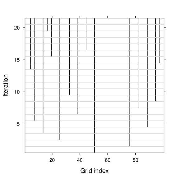
Some summaries and diagnostics of the result are listed in table 1. In the table one sees decisive increase in and decrease in mad ratios, as desired. Overall, the number of anchors started at 2 and increased to 16. Because the geostatistical parameter had 4 components, the dimension of the model parameter started at 6 and increased to 20. The adaptive nature of anchor selection in the algorithm is vividly depicted in figure 3, which shows the evolution of the anchorsets in the iterations.
| Iteration | Sample size | Anchors | Median | Max | |
|---|---|---|---|---|---|
| 1 | 2400 | 2 | -48.6 | 1.0000 | 1.000 |
| 2 | 1950 | 3 | -7.4 | 0.1829 | 0.346 |
| 3 | 1612 | 4 | 31.7 | 0.0354 | 0.188 |
| 4 | 1359 | 5 | 35.2 | 0.0402 | 0.146 |
| 5 | 1170 | 6 | 43.3 | 0.0290 | 0.138 |
| 6 | 1027 | 7 | 49.1 | 0.0270 | 0.086 |
| 7 | 920 | 8 | 72.9 | 0.0110 | 0.089 |
| 8 | 840 | 9 | 85.1 | 0.0081 | 0.063 |
| 9 | 780 | 10 | 84.0 | 0.0095 | 0.034 |
| 10 | 735 | 11 | 83.6 | 0.0091 | 0.034 |
| 11 | 701 | 11 | 70.0 | 0.0086 | 0.040 |
| 12 | 676 | 11 | 85.8 | 0.0096 | 0.025 |
| 13 | 657 | 11 | 90.4 | 0.0063 | 0.026 |
| 14 | 643 | 12 | 96.0 | 0.0064 | 0.022 |
| 15 | 632 | 13 | 99.2 | 0.0051 | 0.023 |
| 16 | 624 | 14 | 98.8 | 0.0052 | 0.021 |
| 17 | 618 | 15 | 103.3 | 0.0040 | 0.036 |
| 18 | 614 | 15 | 106.0 | 0.0037 | 0.037 |
| 19 | 610 | 15 | 101.5 | 0.0038 | 0.038 |
| 20 | 608 | 16 | 97.8 | 0.0037 | 0.038 |
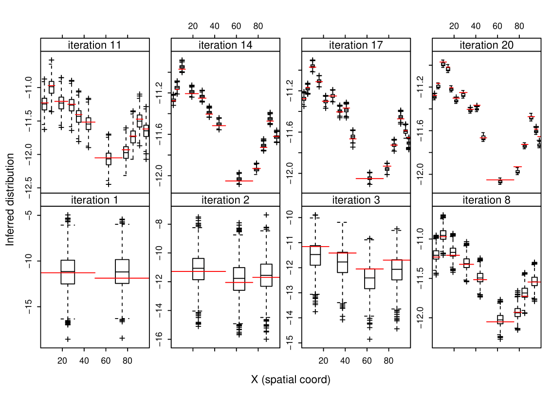
Figure 4 shows the inferred marginal distribution of each anchor, as represented by a boxplot of the sample obtained in step 1 of the algorithm. Since the anchorsets evolved in iterations, we do not see the “convergence” of the distribution of a fixed anchorset. Because the true field is known, each anchor has a “target value” defined by the true values. These target values are indicated in figure 4. It is seen that the estimated distributions homed in on the target values convincingly after a few iterations. This strength of convergence for a reasonably large number of anchors suggests that the parameterization provides a good presentation of the field.
The estimated marginal distributions of the geostatistical parameters are shown in figure 5. It should be stressed that the meaning of the geostatistical parameters changes during the iterations whenever the anchorset changes. In addition, interactions between the geostatistical parameters cause difficulty in their inference (see Zhang [2012]). Compared to the anchor parameters, the role of geostatistical parameters is more of an intermediate modeling device.
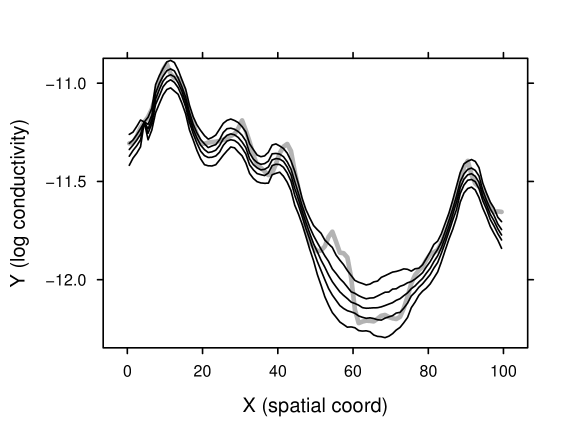
Recall that the goal of anchored inversion is to characterize the field . We created 1000 field realizations based on the anchorset and approximate posterior distribution in the final iteration (i.e. in this particular example). The 5th, 25th, 50th, 75th, and 95th percentiles of the realizations for each grid point are plotted in figure 6, overlaid with the synthetic field for comparison. The comparison confirms the inversion worked well.
In real-world applications, we do not know the true field, therefore can neither compare the field simulations with the truth nor compare the anchors with their target values. Perhaps the most concrete assessment is provided by the capabilities of simulated fields to “reproduce” the forward data. In each iteration of the algorithm, the sample obtained in step 2 represents “predictions” of the observation based on the posterior distribution estimated in the previous iteration. These predictions are compared with the actual observations in figure 7. In each panel (for one iteration), a vertical box-plot for each component of the predictions is drawn on the horizontal location where the observed value is. Therefore, if the predictions reproduce the observations, the box-plots should fall centered on the line. The figure demonstrates that the reproduction starts severely biased and outspread in the initial iteration and, after steady adjustment of the mean and reduction of the variance in subsequent iterations, achieves precise match with the actual observation in the final iterations.
7.4 Example 2: rainfall and surface runoff
Runoff over the land surface generated during and after a rainfall event is affected by the hydraulic roughness of the land surface [Vieux, 2004, chap 6]. By affecting runoff, the roughness also exerts important influence on infiltration, erosion, and vegetative growth. However, detailed measurement of the roughness coefficient in a watershed is impractical. In many hydrological and agricultural models, surface roughness is treated as a constant or as a categorical variable taking a few values based on the type of the land cover. Huang and Lee [2009] investigate the effect of spatially heterogeneous roughness on the runoff process. They consider a one-dimensional overland plane model described by the following equation system:
| (26) |
where is the spatial coordinate (m), is the time (s), is the flow depth (m), is the flow discharge per unit width (), is the effective rainfall (), is the friction slope (m/m), is the bed slope (m/m), is the flow velocity (), and is the Manning roughness coefficient (). In this system, the rainfall input and the bed slope are considered known. In addition, the initial condition and boundary condition are assumed. These conditions state that the surface is dry at the beginning of the rainfall event, and there is no inflow at the upstream boundary.
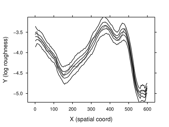
Whereas Huang and Lee [2009] investigate the resultant and under various configurations of synthetic roughness , we considered the inverse problem: infer the spatial field of given observations of and . The synthetic log-roughness field we used is shown in figure 8. The field consists of 150 grid points.
To make it more interesting, we constructed two synthetic rainfall events and corresponding observation scenarios. In the first event, rainfall lasted for 60 minutes with a uniform intensity of 5. The discharge at the downstream boundary was measured every 10 minutes for 3 hours (that is, during the rain and in the subsequent 120 minutes). In the second event, rainfall lasted for 30 minutes with a uniform intensity of 20. The flowdepth at the downstream boundary was measured every 5 minutes for 4 hours (that is, during the rain and in the subsequent 210 minutes). These two time-series datasets were combined to form a forward data vector of length 66. The discharge and flowdepth processes at the downstream boundary in the two rain events, computed based on the synthetic roughness field, are depicted in figure 9. We took and modeled as a Gaussian process. The forward function involved obtaining , solving the equation system (26) for and based on each of the two rainfall scenarios, extracting (or ) at the specified space and time coordinates, and taking the combined vector as the forward data . Note here the forward data contained some discharge measurements and some flowdepth measurements. These two physical quantities are of incomparable natures.
In the iterative algorithm, principal component analysis reduced the dimension of the forward data from 66 down to 9–19. Such significant dimension reduction was expected given the high level of auto-correlation in the time series data.
Performance of the inversion is demonstrated by 1000 field realizations created based on the final approximation to the posterior distribution of . Representative percentiles of the simulated realizations are shown in figure 10 with comparison to the synthetic field, confirming the potential of the inversion method.
7.5 Example 3: seismic tomography
The propagation of natural or man-made seismic waves through the earth is controlled by certain physical properties of the rock media along the path of the wave propagation. It is conventional to think of the media as constituting a “velocity field”, that is, each location is characterized by a velocity which is determined by relevant rock properties at that location. Suppose seismic P-wave emanates from a source location and is detected at a receiver location, where the “first-arrival traveltime” of the wave is recorded. The ray path (i.e. route of the wave propagation) is a complicated function of the velocity field; in particular, it is not a straight line where the velocity field is not uniform. The traveltime is determined by the velocities on the ray path from the source to the receiver. If one knows the velocity field, then both the ray path and the traveltime can be calculated [Vidale, 1988, 1990]. The inverse problem, namely inference of the velocity field given measurements of traveltimes, is called “seismic tomography”. First developed in medical imaging [Arridge, 1999], the tomography technique has seen wide applications in fields such as geophysics [Nolet, 2008] and hydrology [Yeh and Liu, 2000].
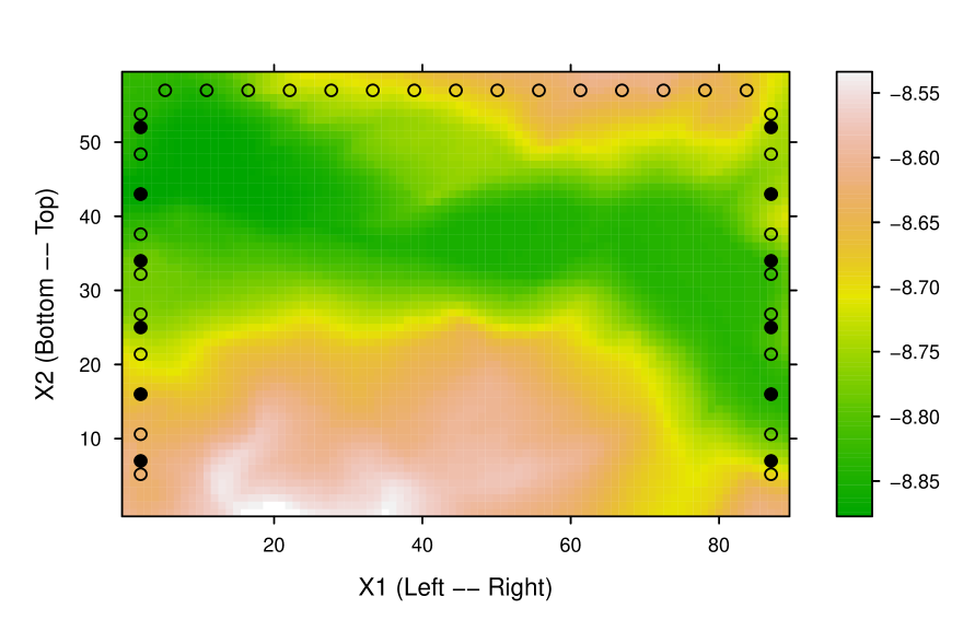
We constructed a synthetic tomography problem in two-dimensional space. Define “slowness” () as the reciprocal of velocity. Figure 11 shows a synthetic log-slowness () field (a vertical profile dipping down the ground surface), discretized into a grid. Suppose we conducted a tomography experiment with 6 sources and 10 receivers on each vertical boundary, and 15 receivers on the top boundary. Waves from each source were detected by the receivers on the opposite vertical boundary and on the top boundary. The sources and receivers are marked in figure 11. Such a layout of sources and receivers is typical of “crosshole tomography” [Ivansson, 1987, sec. 2.1].
The wave propagation is described approximately by the Eikonal equation [Shearer, 2009, Appendix C]:
| (27) |
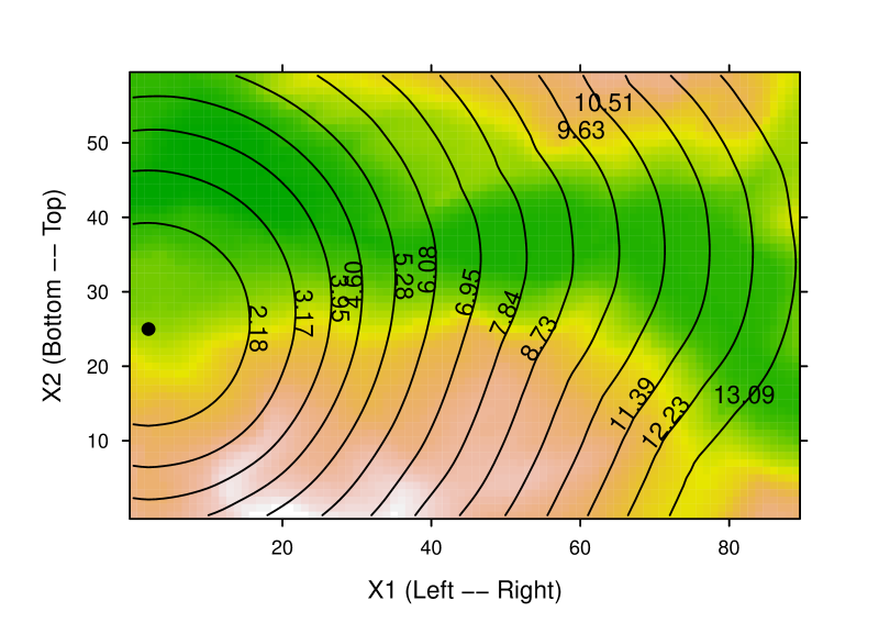
where , are the spatial coordinates, is the traveltime from a designated source to , and is the slowness at location . To illustrate a solution of this system, the contours of first-arrival traveltimes in the synthetic field from a source located on the left boundary are shown in figure 12. This figure clearly illustrates the curved paths of the seismic wave in the heterogeneous media. Note that the wave travels faster in regions of lower slowness (logically enough!).
Solving (27) in the synthetic slowness field and taking logarithmic transform of the resultant traveltimes, we obtained synthetic traveltime measurements. The solution used the algorithm described by Vidale [1988, 1990].
To reduce the computational cost, we aggregated the synthetic field into a grid, that is, a fourth of the resolution of the synthetic field. This introduces model error: the synthetic forward model and the forward model used in inversion are not identical—they use different numerical grids. This error is directly analogous to what discretization does to the conceptually continuous field in real-world applications. It may not be trivial to characterize this error quantitatively. In this example we chose to ignore this model error. Although in this particular case the error is small, the notion of ignoring the error is important in illustrating the principles of the anchored inversion methodology. In contrast, some other methods rely on the notion of “error” to construct regularization criteria or likelihood functions (see section 2).
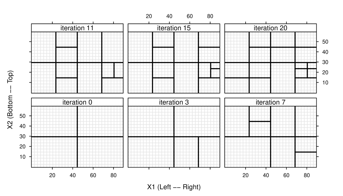
In the iterations of the algorithm, the dimension of the forward data was reduced from 300 to 25–107, thanks to the principal component analysis in step 3 of the algorithm. The algorithm started with 4 anchors, dividing the model domain into sub-domains. The parameterization evolved in the 20 iterations and arrived at an anchorset with 16 anchors, as depicted in figure 13, which once again illustrates the adaptive nature of the algorithm in terms of automatically selecting an anchorset.
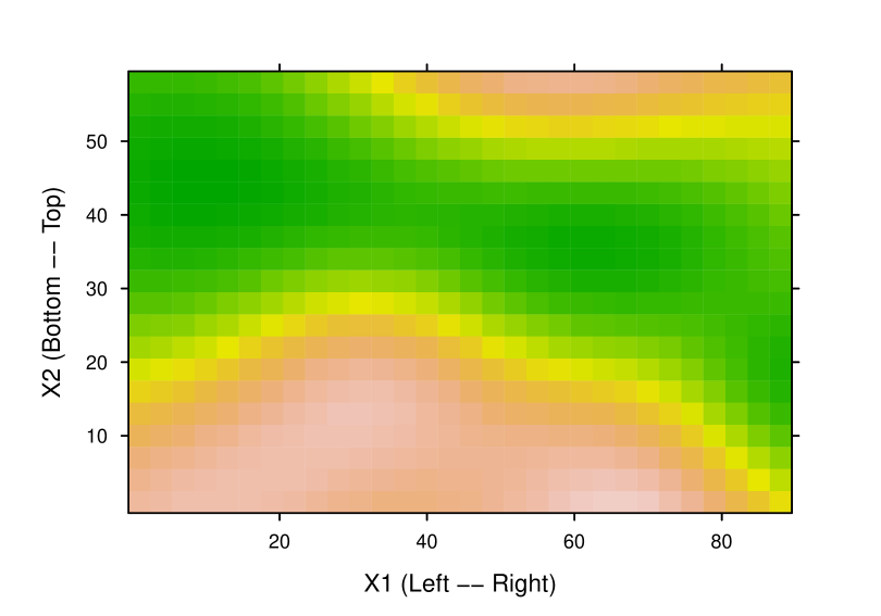
Based on the final approximation to the posterior distribution of the model parameter , we created 1000 field realizations (on the grid). The point-wise median of these realizations is shown in figure 14. Comparison with the synthetic field (aggregated to the grid) confirms that the inversion captured important features of the field. The mean of the point-wise standard deviations of the field realizations is 0.015, whereas the mean of the point-wise median absolute deviations (from the synthetic truth) is 0.036. These values should be considered with reference to the range of the synthetic field, which is .
8 Conclusion
We have proposed a general method for modeling a spatial random field, as a Gaussian process, that is tailored to making use of measurements of nonlinear functionals of the field. These nonlinear functionals are “forward processes (or models)” observed in experimental or natural settings. Inverse of nonlinear forward processes is a major topic with wide scientific applications, as demonstrated in sections 1 and 7.
The method revolves around certain deliberately chosen linear functionals of the field called “anchors”. The anchor parameterization achieves two goals. First, it reduces the dimensionality of the parameter space from that of the spatial field vector to that of the anchor vector (plus possibly a small number of other parameters such as geostatistical parameters). As a result, the dimensionality of the statistical inversion problem is separate from the spatial resolution of the forward model. Second, the parameterization establishes a statistical connection between the model parameter (i.e. anchors) and the data (i.e. forward process outcome). This statistical connection is known in mechanism and can be studied through simulations. The existence of this connection makes the inversion task a statistical one, whether or not the data contain model and measurement errors. This makes the method a fundamental departure from some existing approaches.
Although the framework has a Bayesian flavor, it does not go down a typical Bayesian computational path, because the likelihood function is unknown. The computational core lies in an iterative algorithm (section 4) centered on kernel density estimation. The algorithm is general and flexible in several aspects. First, it does not require a statistical analysis of the parameter-data connection, but only needs the ability to evaluate the forward model (usually by running a numerical code), which is treated as a black box operation. Although this study has focused on deterministic forward models, it is possible to accommodate stochastic ones. Second, the algorithm is flexible with regard to the prior specification. Third, the algorithm is able to accommodate flexible forms of errors (section 4.2). Fourth, different forward models (hence forward data) could be used in different iterations. The last point, not elaborated in this article, makes it possible to assimilate multiple datasets sequentially or in other flexible ways. These features make the algorithm a general procedure for approximating the posterior distribution where the likelihood is unknown but the model (which corresponds to the likelihood) can be simulated.
A critical component of the method concerns selecting the anchor parameterization in an adaptive, automatic fashion as iteration proceeds (section 5). The resultant anchor configuration is tailored to features of the field and the computational effort already invested. For example, if more iterations are performed, the algorithm in general will introduce more anchors to achieve more detailed representation of the field.
We used several synthetic examples to demonstrate a number of features of the methodology, including the capabilities of using linear data (example 1), using highly correlated data (all examples, especially examples 2 and 3), assimilating multiple datasets of different physical natures (example 2), and ignoring model or measurement errors (example 3). In view of the dimensionality of the parameter vector (in the tens) and that of the data (tens or hundreds), the algorithm showed potential in efficiency.
We have implemented the method in a R package named AnchoredInversion. Currently the package uses the packages RandomFields [Schlather, 2001] for simulating random fields and MASS (its function mvrnorm) [Venables and Ripley, 2002] for generating multivariate normal random numbers. The graphics in this article were created using the package lattice [Sarkar, 2008].
Acknowledgement: The work presented in this article was in part supported by the Excellent State Key Lab Fund no. 50823005, National Natural Science Foundation of China, and the R&D Special Fund for Public Welfare Industry no. 201001080, Chinese Ministry of Water Resources. The NED data (used in this study as synthetic data for the examples) from the National Map Seamless Server are open to the public, and are available from U.S. Geological Survey, EROS Data Center, Sioux Falls, South Dakota. Professor Paul Switzer suggested presenting the geostatistical parameterization as an extension (instead of being integrated from the beginning). The author thanks an anonymous reviewer for constructive comments.
References
- Aitkin [1991] M. Aitkin. Posterior Bayes factors. J. R. Stat. Soc., B, 53(1):111–142, 1991. URL http://www.jstor.org/stable/2345730.
- Arridge [1999] S. R. Arridge. Optical tomography in medical imaging. Inverse Problems, 15:R41–R93, 1999. doi: doi:10.1088/0266-5611/15/2/022.
- Besag et al. [1991] J. Besag, J. York, and A. Mollié. Bayesian image restoration, with two applications in spatial statistics. Ann. Inst. Statist. Math., 43(1):1–59, 1991.
- Beven [1993] K. Beven. Prophecy, reality and uncertainty in distributed hydrological modelling. Adv. Water Resour., 16:41–51, 1993.
- Bube and Burridge [1983] K. P. Bube and R. Burridge. The one-dimensional inverse problem of reflection seismology. SIAM Review, 25(4):497–559, 1983.
- Doherty [2003] J. Doherty. Ground water model calibration using pilot points and regularization. Ground Water, 41(2):170–177, 2003.
- Engl and Neubauer [2000] M. H. H. W. Engl and A. Neubauer. Regularization of Inverse Problems. Kluwer, 2000.
- George [2006] E. I. George. Bayesian model selection. In S. Kotz, C. B. Read, N. Balakrishnan, and B. Vidakovic, editors, Encyclopedia of Statistical Sciences. John Wiley & Sons, Inc., 2006.
- Geweke [1989] J. Geweke. Bayesian inference in econometric models using Monte Carlo integration. Econometrica, 57(6):1317–1339, 1989.
- Ginn and Cushman [1990] T. R. Ginn and J. H. Cushman. Inverse methods for subsurface flow: a critical review of stochastic techniques. Stoch. Hydrol. Hydraul., 4:1–26, 1990.
- Higdon [2002] D. Higdon. Space and space-time modeling using process convolutions. In Quantitative Methods for Current Environmental Issues, pages 37–56. Springer, 2002.
- Higdon et al. [2003] D. Higdon, H. Lee, and C. Holloman. Markov chain Monte Carlo-based approaches for inference in computationally intensive inverse problems. In Bayesian Statistics, volume 7. Oxford University Press, 2003.
- Huang and Lee [2009] J.-K. Huang and K. T. Lee. Influences of spatially heterogeneous roughness on flow hydrographs. Adv. Water Resour., 32:1580–1587, 2009.
- Ivansson [1987] S. Ivansson. Crosshole transmission tomography. In G. Nolet, editor, Seismic Tomography, pages 159–188. D. Reidel Publishing Company, 1987.
- Kaipio and Somersalo [2005] J. Kaipio and E. Somersalo. Statistical and Computational Inverse Problems. Applied Mathematical Sciences 160. Springer, 2005.
- Kass and Raftery [1995] R. E. Kass and A. E. Raftery. Bayes factors. J. Am. Stat. Assoc., 90(430):773–795, 1995.
- Kirsch [1996] A. Kirsch. An Introduction to the Mathematical Theory of Inverse Problems. Springer, 1996.
- Kravaris and Seinfeld [1985] C. Kravaris and J. H. Seinfeld. Identification of parameters in distributed parameter systems by regularization. SIAM J. Control Optim., 23(2):217–241, 1985.
- Lee et al. [2002] H. K. H. Lee, D. M. Higdon, Z. Bi, M. A. R. Ferreira, and M. West. Markov random field models for high-dimensional parameters in simultaitons of fluid flow in porous media. Technometrics, 44(3):230–241, 2002. doi: 10.1198/004017002188618419.
- Marjoram et al. [2003] P. Marjoram, J. Molitor, V. Plagnol, and S. Tavaré. Markov chain Monte Carlo without likelihoods. Proceedings of the National Academy of Sciences, 100:15324–15328, 2003. doi: 10.1073/pnas.0306899100.
- Marron and Wand [1992] J. S. Marron and M. P. Wand. Exact mean integrated squared error. Ann. Statist., 20(2):712–736, 1992.
- McLachlan [2000] G. McLachlan. Finite Mixture Models. John Wiley & Sons, Inc., 2000.
- Nakagiri [1993] S. Nakagiri. Review of Japanese work of the last ten years on identifiability in distributed parameter systems. Inverse Problems, 9:143–191, 1993.
- Newsam and Enting [1988] G. N. Newsam and I. G. Enting. Inverse problems in atmospheric constituent studies: I. determination of surface sources under a diffusive transport approximation. Inverse Problems, 4:1037–1054, 1988.
- Nolet [2008] G. Nolet. A Breviary of Seismic Tomography. Cambridge University Press, 2008.
- O’Sullivan [1986] F. O’Sullivan. A statistical perspective on ill-posed inverse problems. Statistical Science, 1(4):502–518, 1986.
- Owen and Zhou [2000] A. Owen and Y. Zhou. Safe and effective importance sampling. J. Am. Stat. Assoc., 95(449):135–143, 2000.
- Sambridge and Mosegaard [2002] M. Sambridge and K. Mosegaard. Monte Carlo methods in geophysical inverse problems. Reviews of Geophysics, 40(3), 2002. doi: 10.1029/2000RG000089.
- Sarkar [2008] D. Sarkar. Lattice: Multivariate Data Visualization with R. Springer, 2008.
- Scales and Tenorio [2001] J. A. Scales and L. Tenorio. Prior information and uncertainty in inverse problems. Geophysics, 66(2):389–397, 2001.
- Schlather [2001] M. Schlather. Simulation and analysis of random fields. R News, 1(2):18–20, June 2001.
- Schoups et al. [2010] G. Schoups, J. A. Vrugt, F. Fenicia, and N. C. van de Giesen. Corruption of accuracy and efficiency of Markov chain Monte Carlo simulation by inaccurate numerical implementation of conceptual hydrologic models. Water Resour. Res., 46:W10530, 2010. doi: 10.1029/2009WR008648.
- Schwartz and Zhang [2003] F. W. Schwartz and H. Zhang. Fundamentals of Ground Water. John Wiley & Sons, Inc., 2003.
- Shearer [2009] P. M. Shearer. Introduction to Seismology. Cambridge University Press, 2nd edition, 2009.
- Short et al. [2010] M. Short, D. Higdon, L. Guadagnini, A. Guadagnini, and D. M. Tartakovsky. Predicting vertical connectivity within an aquifer system. Bayesian Analysis, 5(3):557–582, 2010.
- Stein [1999] M. L. Stein. Interpolation of Spatial Data: Some Theory for Kriging. Springer, 1999.
- Tanner [1996] M. A. Tanner. Tools for Statistical Inference. Springer, 3rd edition, 1996.
- Tarantola [2005] A. Tarantola. Inverse Problem Theory and Methods for Model Parameter Estimation. SIAM, Philadelphia, 2005.
- Tarantola and Valette [1982] A. Tarantola and B. Valette. Inverse problems = question for information. Journal of Geophysics, 50:159–170, 1982.
- Tenorio [2001] L. Tenorio. Statistical regularization of inverse problems. SIAM Review, 43(2):347–366, 2001.
- Tikhonov and Arsenin [1977] A. Tikhonov and V. Arsenin. Solution of Ill-posed Problems. Winston, Washington, DC, 1977.
- van Leeuwen and Evensen [1996] P. J. van Leeuwen and G. Evensen. Data assimilation and inverse methods in terms of a probablistic formulation. Mon. Weather Rev., 124:2898–2913, 1996.
- Venables and Ripley [2002] W. N. Venables and B. D. Ripley. Modern Applied Statistics with S. Springer, 4th edition, 2002.
- Vidale [1988] J. Vidale. Finite-difference calculation of travel times. Bulletin of the Seismological Society of America, 78(6):2062–2076, 1988.
- Vidale [1990] J. E. Vidale. Finite-difference calculation of traveltimes in three dimensions. Geophysics, 55(5):521–526, 1990.
- Vieux [2004] B. E. Vieux. Distributed hydrologic modeling using GIS. Kluwer, 2nd edition, 2004.
- Welch and Bishop [1995] G. Welch and G. Bishop. An introduction to the Kalman filter. Technical Report TR 95-041, Department of Computer Science, University of North Carolina at Chapel Hill, 1995. Updated in 2006.
- West [1993] M. West. Approximating posterior distributions by mixture. J. R. Stat. Soc., B, 55(2):409–422, 1993.
- Yeh and Liu [2000] T.-C. J. Yeh and S. Liu. Hydraulic tomography: development of a new aquifer test method. Water Resour. Res., 36(8):2095–2105, 2000.
- Yeh [1986] W. W.-G. Yeh. Review of parameter identification procedures in groundwater hydrology: the inverse problem. Water Resour. Res., 22(2):95–108, 1986.
- Zhang [2012] Z. Zhang. Iterative posterior inference for Bayesian kriging. Stoch. Environ. Res. Risk Assess., 26(7):913–923, 2012. doi: 10.1007/s00477-011-0544-y.
- Zhang et al. [2007] Z. Zhang, D. Beletsky, D. J. Schwab, and M. L. Stein. Assimilation of current measurements into a circulation model of Lake Michigan. Water Resour. Res., 43:W11407, 2007. doi: 10.1029/2006WR005818.