Adaptive County Level COVID-19 Forecast Models: Analysis and Improvement
Abstract
Accurately forecasting county level COVID-19 confirmed cases is crucial to optimizing medical resources. Forecasting emerging outbreaks pose a particular challenge because many existing forecasting techniques learn from historical seasons trends. Recurrent neural networks (RNNs) with LSTM-based cells are a logical choice of model due to their ability to learn temporal dynamics. In this paper we adapt the state and county level influenza model, TDEFSI-LONLY, proposed in Wang et al. (2020) to national and county level COVID-19 data. We show that this model poorly forecasts the current pandemic. We analyze the two week ahead forecasting capabilities of the TDEFSI-LONLY model with combinations of regularization techniques. Effective training of the TDEFSI-LONLY model requires data augmentation, to overcome this challenge we utilize an SEIR model and present an inter-county mixing extension to this model to simulate sufficient training data. Further, we propose an alternate forecast model, County Level Epidemiological Inference Recurrent Network (CLEIR-Net) that trains an LSTM backbone on national confirmed cases to learn a low dimensional time pattern and utilizes a time distributed dense layer to learn individual county confirmed case changes each day for a two weeks forecast. We show that the best, worst, and median state forecasts made using CLEIR-Net model are respectively New York, South Carolina, and Montana.
1 Introduction
The ongoing novel COVID-19 pandemic has strained United States healthcare systems increasing the importance of optimizing medical resource allocation. This optimization will depend on the accuracy and precision of the models used to forecast confirmed cases in a given area W. Yang (2016); C. Doms (2018); C. Murray (2020b, a); S. Mehrotra (2020). To the best of our knowledge, current COVID-19 modeling literature primarily consists of two main approaches: SEIR modeling and Recurrent Neural Network (RNN) forecasting national trends for the purpose of determining transmission parameters and evaluating the effectiveness of national policies A.J. Kucharski (2020); Y. Fang (2020); J.T. Wu (2020); Coelho (2020); V. Reddy (2020); Dandekar and Barbastathis (2016). The SEIR model has a long history in epidemiology Kermack and McKendrick (1927) and the benefit of this model is the direct mathematical modeling of disease transmission which can be fit to known data as was seen at the outbreak in Wuhan A.J. Kucharski (2020); Y. Fang (2020); J.T. Wu (2020); C. Anastassopoulou (2020). The SEIR model is particularly useful for policy makers as the measurable constants that affect the transmission and disease dynamics can be easily monitored. Its vulnerability is its lack of complexity to represent the full range of the pandemics transmission dynamics. This becomes evident when forecasting at the county level in an interconnected region like the United States.
Recurrent Neural Networks (RNNs) are known to perform well when learning sequential patterns and are often applied to capture dynamic temporal behavior in time series. Similar to other types of deep networks, RNN training requires a large number of data to handle the high complexity associated with dimensionality. Possibly the largest challenge in forecasting COVID-19 is overcoming the curse of dimensionality with the limited data available. Here, there is simply not enough data to justify a complex model with millions of parameters and explanatory features. One solution is using simulated data from a deterministic epidemiological model to supplement real data. For simplicity of the process we may simulate epidemics using randomized but relevant parameter sets. The results are then used to train an RNN model.
We adapt a variant of an influenza epidemic forecast model, TDEFSI, proposed by Wang et al. (2020) to forecast the COVID-19 pandemic in county level. TDEFSI features a single branch RNN with two-stacked LSTM layers to capture the time pattern in the times series training data. The authors utilize the technique of data augmentation: the generation of SEIR simulated data to be used as training data. However, the standard SEIR models neglect migration to and from the modeled region which might change the proportion of the labeled populations. This is not a suitable assumption when modeling individual counties since cross county flows remain significant even under lockdowns in urban areas such as New York City due to their interconnection and close proximity. In our paper, this is amended by incorporating an inflow and outflow term into each labeled population’s Ordinary Differential Equation (ODE).
In this work, we propose a novel, state-of-the-art, architecture of RNN, County Level Epidemiological Inference Recurrent Network (CLEIR-Net), that requires fewer parameters, thereby mitigating overfitting, and, considerably improving both forecast error and training time. The approach reduces the number of parameters using a hierarchy of relationships to learn a mapping from a low dimensional, national level, signal to a high dimensional, county level, signal.
2 Related Work
From the onset of the pandemic epidemiologists began using deterministic SEIR modeling in Wuhan, China to estimate the basic reproductive number and forecast infections A.J. Kucharski (2020); Y. Fang (2020); J.T. Wu (2020); C. Anastassopoulou (2020). Several teams have used machine learning models to produce national forecasts of confirmed cases in Canada, Brazil, Wuhan, Italy, South Korea, and the United States, as found in Coelho (2020); V. Reddy (2020); Dandekar and Barbastathis (2016). During the writing of this paper we found Nicholas Soures (2020) used a combined LSTM network and SEIR architecture with mobility data to model county level confirmed cases for SEIR parameter estimation and measuring the effect of population mobility. At the time that we started this project there were no published models used to forecast high resolution county-level data for COVID-19 to date. This led us to adapt forecasting models used for other epidemics, specifically the TDEFSI, described in Wang et al. (2020).
Three variants of the TDEFSI models were developed to forecast influenza epidemics. Two of these utilize the two branch architecture and provide superior results. However, the models require previous seasons data to train making them unusable for the COVID-19 pandemic due to its novelty. The third variant is TDEFSI-LONLY with a one branch structure. This model along with proposed regularization terms were trained on SEIR simulated New Jersey data and outperformed LSTM[Hochreiter and Schmidhuber (1997)], AdapLSTM[S. Venna and Nichols (2019)]. The TDEFSI-LONLY model employs data augmentation, the generation of additional simulated data, for training at a higher resolution than exists in their datasets. This resolves the overfitting issue associated with deep neural networks that require many parameters. This paper’s application of data augmentation is to create an entirely simulated sample for training allowing the use of the real COVID-19 dataset for validation. In this study we explore the forecasting capability of the TDEFSI-LONLY model trained on SEIR generated data. We compare LONLY along with techniques found in Wang et al. (2020) and a dropout regularization technique Nitish Srivastava (2014) and Our new CLEIR-Net model overcomes some of the practical parameter training issues of LONLY method.
3 County Level Forecast Models
3.1 Adapted TDEFSI Model
In this section, we adapt the TDEFSI model proposed in Wang et al. (2020) to the COVID-19 forecasting problem. The the output of each step in the TDEFSI model has a dimension for each county, allowing the network to learn spatial relationships, without requiring knowledge of specific relationships beforehand. Let denote the sequence of the natural logs of daily nationwide incidence, where . Let denote the sequence of daily incidence for a particular county , where is the number of counties. Let . The objective is defined as predicting both nationwide and county-level incidence at day , where , denoted as . The TDEFSI loss function is given as:
| (1) |
where and are activity regularizers added to the outputs for spatial and non-negative consistency respectively, and and are penalty parameters. Since RNNs are not affected by the temporal scale of its input sequence, (1) does not need to be adjusted to account for the fact that COVID-19 data is updated daily as opposed to the weekly ILI data. Wang et al. (2020) only considered ILI data for individual states and their counties, whereas for COVID-19 we consider all counties in the nation. Min-max normalization is used on the county-level data so that . Whereas Wang et al. (2020) use the sum of for , here is the natural log of the sum of . This is done to normalize relative to while preserving the dependency of on . Without this normalization, would be significantly larger than any for a large , and would dominate the gradients used to optimize (1). This modification to requires that the regularization term be modified to be
| (2) |
In Section 4.1, we use simulated data from the county level adapted SEIR model Section 3.2 to supplement available real data and analyze the adapted TDEFSI model. We provide more details on the architecture of the model in Supplementary Material.
3.2 CLEIR-Net: Design Details
Notations and Parameters
Denote the number of counties, the number of features represented by the LSTM backbone, the number of dense units, LSTM cell state, the number of forecast, and the number of additional features. In our CLEIR-Net model we define a set of trainable parameters, , ,, , , , , and for the input, middle, and output layers of the County distributed dense layer , , ).
Description
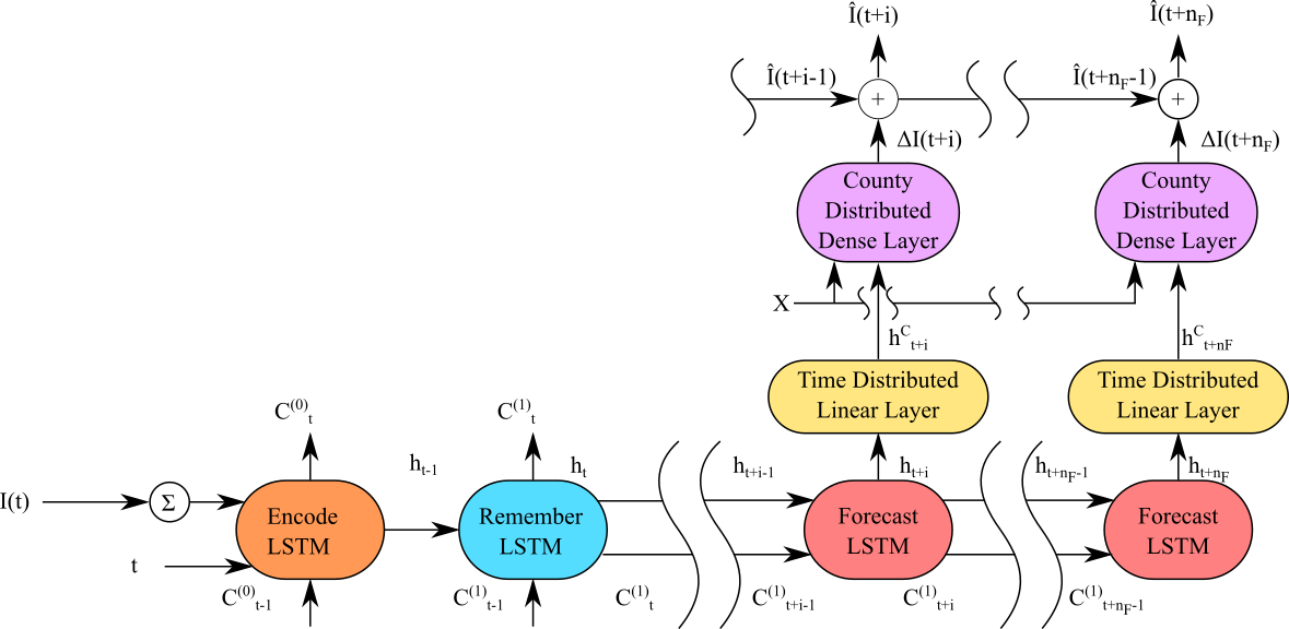
Our proposed CLEIR-Net architecture, Figure 1 is designed to both to minimize the number of trainable parameters and more closely align with underlying physical phenomenon than the TDEFSI architecture. The goal of CLEIR-Net is to learn to separate a high dimensional county level signal from a low dimensional national signal through a time dependent, time distributed, and county distributed hierarchy. The network is trained to encode complex national infection dynamics with a low dimensional time varying signal through an LSTM backbone when given the previous day’s national confirmed cases, days elapsed since the first national recorded case, and prior day’s LSTM cell state. Time invariant relationships are learned using a time distributed dense layer across all counties given the time pattern learned by the LSTM. County invariant relationships are then learned by a county distributed layer given each counties underlying time pattern and any additional county level features. Predictions from the county distributed layer are added to the previous day’s county level recorded cases to predict current day’s value. Using such a hierarchical representation allows us to expand the dimension of the input from the national to the county level without requiring a corresponding increase in parameters.
The architecture consists of an LSTM backbone, time distributed layer, and a county distributed layer. The LSTM backbone consists of an encode cell, remember cell, and, extendable forecast cell as shown in Figure 1. The encode cell is responsible for learning to incorporate the national total recorded cases and elapsed time into the backbone time pattern, given its past batch cell state. The remember cell is responsible for remembering forecasting cell’s state between batches, enabling longer term network memory without exposure to large gradients during backpropagation. The forecast cell is responsible for propagating the time pattern forward in time. Longer horizons can be forecast by repeating the forecast cell and using the preceding cell’s output as input to the next. For each step in time, the time distributed layer expands the low dimensional time features learned by the forecast cell into a high dimensional county level signal. Given the county level time feature and other county level features, the county distributed layer then learns to predict each counties change in confirmed cases.
To formulate the CLEIR-Net model, denote the function of a standard LSTM cell , linear dense layer , and nonlinear dense layer, where and are linear and non-linear activation functions. Now let be the number of days elapsed since the first recorded national confirmed case and let be the vector of true county level end of day confirmed cases. The encoder and remember LSTMs are given by:
| (3) |
where . Let be the index of the day in the forecast horizon. The extendable forecasting unit consists of a forecasting LSTM vertebrae, with a time distributed linear layer CLEIR-Net (Variant I), and with a combination of both time and county distributed layers CLEIR-Net (Variant II). The forecasting LSTM vertebrae is given by:
| (4) |
where is the time distributed linear layer and . Let be an additional county level feature matrix and let be the concatenation of with along the county axis, and let be the county index. The final layer predicts the change in each county’s confirmed cases given it’s current temporal feature through the following:
| (5) |
For , the forecast end of day recorded cases denoted by is then:
| (6) |
A detailed description of CLEIR-Net architecture is provided in the Supplementary Materials.
Spatial Mixing Extension to SEIR by Incorporating Inter-County Flow
The TDEFSI-LONLY model requires simulated training data supplemental to the JHU set used for testing. We trained using time series data generated using an inter-county population flow extended SEIR model similar to the model described in Bonnasse-Gahot et al. (2018). The full ODEs can be found in the supplementary material. For more compact form for efficient computation, let be the total number of counties. we denote total population of county , , Population with status in county , , where S, E, I, R stands for Susceptible (S), Exposed (E), Infected (I), Recovered (R) respectively. Let , and be total population flow of people from county to such that and for guaranteeing each county has no net change in population. . The matrix has the important property that , guaranteeing the conservation laws are satisfied. Then we have the following system of ODEs
| (10) |
is then solved for iteratively using Euler’s method, see Biswas et al. (2013), using , where is learning parameters. Next, assume that and , where is the spatial distance between to , is the population density of , and, , are the resistances to population flow, and infection spread respectively. The system is then controlled by the four parameters, , , , and the initial conditions, which are estimated as follows
| (13) |
Where and represent the prevalence of exposure in the susceptible population, and the prevalence of infection in the exposed population at time zero, respectively. A detailed breakdown explanation of each equation is included in the Supplementary Materials.
4 Experimental Results
COVID-19 Dataset
The dataset featured is JHU confirmed cases data for US counties which is updated daily. It provided a time series of confirmed cases from 1/22/20 to 5/31/20 along with latitude and longitudinal information for each county. We use this data or a subset of this data as a single sample for the adapted TDEFSI and CLEIR-Net. Note, due to limited testing capability in the US these confirmed cases numbers are the lower bound of the actual number of infections. This paper is forecasting the number of recorded cases, rather than infections.
4.1 Evaluation of Adapted TDEFSI Model
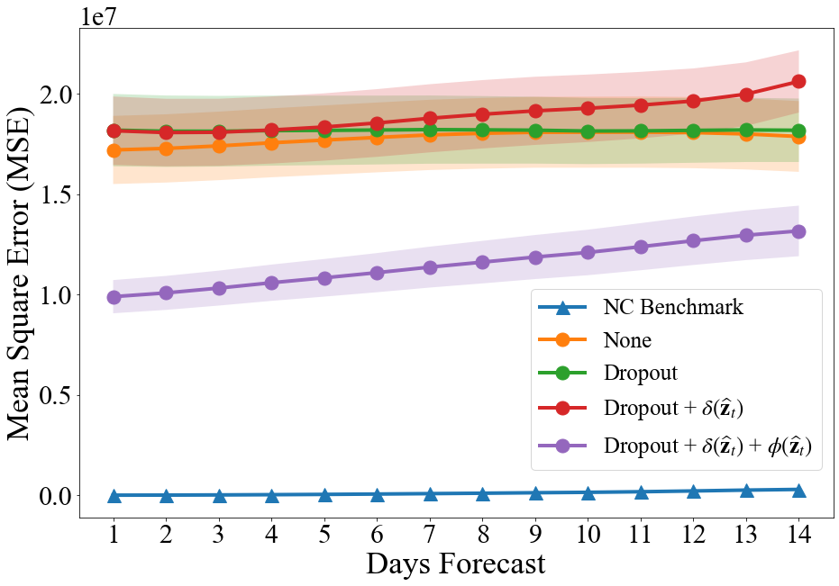
A total of 1024 SEIR simulations as described in Section 3.2 were run to train the adapted TDEFSI-LONLY model as described in Section 3.1, with an additional 16 simulations for validation. The network was trained for 300 epochs with a patience of 50. Four experiments were run: without any regularization, with dropouts, non-negative constraint regularization, and spacial consistency regularization. The final losses and MSE for each experiment are reported in Table 1. We provide the detailed list of parameters and number of hidden layers in the Supplementary Materials.
| None | Dropout | Dropout + | Dropout + + | |
|---|---|---|---|---|
| Train MSE | 2.57178e-5 | 5.24136e-5 | 1.54713e-4 | 2.444813e-4 |
| Valid MSE | 2.50214e-5 | 2.83442e-5 | 6.43349e-5 | 9.341941e-5 |
| Train Loss | - | - | 1.75519e-4 | 5.094754e-4 |
| Valid Loss | - | - | 8.26531e-5 | 1.906986e-4 |
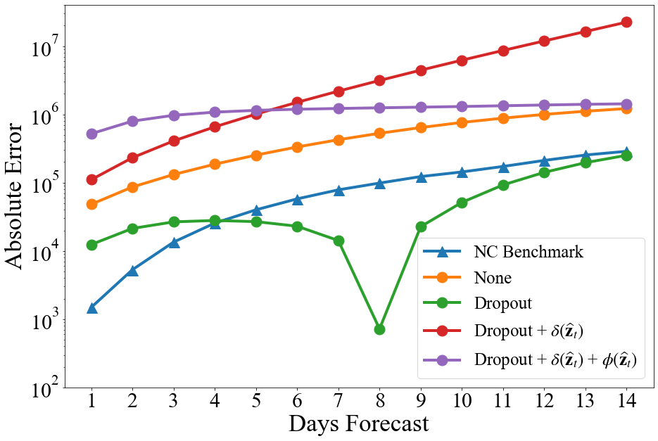
Figure 2a shows the MSE of for each day in the forecasts for 5/18/20 to 5/31/20 based on from 1/22/20 to 5/17/20 made using the adapted TDFESI networks, and Figure 2b shows the absolute error of for each day in that forecast.
4.2 CLEIR-Net Forecast Results
The model is trained with features from the 1/22/20 to 5/2/20 period, targets from 1/23/20 to 5/16/20 with validation features from 5/3/20 to 5/4/20 and targets from 5/3/20 to 5/17/20. The trained model is tested by making a single 14 day forecast over 5/18/20 to 5/31/20 for all counties. The county level temporal patterns are supplemented with standard normalized county level , , , and Killeen et al. (2020), as well as and prior to the application of the county distributed dense layer. We represent features in the LSTM backbone and use 3 layers of units in the county distributed branch taking to be the ReLU activation. Both training and inference use batch size of 1, with batches taken in sequential order, and previous encoding cell state shared with the next batch. Each batch uses the vector of the previous end of day’s recorded confirmed cases to forecast a target matrix of size . Dropout is applied to the targets at a rate of during training to mitigate overfitting.
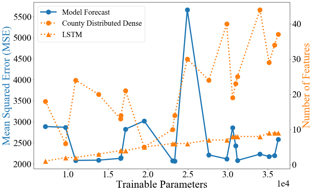
We perform a capacity study 2 by randomly sampling 20 configurations from with equal probability. While there is no clear trend in forecast mean squared error; we observe that a network with is reproducible and lightweight. Anecdotally, training proceeds best on the edge of instability, encouraging annealing of the network towards more stable configurations. Different size networks learn in different regimes, and capacity must be tuned in conjunction with dropout rate. We note that sharing cell state between sequential batches is essential for network convergence to an effective forecasting configuration. Using both the time distributed and county distributed dense layers is substantially more effective than using only a time distributed, or a time distributed, county distributed layer. Additionally, predictions from all 20 model configurations are ensembled by averaging and scored over the forecast horizon. The ensembled predictions perform better than any single model’s predictions, even in the presence of poor scoring component models. Due to the lightweight nature of of the architecture, ensembled predictions are easily obtained, mitigating the instability inherent in dropout and common in RNN architectures.
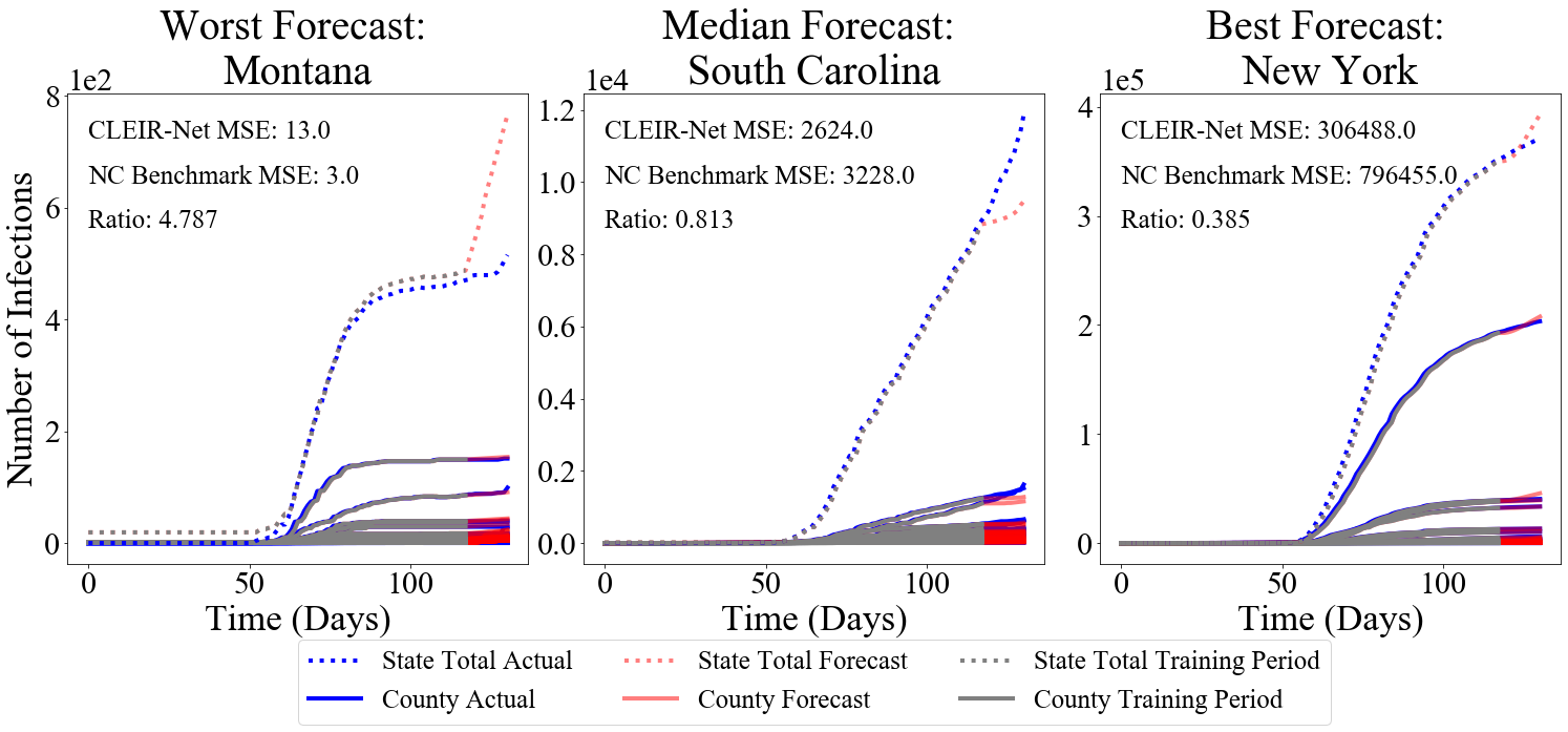
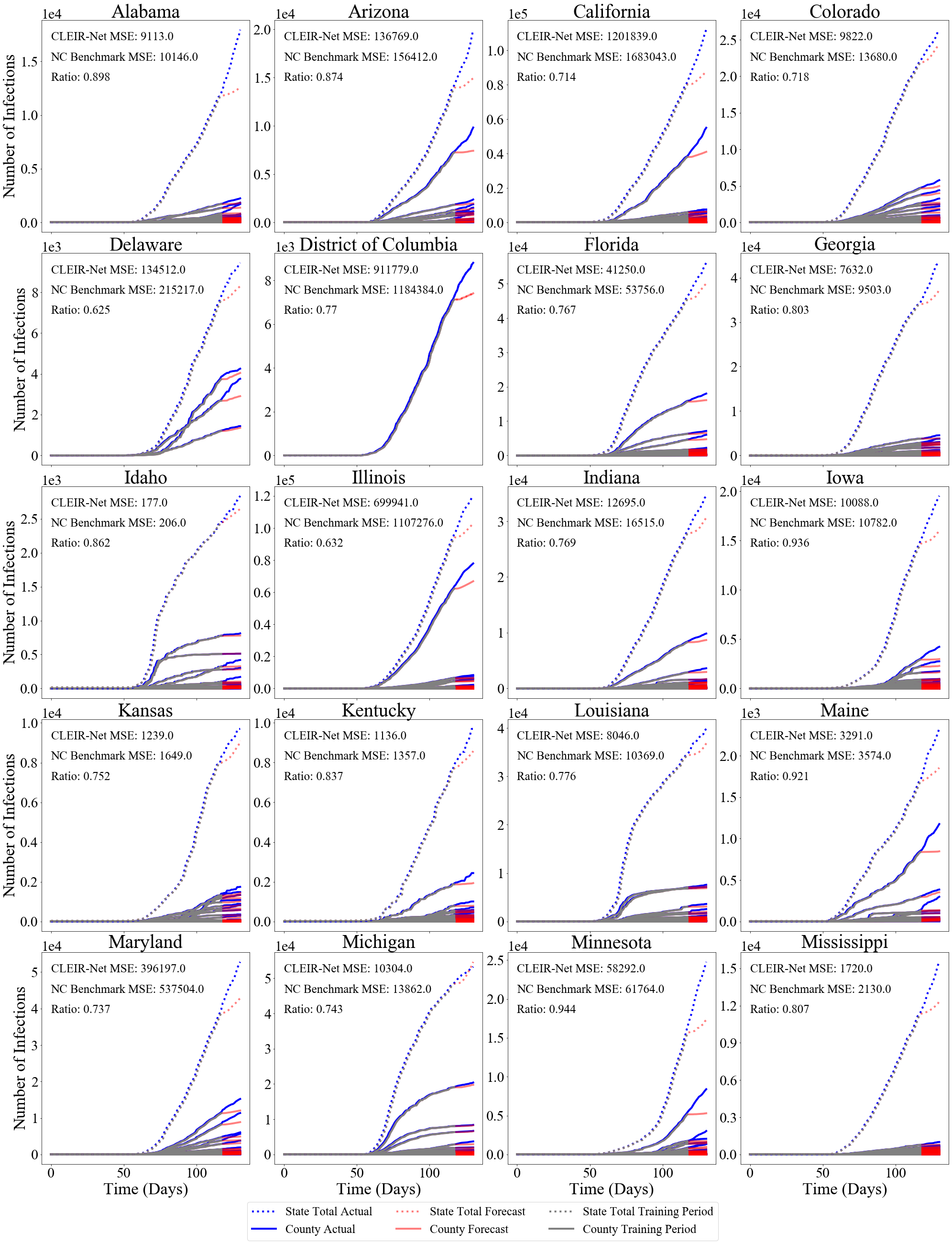
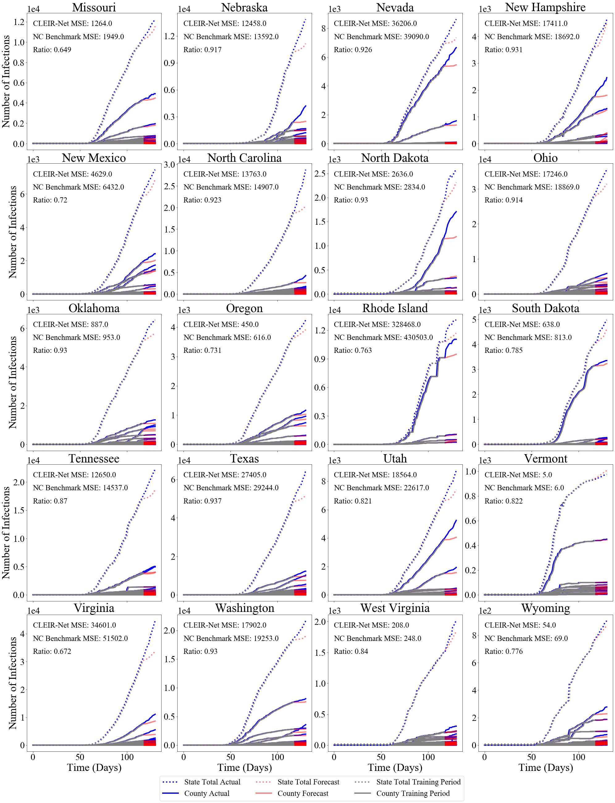
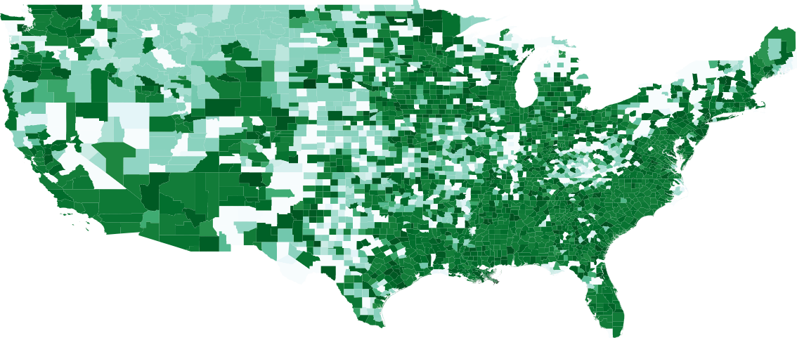
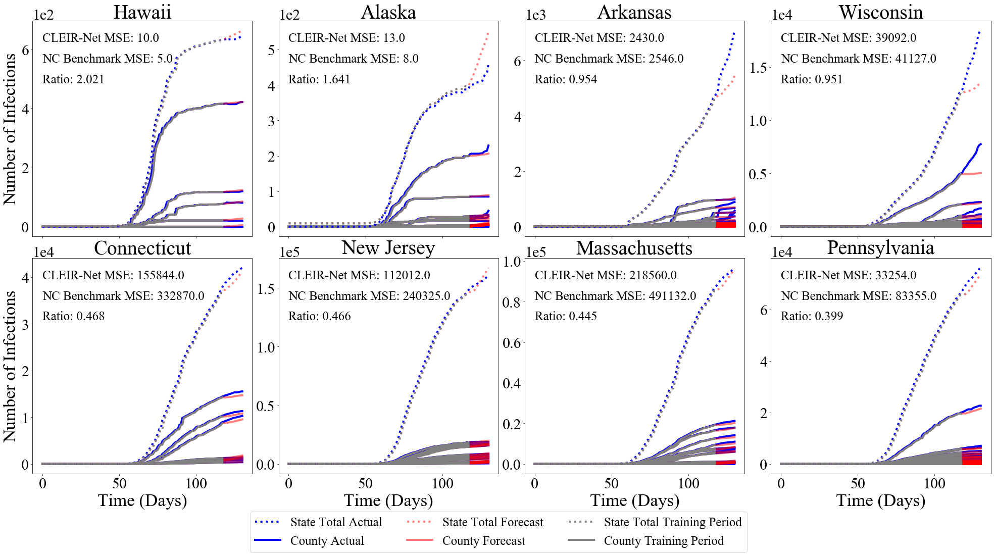
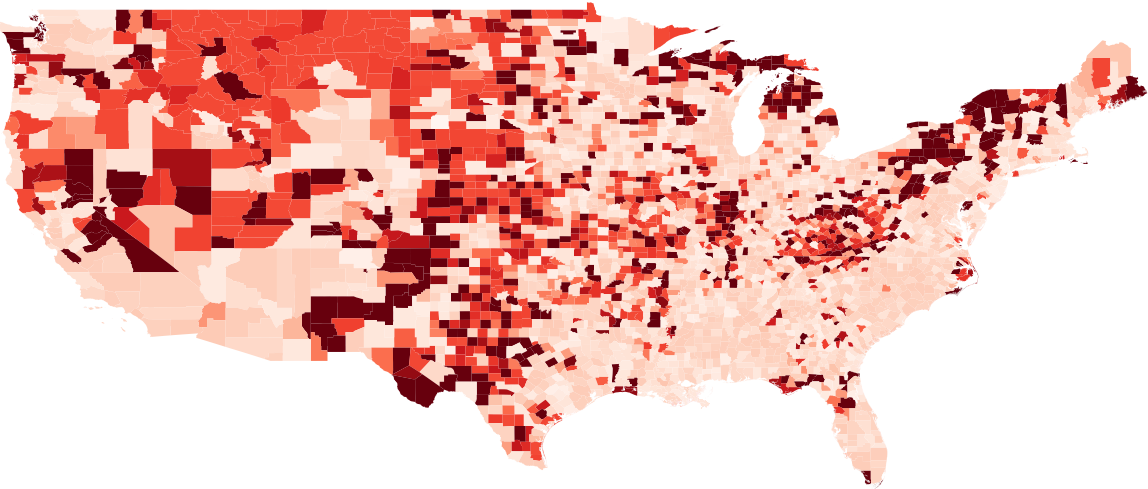
The best and worst performing model forecasts are collected in Figure 4. Figure 6 shows the second through fourth worst and the forth through second best forecasts made using CLEIR-Net model. Additional forecasts are provided in the Supplementary Material. Best predicted by CLEIR-Net are large, connected, counties. In particular, the top five best scoring state forecasts were the New York and four adjacent states: Pennsylvania, Massachusetts, New Jersey, and Connecticut. Worst predicted are small or isolated counties, such as Hawaii, and Montana. Also, poorly predicted are states with peculiar dynamics relative to the rest of the nation. For example, the five best predicted states exhibit the early stages of curve flattening, while Arkansas, and Wisconsin, the fourth and fifth worst predictions have an accelerating number of cases. Figure 5 illustrates this via a map showing the MSE for the contiguous states.
A summary of the forecast performance and size of all the models explored in this paper is presented in Table 2. All methods were used to forecast for 5/18/20 to 5/31/20. We observe that CLEIR-Net requires significantly low numbers of parameter to train versus the adapted TDFESI model.
| Model | Variant | MSE | Total Parameters |
|---|---|---|---|
| Benchmark | Naïve No Change | 108276 | - |
| CLEIR-Net | Average Ensemble of 20 | 69870 | - |
| Best Scoring | 70905 | 10945 | |
| Median Scoring | 75707 | 35847 | |
| Worst Scoring | 188677 | 24923 | |
| TDFESI | None | 17798679 | 1038405 |
| Dropout | 18178904 | 1038405 | |
| Dropout + | 18950460 | 1038405 | |
| Dropout + + | 11495507 | 1038405 |
5 Discussion
As expected, adding regularization terms to the loss function of the TDEFSI model increased the final loss and MSE, see Table 1. However, regularization did improve the generalization of the model, making it less likely to overfit the simulated training data. As seen in Figure 2a, combining the regularization methods improved the model’s county level forecasting performance, but underperforms the naïve no-change benchmark. The dropout method was the only regularization technique to improve the national forecasting performance, even outperforming the naïve no-change benchmark when forecasting more than four days out. While the TDEFSI model is viable for ILI forecasts as shown by Wang et al. (2020), the minor adaptations to the TDEFSI model tested here were insufficient to make the model a viable method for forecasting COVID-19 confirmed case data. More extreme adaptations or altogether different architectures, such as CLEIR-Net, must be considered.
There are many patterns superimposed on top of underlying pandemic dynamics, such as state, national, and temporal variations in policies for social distancing. This requires the careful balancing of capacity to fit complex observations without overfitting. CLEIR-Net is lightweight and scalable in terms of features and targets due to its hierarchical construction. While the number of features used by the LSTM backbone should be kept low since the time distributed has weights of shape future constructions might rethink this step. Further, there is likely room to learn stronger signals from appropriate features with existing capacity. Naturally, we should seek the smallest set of features for the neural network with the most explanatory power. This could be through the addition of mobility or policy data.
Limitations and Future Work
There are several experiments we wish to see explored. These models national forecasts could be improved through optimizing the SEIR model parameters. The sampling ranges of SEIR parameters could be extended to allow more diversity of simulation to ensure we do not restrict the model’s ability to capture all of the observed patterns. Future work on CLEIR-Net could consider improving the realism of the model and the connection of the network with underlying dynamics, such as by incorporating SEIR mechanics. Additional county level features might be incorporated at the county distributed layer. This same work could be done with the models trained on JHU global confirmed cases. In this case the countries would take the place of the counties in the current models and a world forecast would take the place of the national forecast in the current models. Additional work could be done to apply these methods to other measures of epidemiological progression, such as hospitalizations, death, and recovery rate.
6 Broader Impact
Two critical steps in the medical resource supply chain are procurement and deployment. For each, decision makers require their own specialized forecasting tools. The power of the proposed CLEIR-Net architecture is it’s ability to forecast over a large area concurrently at a higher resolution and for less computational expense than existing models. The model can give healthcare administrators in charge of medical resource allocation a two week lead time to optimize nationwide resource deployment to areas with the highest need and save lives. Meanwhile, many existing models, which are simpler and less computationally expensive, are sufficient to forecast single dimension national or regional pandemic dynamics and can reliably do so over longer horizons than two weeks to the benefit of system administrators in charge of procurement who must predict national and regional resource demand.
7 Acknowledgement
The authors would like to thank John Brindley, Mohsen Alizadeh Noghani, and Jens Early Hansen for their contribution to primary results established during the course “COS598 - Machine Learning” at University of Maine.
References
- A.J. Kucharski [2020] C. Diamond Y. Liu J. Edmunds S. Funk R.M. Eggo F. Sun M. Jit J.D. Munday et al. A.J. Kucharski, T.W. Russell. Early dynamics of transmission and control of COVID-19: a mathematical modelling study. Wiley, 2020. doi: 0.1016/S1473-3099(20)30144-4.
- Biswas et al. [2013] B N Biswas, Somnath Chatterjee, S Mukherjee, and Subhradeep Pal. A discussion on euler method: A review. Electronic Journal of Mathematical Analysis and Applications, 1:294–317, 06 2013.
- Bonnasse-Gahot et al. [2018] Laurent Bonnasse-Gahot, Henri Berestycki, Marie-Aude Depuiset, Mirta B Gordon, Sebastian Roché, Nancy Rodriguez, and Jean-Pierre Nadal. Epidemiological modelling of the 2005 french riots: a spreading wave and the role of contagion. Scientific reports, 8(1):1–20, 2018.
- C. Anastassopoulou [2020] A. Tsakris C. Siettos C. Anastassopoulou, L. Russo. Data-based analysis, modelling and forecasting of the covid-19 outbreak. PLoS ONE, 15(3), 2020.
- C. Doms [2018] J. Shaman C. Doms, S.C. Kramer. Assessing the use of influenza forecasts and epidemiological modeling in public health decision making in the united states. Scientific Reports, 8, 2018.
- C. Murray [2020a] IHME COVID-19 health service utilization forecasting team C. Murray. Forecasting the impact of the first wave of the covid-19 pandemic on hospital demand and deaths for the usa and european economic area countries. medRxiv, 2020a. URL https://doi.org/10.1101/2020.04.21.20074732.
- C. Murray [2020b] IHME COVID-19 health service utilization forecasting team C. Murray. Forecasting covid-19 impact on hospital bed-days, icu-days, ventilator-days and deaths by us state in the next 4 months. medRxiv, 2020b. URL https://doi.org/10.1101/2020.03.27.20043752.
- Coelho [2020] M. Ribeiroab R. Silva V. Mariani L. Coelho. Short-term forecasting covid-19 cumulative confirmed cases: Perspectives for brazil. Chaos, Solitons & Fractals, 2020. doi: https://doi-org.wv-o-ursus-proxy02.ursus.maine.edu/10.1016/j.chaos.2020.109853.
- Dandekar and Barbastathis [2016] R. Dandekar and G. Barbastathis. Quantifying the effect of quarantine control in covid-19 infectious spread using machine learning. medRxiv, 2016. doi: https://doi.org/10.1101/2020.04.03.20052084.
- Hochreiter and Schmidhuber [1997] S. Hochreiter and J. Schmidhuber. Long short-term memory. Neural Computation, 9:1735–1780, 1997.
- J.T. Wu [2020] G.M. Leung J.T. Wu, K. Leung. Nowcasting and forecasting the potential domestic and international spread of the 2019-ncov outbreak originating in wuhan, china: a modelling study. The Lancet, 395(10225):689–697, 2020.
- Kermack and McKendrick [1927] W. 0. Kermack and A. G. McKendrick. A contribution to the mathematical theory of epidemics. Proceedings of the Royal Society, Biological Sciences, 115:700–721, 1927.
- Killeen et al. [2020] Benjamin D. Killeen, Jie Ying Wu, Kinjal Shah, Anna Zapaishchykova, Philipp Nikutta, Aniruddha Tamhane, Shreya Chakraborty, Jinchi Wei, Tiger Gao, Mareike Thies, and Mathias Unberath. A county-level dataset for informing the united states’ response to covid-19, 2020.
- Nicholas Soures [2020] Zachariah Carmichael Anurag Daram Dimpy P. Shah Kal Clark Lloyd Potter Dhireesha Kudithipudi Nicholas Soures, David Chambers. Sirnet: Understanding social distancing measures with hybrid neural network model for covid-19 infectious spread. MATRIX-AI Consortium, 2020.
- Nitish Srivastava [2014] Alex Krizhevsky Ilya Sutskever Ruslan Salakhutdinov Nitish Srivastava, Geoffrey Hinton. Dropout: A simple way to prevent neural networks from over?tting. In Journal of Machine Learning Research 15, 2014.
- Noshad et al. [2018] M. Noshad, Y. Zeng, and A.O Hero. Scalable mutual information estimation using dependence graphs. Available on arXiv: 1801.09125, 2018.
- S. Mehrotra [2020] M. Barah F. Luo K. Schantz S. Mehrotra, H. Rahimian. A model of supply-chain decisions for resource sharing with an application to ventilator allocation to combat covid-19. Naval Research Logistics, 2020. doi: 10.1002/nav.21905.
- S. Venna and Nichols [2019] R. Gottumukkala V. Raghavan A. Maida S. Venna, A. Tavanaei and S. Nichols. A novel data-driven model for real-time influenza forecasting. IEEE Access, 7:7691–7701, 2019.
- V. Reddy [2020] L. Zhang V. Reddy. Time series forecasting of covid-19 transmission in canada using lstm networks. Chaos, Solitons & Fractals, 135, 2020. doi: https://doi.org/10.1016/j.chaos.2020.109864.
- W. Yang [2016] J. Shaman W. Yang, D.R. Olson. Forecasting influenza outbreaks in boroughs and neighborhoods of new york city. Public Library Of Science, 12, 2016.
- Wang et al. [2020] L. Wang, J. Chen, and M. Marathe. Tdefsi: Theory guided deep learning based epidemic forecasting with synthetic information. Available on arXiv: 2002.04663, 2020.
- Y. Fang [2020] M. Penny Y. Fang, Y. Nie. Transmission dynamics of the covid-19 outbreak and effectiveness of government interventions: A data-driven analysis. Journel of Medical Virology, 92:645–659, 2020.
Supplementary Materials
1 Spatial mixing Extension to SEIR
1.1 The SEIR model
The SEIR model assigns one of four status to a proportion of the total population in a space with constant population. It then builds a set of ordinary differential equations (ODEs) which describe rate of change of each status population. We use a version of the SEIR model that neglects birth and death effects and assumes a lack of any vaccination though it assumes recovered patients gain permanent resistance. The model is identical to one found in Y. Fang [2020] which is recreated below.
| (16) |
We denote to be the total population of county , and to be the population with status in county , where . is the proportion of the population with status . The parameters, , , and , along with initial conditions govern the dynamics of the epidemic. This model does not account for any interaction between the given county’s population and all other U.S. counties.
1.2 County Mixing SEIR Derivation
A conservation law for the population of the county requires the rate of population accumulation to equal the rate of population inflow minus the rate of population outflow plus the rate of population generation. The population generation term is given by our SEIR equations. We assume no change in the county population requiring the population flow and generation terms to add to zero. Additionally, intuitively we know the SEIR equations which govern the transition of status should not induce population accumulation or depreciation. This requires our population flow terms to balance.
We decided on population mixing terms that would account for the change in a status’ proportion of the population without changing the total county population. To do this, the inflow term for given population in county is a foreign county’s population flow into county multiplied by the foreign county’s proportion of population with status summed over all foreign counties. Symmetrically, the outflow term is the same population flow variable, but this time multiplied by proportion of population with status in county summed over each foreign county. The multiplication of the proportions, which must sum to one, and the flow terms, which are equivalent across ODEs for a county pair, ensure the county population does not change.
Let be the total population flow of people from county to such that and . These conditions guarantee each county has no net change in population. The derivatives of , can be written as
| (21) |
We can write this system of equations more concisely if we vectorize each equation. This can be done by creating a flow matrix, . The elements are made up of the aforementioned terms. Again, using the constraints and we create a symmetric flow matrix with a diagonal of zeros. Here, the th column represents population outflows from county and the th row represents population inflows to county . Lastly, we need our matrix to satisfy our constant population constraint. In other words, we want the diagonals of the matrix to be the negative sum of the other elements in their row. This can be done by subtracting the diagonal of one transpose , written as . This matrix exhibits the property , guaranteeing the conservation laws are satisfied.
2 Discussion on CLEIR-Net Model
2.1 CLEIR-Net Training
The network is trained over a sequence of inputs where the target is to forecast the number of recorded infections for each county for each of the next days in the future, given the days elapsed since the first national recorded infection, , the vector of the current day’s county level recorded infections, , and, crucially, the time invariant county level features, latitude, longitude, population, population density, log of population and population density. A batch size of one is used where each sample consists of a single given day of the pandemic and the corresponding targets are the days in it’s forecast horizon. That is, a sequence of overlapping samples, taken in sequential order. Additionally, each batch’s encoder and remember cells use the cell and hidden states from the previous batch’s encoder and remember cells as their initial states and provide their output states to the next sample’s corresponding cells. Sharing states between batches allows the LSTM cell to effectively utilize its memory property over the entire sequence but limit gradient exposure to short sequences. An initial state of zero is used for the first sample in the sequence.
2.2 CLEIR-Net Forecasting
After training, learned weights are used to forecast future infection trajectories. Since the model learns to use states from past batches, effective inference requires the model be initialized, post learning and prior to forecasting, by making sequential predictions over the entire training data.
2.3 CLEIR-Net Components
The network’s basic definitions, inputs, targets, and outputs for a single batch are summarized here.
Definitions
-
•
Number of days in the forecast horizon
-
•
Number of time features to model in the LSTM backbone
-
•
Number of counties in the prediction space
-
•
Number of additional county level features used by the county distributed dense layer
-
•
Number of units in the county distributed dense layer
Inputs:
-
•
: Time elapsed in days since first nationally recorded infection
-
•
: Current day’s county level infections
-
•
: Time invariant county level features
-
•
: State of the previous batch’s encoder cell
-
•
: State of the current batch’s encoder cell
-
•
: State of the previous batch’s remember cell
-
•
: State of the current batch’s remember cell
Targets:
The goal of the network is to forecast the end of day recorded infections for each US county for each day in the forecast horizon, therefore our targets are the following.
-
•
: Actual end of day recorded county level infections for the day in the forecast horizon.
Outputs: The corresponding model predicted infections are then denoted by the following.
-
•
: Predicted end of day county level infections for the day in the forecast horizon.
Additionally, each batch share’s the hidden and cell states of it’s encoder and remember LSTMs with the following batch.
-
•
: Cell state of the current batch’s encoder cell
-
•
: Hidden state of the current batch’s encoder cell
-
•
: Cell state of the current batch’s remember cell
-
•
: Hidden state of the current batch’s remember cell
The LSTM backbone of the model consists of an encoder cell and remember cell which translate the national total recorded infections and days elapsed into a low dimensional time varying pattern, and a repeatable forecast cell which propagates the time pattern into the future.
Encoder Cell:
-
•
Purpose: The encoder cell, given the previous batch’s encoder state, transforms the total national recorded infections, , and days elapsed since the first nationally recorded infection into a low dimensional time varying pattern.
-
•
Inputs: , , ,
-
•
Outputs: ,
-
•
Parameters: ,
Remember Cell:
-
•
Purpose: The remember cell, given the context from it’s previous state, and the output representation from the encoder, learns to remember the current state of the LSTM backbone used by the repeated forecast cell.
-
•
Inputs: , ,
-
•
Outputs: ,
-
•
Parameters: ,,
Forecast Cell:
-
•
Purpose: The forecast cell is similar to the remember cell in that its function is to model the underlying low dimensional time pattern. However, while the remember cell incorporates information both from the encoder cell and its own previous state, the forecast cell uses only the LSTM backbone state. For the first day in the forecast, the cell propagates the current state from the remember cell into the future. To achieve multiple days in the forecast horizon, the forecast cell is repeated, with each consecutive cell after the first taking the state from the previous cell as input.
-
•
Inputs: , when , , otherwise
-
•
Outputs: ,
-
•
Parameters: , ,
The time and county distributed layers are used to enforce a hierarchical framework of shared factors. The time distributed layer uses the same parameters across all time steps to learn a time pattern underlying each county, given the low dimensional patterns from the backbone. Then, given the underlying time pattern for each county, the county distributed layer predicts the day to day change in infections using the same set of explanatory factors shared by each county.
Time Distributed Layer:
-
•
Purpose: If we consider the low dimensional time pattern learned by the LSTM backbone to be a mixed signal representing the underlying national dynamics, then the goal of the time distributed linear layer is to separate the national time pattern into its county level components, providing a county level time dependent condition on which the county distributed layer is applied.
-
•
Inputs:
-
•
Outputs:
-
•
Parameters: ,
County Distributed Layer:
-
•
Purpose: Given descriptive factors comparable across counties, latitude, longitude, population, population density, and log population and population density, and the county level time feature learned by the time distributed layer, the county distributed layer predicts the county level daily changes in infections for all counties, .
-
•
Inputs: ,
-
•
Outputs:
-
•
Parameters: , , ) (For the input, hidden, and output layers of the County distributed dense layer.)
Final Prediction:
-
•
Purpose: The predicted changes in infection, , are added to the previous day’s predicted county level infections, , to determine the current day’s predicted infections, .
-
•
Inputs: , and when , or otherwise
-
•
Outputs:
-
•
Parameters None
3 Experimental Setup
3.1 CLEIR-Net Forecast
Network parameters are optimized by minimizing the weighted mean squared error (MSE) between the forecast and target matrices with NAdam with a learning rate of 0.001. Each sample is weighted by a factor of , where is the target number of days ahead in the forecast, and is the county. Training is stopped when the validation loss is unimproved for 30 epochs at which point weights from the best performing epoch are used for inference. Random dropout is applied to the targets during training at a rate of 0.25 to mitigate overfitting to any particular county’s patterns. Light L1 and L2 regularization of 0.00005 are applied to the kernel and bias weights of all dense layers and to all recurrent weights to improve conditioning of the gradient. Forecasting is performed using learned parameters by resetting cell states and making predictions with a batch size of one in sequential order over all available days in the input range; ensuring the memory property is active during inference. Predictions from the last available day are taken as the forecast.
Prior to training, 4 counties from New York are removed from the data. Bronx, Kings, Queens, and Richmond counties have no recorded cases in the JHU data and are believed to be aggregated into the New York City totals.
Table 3 compares the forecast performance of the CLEIR-Net architecture both with the county distributed layer (Variant II) and without (Variant I). In both cases the time distributed layer is used to transform the national time pattern into the county level time patterns. Variant I uses the time distributed layer to directly predict the county level daily recorded infection changes while Variant II uses the county distributed layer to make further refinements to the output of the time distributed layer to predict the the county level daily recorded infection changes. In both cases, predicted changes in infections are added to the previous days predicted infections for each day forecast into the future and the cost is computed between predicted and recorded infections over the entire forecast. We train both variants using both mean squared logarithmic error and mean squared error to forecast a 7 day horizon. Variant I slightly outperforms the naïve no-change benchmark by all measures. When trained using the mean squared error objective, Variant II significantly outperforms the mean squared error of Variant I and the naïve no-change benchmark. This yields a more meaningful predicted national change in cases but at the expense of the mean squared logarithmic error, reducing accuracy in counties with lower recorded infections.
| Variant I Objective | Variant II Objective | ||||
|---|---|---|---|---|---|
| Metric | 7 Day Naïve Benchmark | MSLE | MSE | MSLE | MSE |
| MSE | 34190.0000 | 34095.0000 | 33727.0000 | 34102.000 | 14191.000 |
| MSLE | 0.0366 | 0.0337 | 0.0342 | 0.033 | 1.149 |
| MAE | 28.9100 | 28.4600 | 27.3900 | 28.400 | 30.850 |
| PCCI | 0.0000 | 4279.0000 | 10024.0000 | 4851.000 | 140971.000 |
3.2 Adapted TDEFSI Experiments
The architecture of the model used in the TDEFSI experiments in Section 4.1 is adapted specifically from the TDEFSI-LONLY model. This consists of LSTM layers, each with a latent dimension of , followed by a dense layer with outputs, and a final dense layer with outputs. The input sequence to the network is , and the output sequence is . All TDEFSI-LONLY experiments used the parameters , , , , when relevant, which Wang et al. [2020] found to be optimal for their data.
3.3 County Dependency
Through determining the dependency between confirmed case of counties we can predict which counties are likely to be accurately forecasted by CLEIR-Net. The model, seeking county level and national level trends, fits itself to counties which are more inter-connected with other counties since their influence on each other induces overall trends. Our approach is to determine a non-linear dependency between counties by calculating the mutual information (MI), between counties to determine the connection between counties.
To estimate the MI between two counties, and , denoted , we use the hash-based method, proposed in Noshad et al. [2018]. However, it is prohibitively expensive to compute the MI between every county pair. Furthermore, intuitively there is lower dependency between counties that are far apart. Therefore, we compute MI between a county and its neighbors and average over all neighbors. We use the US Census Bureau’s county adjacency data to determine neighbors. Our approach is described in Algorithm 1.
The dependency values and error for the 48 contiguous states are shown in Figures 7 and 8, respectively. We observe the correlation between the dependency values and error of counties after training. We show that the inverse correlation between dependency and error is significantly high.
Note that by calculating the county dependency we can get a quick estimate of which counties won’t be accurately forcasted by the CLEIR-Net model before having to train it. This information is crucial to have as soon as possible because if we want to delegate resources based on the results of the model we have to know and disclose the limitations so that they can be planned around ahead of time. There are further potential applications for the dependency values as well. Notable to this work is potentially estimating flow rates between counties in the spatial mixing extension to SEIR outlined in Section 1.
3.4 Additional Figures for Results
Figure 9 shows the CLEIR-Net forecasts for all states and the District of Columbia, except those already shown in Section 4.2, Figure 6.