Adaptive Gating for Single-Photon 3D Imaging
Abstract
Single-photon avalanche diodes (SPADs) are growing in popularity for depth sensing tasks. However, SPADs still struggle in the presence of high ambient light due to the effects of pile-up. Conventional techniques leverage fixed or asynchronous gating to minimize pile-up effects, but these gating schemes are all non-adaptive, as they are unable to incorporate factors such as scene priors and previous photon detections into their gating strategy. We propose an adaptive gating scheme built upon Thompson sampling. Adaptive gating periodically updates the gate position based on prior photon observations in order to minimize depth errors. Our experiments show that our gating strategy results in significantly reduced depth reconstruction error and acquisition time, even when operating outdoors under strong sunlight conditions.
1 Introduction
Single-photon avalanche diodes (SPADs) are an emerging type of sensor [40] that possess single photon sensitivity. Combined with ultrafast pulsed lasers and picosecond-accurate timing electronics, SPADs are becoming increasingly popular in LiDAR systems for 3D sensing applications [15, 16, 17, 26]. SPAD-based LiDAR is used, e.g., on autonomous vehicles [2, 39] and consumer devices [1].
Unfortunately, SPAD-based LiDAR faces a fundamental challenge when operating under strong ambient light: background photons due to ambient light can block the detection of signal photons due to the LiDAR laser, an effect know as pile-up [12, 15, 16, 6, 31, 33]. This effect becomes more pronounced as scene depth increases, and results in potentially very inaccurate depth estimation.
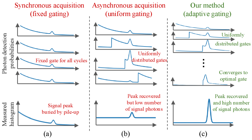
A popular technique for mitigating pile-up is to use gating mechanisms that can selectively activate and deactivate the SPAD at specific time intervals relative to laser pulse emissions. Gating can help prevent the detection of early-arriving background photons, and thus favor the detection of late-arriving signal photons. Prior work has proposed different schemes for selecting gating times. A common such scheme is fixed gating, which uses for all laser pulses the same gating time (Figure 2(a)). If this gating time is close to the time-of-flight corresponding to scene depth, then fixed gating greatly increases the detection probability of signal photons, and thus depth estimation accuracy. Unfortunately, it is not always possible to know or approximate the time-of-flight of true depth ahead of time.
More recently, Gupta et al. [15] proposed a uniform gating scheme, which uniformly distributes gate times for successive laser pulses across the entire depth range (Figure 2(b)). This helps “average-out” the effect of pile-up across all possible depths. Unfortunately, uniform gating does not take into account information about the true scene depth available from either prior knowledge, or from photon detections during previous laser pulses.
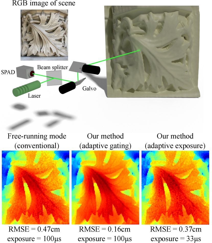
We propose a new gating scheme for SPAD-based LiDAR that we term adaptive gating. Two main building blocks underlie our gating scheme: First, a probabilistic model for the detection times recorded by SPAD-based LiDAR. Second, the classical Thompson sampling algorithm for sequential experimental design. By combining these two components, our proposed adaptive gating scheme is able to select gating sequences that, at any time during LiDAR acquisition, optimally take advantage of depth information available at that time, either from previous photon detections or from some depth prior. As a useful by-product of our framework, we introduce a variant of our adaptive gating scheme that additionally adapts exposure time, as necessary to achieve some target depth accuracy. We build a SPAD-based LiDAR prototype, and perform experiments both indoors, and outdoors under strong sunlight. Our experiments show that, compared to previous gating schemes, our adaptive gating scheme can reduce either depth estimation error or acquisition time (or both) by more than (Figure 1), and can take advantage of prior depth information from spatial regularization or RGB images. To ensure reproducibility and facilitate follow-up research, we provide our code and data on the project website [36].
2 Related work
Post-processing for pile-up compensation. There is extensive prior work on post-processing techniques for compensating the effects of pile-up. Perhaps the best known is Coates’ technique [12], and its generalizations [33, 15, 16, 19, 38, 37]. Coates’ technique uses a probabilistic model for photon arrivals to estimate the true incident scene transient, from which we can estimate depth. Alternatively, Heide et al. [17] use the same probabilistic model to perform maximum likelihood estimation directly for depth. We discuss how these approaches relate to our work in Section 3.
Gating schemes. Gating refers to the process of desynchronizing laser pulse emission and SPAD acquisition, and is commonly used to mitigate the effects of pile-up. The most common gating technique, known as fixed gating, uses a fixed delay between laser pulse emission and the start of SPAD acquisition, suppressing the detection of early-arriving photons. If the gating delay approximately matches the scene depth, fixed gating significantly reduces pile-up; otherwise, fixed gating will either have no significant effect, or may even suppress signal photons if the gating delay is after the scene depth. Gupta et al. [15] introduced a gating technique that uses uniformly-distributed delays spanning the entire depth range of the SPAD. This uniform gating technique helps mitigate pile-up, without requiring approximate knowledge of scene depth. Lastly, Gupta et al. [15] showed that it is possible to achieve uniformly-distributed delays between pulse emission and the start of SPAD acquisition by operating the SPAD without gating, at free-running mode [20, 13, 3, 37, 38]. We discuss fixed gating, uniform gating, and free-running mode in Section 4.
Spatially-adaptive LiDAR. SPAD-based LiDAR typically uses beam steering to raster-scan individual pixel locations. Recent work has introduced several techniques that, instead of performing a full raster scan, adaptively select spatial locations to be scanned, in order to accelerate acquisition [8, 35, 49]. These techniques are complementary to ours: Whereas they adaptively sample spatial scan locations, our technique adaptively samples temporal gates.
Other LiDAR technologies. There are several commercially-available technologies for light detection and ranging (LiDAR), besides SPAD-based LiDAR [39]. A common alternative in autonomous vehicles uses avalanche photodiodes (APDs) [25]. Compared to SPAD-based LiDAR, APD-based LiDAR does not suffer from pile-up, but has reduced sensitivity. Other LiDAR systems use continuous-wave time-of-flight (CWToF) cameras [14, 46, 22]. CWToF-based LiDAR is common in indoor 3D applications [45, 42, 4]. Unlike SPAD-based and APD-based LiDAR, CWToF-based LiDAR is sensitive to global illumination (multi-path interference).
Other SPAD applications. SPADs find use in biophotonics applications [10], including fluorescence-lifetime imaging microscopy [23, 9, 5, 24, 44], super-resolution microscopy [28], time-resolved Raman spectroscopy [28], and time-domain diffuse optical tomography [50, 34]. Other applications include non-line-of-sight imaging [48, 11, 30, 27], and high-dynamic-range imaging [19, 18].
3 Background on SPAD-based LiDAR
We discuss necessary background on 3D imaging with single-photon avalanche diodes (SPADs). We consider single-pixel SPAD-based LiDAR systems with controllable gating. Such a system comprises: a) an ultrafast pulsed laser that can emit short-duration light pulses at a pulse-to-pulse frequency (or repetition rate) ; b) a single-pixel SPAD that can detect individual incident photons; c) gating electronics that can activate the SPAD at some controllable time after pulse emissions; and d) time-correlation electronics that time photon detections relative to pulse emissions. We assume that both the gating and time-correlation electronics have the same temporal resolution . Typical orders of magnitude are a few for pulse duration, hundreds of for , and tens of for . The laser and SPAD are commonly coaxial, and rely on beam steering (e.g., through a galvo or MEMS mirror) to produce 2D depth estimates. Figure 1 shows a schematic of such a setup.
At each scan point, the LiDAR uses time-correlated single photon counting (TCSPC) to estimate depth. This process comprises cycles, where at each cycle a sequence of steps takes place: At the start of the -th cycle, the laser emits a pulse. Gating activates the SPAD at gate time after the start of the cycle. The SPAD remains active until it detects the first incident photon (originating from either the laser pulse or ambient light) at detection time after the start of the cycle. It then enters a dead time, during which it cannot detect any photons. Once the dead time ends, the SPAD remains inactive until the next pulse emission, at which point the next cycle begins. We note that there can be multiple pulse emissions during a single cycle. After cycles, the LiDAR system returns the sequence of detection times , measured using the sequence of gate times . 111Prior works [15, 16, 17, 37, 38] typically study the detected photon histogram, and not the sequence of detection times. As we discuss in the supplement, the two formulations are consistent. We discretize the time between pulse emissions into temporal bins, where the -th bin corresponds to the time interval since pulse emission. Then, the range of gate times is , and the range of detection times is . 222This assumes that the SPAD always detects a photon during a period of after it becomes active. In practice, the SPAD may detect no photon. We ignore this for simplicity, and refer to Gupta et al. [15] for details. We describe a probabilistic model for (Section 3.1), then see how to estimate depth from it (Section 3.2).
3.1 Probabilistic model
Our model closely follows the asynchronous image formation model of Gupta et al. [15]. 333We refer to the supplement for a discussion of the assumptions made by this model (e.g., infinitesimal pulse duration) and their implications. We first consider the incident photon histogram : for each bin , is the number of photons incident on the SPAD during the time interval since the last pulse emission. The subscript indicates that the histogram depends on scene depth, as we explain shortly. We model each as a Poisson random variable,
| (1) |
with rate equal to,
| (2) |
The function is the scene transient [21, 32]. In Equation (2), the ambient flux is the average number of incident background photons (i.e., photons due to ambient light) at the SPAD during time , which we assume to be time-independent. The signal flux is the average number of incident signal photons (i.e., photons due to the laser). and depend on scene reflectivity and distance, and the flux of ambient light (for ) and laser pulses (for ). We refer to their ratio as the signal-to-background ratio . 444Prior works [15, 16] define . We omit , to make SBR indicative of the difficulty in resolving the signal bin from the background bins. is the Kronecker delta, and , where is the scene distance and is the speed of light. We use as a proxy for depth.
We now consider the -th cycle of the LiDAR operation. Given that, the SPAD can only detect the first incident photon after activation, a detection time of means that: i) there were no incident photons during the time bins ; and ii) there was at least one incident photon at time bin . The probability of this event occurring is: 555We use the notational convention that , , are random variables, and , , are specific values for these random variables.
| (3) |
To simplify notation, in the rest of the paper we use:
| (4) |
Using Equation (1), we can rewrite this probability as:
| (5) |
Lastly, we define the detection sequence likelihood:
| (6) |
Given that the detection times are conditionally independent of each other given the gate times, we have
| (7) |
Equations (2), (5), and (7) fully determine the probability of a sequence of detection times , measured using a sequence of gate times , assuming scene depth .
Pile-up. We consider the case where we fix for all cycles ; that is, gating always activates the SPAD at the start of a cycle. Then, Equation (5) becomes
| (8) |
Equations (8) and (2) show that, when the ambient flux is large (e.g., outdoors operation), the probability of detecting a photon at a later time bin is small. This effect, termed pile-up [12, 16], can result in inaccurate depth estimates as scene depth increases. As we discuss in Section 4, carefully selected gate sequences can mitigate pile-up.
3.2 Depth estimation
We now describe how to use the probabilistic model of Section 3.1 to estimate the scene depth from and .
Coates’ depth estimator. Gupta et al. [16, 15] adopt a two-step procedure for estimating depth. First, they form the maximum likelihood (ML) estimate of the scene transient given the detection and gate sequences:
| (9) |
The likelihood function in Equation (9) is analogous to that in Equations (5) and (7), with an important difference: Whereas Equation (5) assumes that the scene transient has the form of Equation (2), the ML problem of Equation (9) makes no such assumption and estimates an arbitrarily-shaped scene transient . Gupta et al. [15] derive a closed-form expression for the solution of Equation (9), which generalizes the Coates’ estimate of the scene transient [12] for arbitrary gate sequences .
Second, they estimate depth as:
| (10) |
This estimate assumes that the true underlying scene transient is well-approximated by the model of Equation (2). We refer to as the Coates’ depth estimator.
MAP depth estimator. If we assume that the scene transient has the form of Equation (2), then Equations (5) and (7) directly connect the detection times and depth , eschewing the scene transient. If we have available some prior probability on depth, we can use Bayes’ rule to compute the depth posterior:
| (11) |
We adopt maximum a-posteriori (MAP) estimation:
| (12) |
When using a uniform prior, the depth posterior and the detection sequence likelihood are equal, and the MAP depth estimator is also the ML depth estimator. We note that Heide et al. [17] proposed a similar MAP estimation approach, using a total variation prior that jointly constrains depth at nearby scan points.
It is worth comparing the MAP and Coates’ depth estimators. First, the two estimators have similar computational complexity. This is unsurprising, as the expressions for the depth posterior of Equation (11) and the Coates’ estimate of Equation (9) are similar, both using the likelihood functions of Equations (5) and (7). A downside of the MAP estimator is that it requires knowing and in Equation (2). In practice, we found it sufficient to estimate the background flux using a small percentage of the total SPAD cycles, and to marginalize the signal flux using a uniform prior.
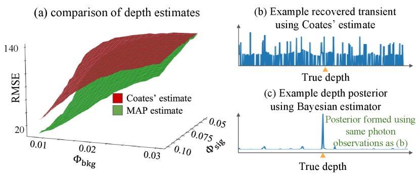
Second, when using a uniform prior, the MAP estimator can provide more accurate estimates than the Coates’ estimator, in situations where the scene transient model of Equation (2) is accurate. To quantify this advantage, we applied both estimators on measurements we simulated for different values of background and signal flux, assuming a uniform gating scheme [15]: As we see in Figure 3, the MAP estimator outperforms the Coates’ estimator, especially when ambient flux is significantly higher than signal flux. By contrast, the Coates’ estimator can be more accurate than the MAP estimator when the scene transient deviates significantly from Equation (2). This can happen due to multiple peaks (e.g., due to transparent or partial occluders) or indirect illumination (e.g., subsurface scattering, interreflections). In the supplement, we show that, when we combine the MAP estimator with our adaptive gating scheme of Section 4, we obtain correct depth estimates even in cases of such model mismatch.
Third, the MAP estimator allows incorporating, through the prior, available side information about depth (e.g., from scans at nearby pixels, or from an RGB image [47]). Before we conclude this section, we mention that the MAP estimator is the Bayesian estimator with respect to the loss [7]:
| (13) |
where
| (14) |
We will use this fact in the next section, as we use the depth posterior and MAP estimator to develop adaptive gating.
4 Adaptive Gating
We now turn our attention to the selection of the gate sequence . As we mentioned in Section 3, we aim to use gating to mitigate pile-up. We briefly review two prior gating schemes, then introduce our adaptive gating.
Fixed gating. A fixed gating scheme uses the same gate for all TCSPC cycles, . So long as this fixed gate is before the scene depth, , it will prevent the detection of early-arriving photons due to ambient light, and thus increase the probability of detection of signal photons. For fixed gating to be effective, should be close, and ideally equal to the true depth , as setting s maximizes the detection probability in Equation (5). Unfortunately, this requires knowing the true depth , or at least a reliable estimate thereof; such an estimate is generally available only after several cycles.
Uniform gating. Gupta et al. [15] introduced a uniform gating scheme, which distributes gates uniformly across the entire depth range. If, for simplicity, we assume that the numbers of cycles and temporal bins are equal, , then uniform gating sets . This maximizes the detection probability of each bin for a few cycles, and “averages out” pile-up effects. Compared to fixed gating, uniform gating does not require an estimate of the true depth . Conversely, uniform gating cannot take advantage of increasing information about as more cycles finish.
Gupta et al. [15] propose using the SPAD in free-running mode without gating—the SPAD becomes active immediately after dead time ends—as an alternative to uniform gating. As they explain, using free-running mode also ensures that all bins have high probability of detection for a few cycles, similar to uniform gating; and provides additional advantages (e.g., maximizes SPAD active time, simplifies hardware). Therefore, we often compare against free-running mode instead of uniform gating.
Desired behavior for adaptive gating. Before formally describing our adaptive gating scheme, we describe at a high-level the desired behavior for such a scheme. Intuitively, an ideal gating scheme should behave as a hybrid between fixed and uniform gating. During the early stages of LiDAR operation (first few cycles) we have little to no information about scene depth—all temporal bins have approximately equal probability of being the true depth. Thus, a hybrid scheme should mimic uniform gating to explore the entire depth range. During the later stages of LiDAR operation (last few cycles), we have rich information about scene depth from the detection times recorded during preceding cycles—only one or few temporal bins have high probability of being the true depth. Thus, a hybrid scheme should mimic (near-fixed) gating, to maximize the detection probability of the few remaining candidate temporal bins. At intermediate stages of LiDAR operation, the hybrid scheme should progressively transition from uniform towards fixed gating, with this progression adapting from cycle to cycle to the information about scene depth available from previously-recorded detection times.
Thompson sampling. To turn the above high-level specification into a formal algorithm, we use two building blocks. First, we use the probabilistic model of Section 3 to quantify the information we have about scene depth at each cycle. At the start of cycle , the LiDAR has recorded detection times using gate times . Then, the depth posterior of Equation (11) represents all the information we have available about scene depth, from both recorded detection times and any prior information ().
Second, we use Thompson sampling [43] to select the gate times . Thompson sampling is a classical algorithm for online experimental design: This is the problem setting of deciding on the fly parameters of a sequence of experiments, using at any given time available information from all experiments up to that time, in a way that maximizes some utility function [41]. Translating this into the context of SPAD-based LiDAR, the sequence of experiments is the TCSPC cycles; at the -th experiment, the parameter to be decided is the gate time . and the available information is the depth posterior ; lastly the utility function is the accuracy of the final depth estimate. Thompson sampling selects each gate by first sampling a depth hypothesis from the depth posterior , and then finding the gate time that maximizes a reward function . Algorithm 1 shows the resulting adaptive gating scheme (blue lines correspond to modifications we describe in Section 5).
Reward function. We motivate our choice of reward function as follows: At cycle , Thompson sampling assumes that the true depth equals the depth hypothesis sampled from the depth posterior. Equivalently, Thompson sampling assumes that the detection time we will measure after cycle concludes is distributed as (Equation (5)). As we aim to infer depth, we should select a gate such that, if we estimated depth from only the next detection , the resulting estimate would be in expectation close to the depth hypothesis we assume to be true. Formally,
| (15) |
In Equation (15), to estimate depth from the expected detection time , we use the same MAP depth estimator of Equation (12) as for the final depth estimate . The MAP depth estimator is optimal with respect to the loss (Equation (13)), thus we use the same loss for the reward function. Selecting the gate requires maximizing the reward function , which we can do analytically.
Proposition 1.
We provide the proof in the supplement. Intuitively, minimizing the expected loss between the estimate and the depth hypothesis is equivalent to maximizing the probability that ; that is, we want to maximize the probability that a photon detection occurs at the same temporal bin as the depth hypothesis. We do this by setting the gate equal to the depth hypothesis, . 666In practice, we set the gate time a few bins before the depth hypothesis , to account for the finite laser pulse width and timing jitter.
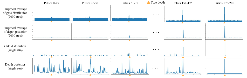
Intuition behind Thompson sampling. Before concluding this section, we provide some intuition about how Thompson sampling works, and why it is suitable for adaptive gating. We can consider adaptive gating with Thompson sampling as a procedure for balancing the exploration-exploitation trade-off. Revisiting the discussion at the start of this section, fixed gating maximizes exploitation, by only gating at one temporal bin (or a small number thereof); conversely, uniform gating maximizes exploration, by gating uniformly across the entire depth range. During the first few cycles, adaptive gating maximizes exploration: as only few measurements are available, the depth posterior is flat, and depth hypotheses (and thus gate times) are sampled approximately uniformly as with uniform gating. As the number of cycles progresses, adaptive gating shifts from exploration to exploitation: additional measurements make the depth posterior concentrated around a few depth values, and gate times are sampled mostly among those. After a sufficiently large number of cycles, adaptive gating maximizes exploitation: the depth posterior peaks at a single depth, and gate times are almost always set to that depth, as in fixed gating. Figure 4 uses simulations to visualize this transition from exploration to exploitation. This behavior matches the one we set out to achieve at the start of this section. Lastly, we mention that Thompson sampling has strong theoretical guarantees for asymptotic optimality [41]; this suggests that our adaptive gating scheme balances the exploration-exploitation trade-off in a way that, asymptotically (given enough cycles), maximizes depth accuracy.
5 Adaptive Exposure
The accuracy of a depth estimate from SPAD measurements depends on three main factors: the exposure time (i.e., number of laser pulses, which also affects the number of cycles ), ambient flux , and signal-to-background ratio SBR. For a fixed exposure time, increasing ambient flux or lowering SBR will result in higher depth estimation uncertainty. Even under conditions of identical ambient flux and SBR, the required exposure time to reach some uncertainty threshold can vary significantly, because of the random nature of photon arrivals and detections.
In a generic scene, different pixels can have very different ambient flux or SBR (e.g., due to cast shadows, varying reflectance, and varying depth). Therefore, using a fixed exposure time will result in either a lot of wasted exposure time on pixels for which shorter exposure times are sufficient, or high estimation uncertainty in pixels that require a longer exposure time. Ideally, we want to adaptively extend or shorten the per-pixel exposure time, depending on how many TCSPC cycles are needed to reach some desired depth estimation uncertainty threshold.
Adaptive gating with adaptive exposure. The adaptive gating scheme of Section 4 lends itself to a modification that also adapts the number of cycles , and thus exposure time. In Algorithm 1, we can terminate the while loop early at a cycle , if the depth posterior becomes concentrated enough that we expect depth estimation to have low error. Formally, we define a termination function as the expected error with respect to the depth posterior:
| (17) | ||||
| (18) |
In Equation (17), we use the same MAP depth estimator as for the final depth estimate , and the loss for which the MAP estimator is optimal (Equation (13)). These choices are analogous to our choices for the definition of the reward function in Equation (15). At the end of each cycle , we check whether the termination function is smaller than some threshold, and terminate acquisition if it is true. In Algorithm 1, we show in blue how we modify our original adaptive gating algorithm to include this adaptive exposure procedure.
6 Experimental Results
We show comparisons using real data from an experimental prototype in the paper, and additional comparisons on real and simulated data in the supplement. Throughout the paper, we use root mean square error (RMSE) as the performance metric, as is common in prior work. In the supplement, we additionally report error metrics; this makes performance improvements more pronounced, as our technique optimizes error (Section 4). Our code and data are available on the project website [36].
Prototype. Our SPAD-based LiDAR prototype comprises a fast-gated SPAD (Micro-photon Devices), a picosecond pulsed laser (NKT Photonics NP100-201-010), a TCSPC module (PicoHarp 300), and a programmable picosecond delayer (Micro-photon Devices). We operated the SPAD in triggered mode (adaptive gating) or free-running mode, with the programmable dead time set to . We set the laser pulse frequency to , with measurements discretized to bins ( resolution). The raster scan resolution is , and acquisition time per scan point is , for a total acquisition time of . We note that, if gate selection happens during dead time—easily achievable with optimized compute hardware—our procedure does not introduce additional acquisition latency.
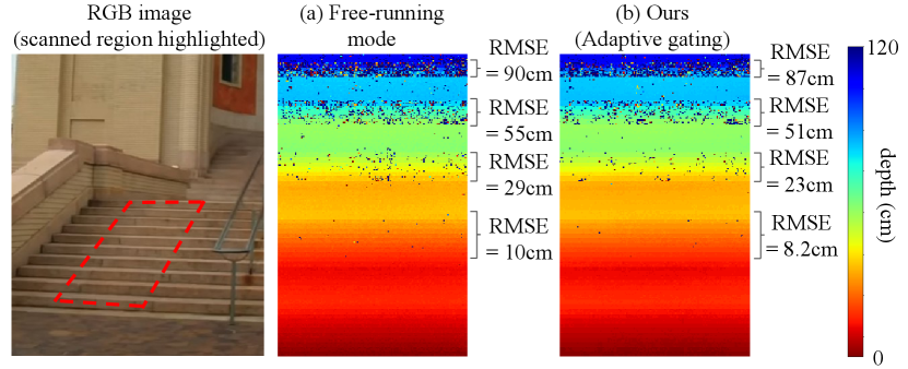
Outdoor scenes. Outdoor experiments (Figures 1 and 5) were under direct sunlight (no shadows or clouds) around noon (11 am to 2 pm in the United States), with an estimated background strength of 0.016 photons per pulse per bin. Figure 1 shows a set of 3D reconstructions for the “Leaf” scene, captured at noon with a clear sky and under direct sunlight. Figures 1(a)-(b) show depth reconstructions using free-running mode and adaptive gating under fixed exposure times: our method reduces RMSE by around . Figure 1(c) shows the depth reconstruction using adaptive gating combined with adaptive exposure. This combination reduces both RMSE and exposure time (by around ) compared to free-running mode. Figure 5 shows depth reconstructions for the “Stairs” scene, captured under the same sunlight conditions. This scene has significant SBR variations, and we observe that adaptive gating outperforms free-running mode in all SBR regimes.
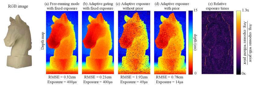
Indoor scenes. Figure 6 shows reconstructions of the “Horse” scene, an indoor scene of a horse bust placed in a light booth. Under fixed exposure time, our method achieves lower RMSE compared to free-running mode. We note that RMSE improvement is less pronounced than in outdoor scenes. As the indoor scene has significantly higher SBR, this suggests that adaptive gating offers a bigger advantage over free-running mode at low SBRs.
We next examine the effectiveness of employing external priors. In Figure 6(c)-(d), we use a “flatness” prior: at each pixel we use a Gaussian prior centered at the depth measured at the previous scanned pixel. Leveraging this simple prior leads to a 70% decrease in exposure time, and a 60% decrease in RMSE compared to adaptive gating without the use of a depth prior. We note, however, that this prior is not effective at pixels corresponding to large depth discontinuities. We can see this in Figure 6(e), which visualizes relative exposure time reduction at different pixels.
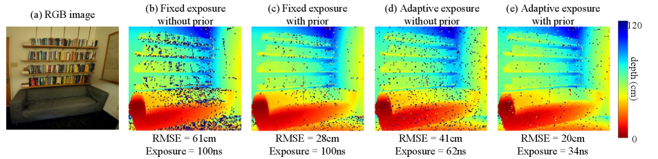
In Figure 7, we use a monocular depth estimation algorithm [47] to obtain depth estimates and uncertainty values from an RGB image of the “Office” scene. We incorporate the monocular prior in our adaptive gating method, and notice a reduction in RMSE for fixed exposure times, and lower total acquisition time using adaptive exposure.
7 Limitations and Conclusion
Active time. As Gupta et al. [15] explain, using free-running mode provides similar advantages as uniform gating, and at the same time maximizes the time during which the SPAD is active—and thus maximizes photon detections. Adaptive gating, likewise, also results in reduced active time compared to free-running mode. However, experimentally we found that, despite the reduced photon detections, our adaptive gating scheme still results in improved depth accuracy for all practical dead time values (see Section 6 and additional experiments evaluating the effect of active and dead time in the supplement).
Hardware considerations. Our adaptive gating scheme requires using a SPAD with a controllable gate that can be reprogrammed from pulse to pulse. We implemented this using the same gated SPAD hardware as Gupta et al. [15] did for their uniform gating scheme. The main additional hardware requirements are electronics that can produce the gate control signals at frequency and resolution. Both gating schemes require considerably more expensive hardware compared to free-running mode operation, which only requires an ungated SPAD. Whether the improved depth accuracy performance justifies the increased hardware cost and complexity is an application-dependent consideration.
Our adaptive exposure scheme additionally requires beam steering hardware that can on the fly change the scan time for any given pixel. Unfortunately, currently this is only possible at the cost of significantly slower overall scanning: Current beam steering solutions for LiDAR must operate in resonant mode to enable scanning rates, which in turn means that the per-pixel scan times are pre-determined by the resonant scan pattern [35]. Thus, using adaptive exposure requires operating beam steering at non-resonant mode. This introduces scanning delays that likely outweigh the gains from reduced per-pixel scan times, resulting in an overall slower scanning rate.
Lastly, recent years have seen the emergence of two-dimensional SPAD arrays [29]. Current prototypes support a shared programmable gate among all pixels. Adaptive gating would require independent per-pixel programmable gates, which can be implemented at increased fabrication cost, and likely decreased sensitive area. As SPAD arrays time-multiplex acquisition across pixels, adaptive exposure does not offer an obvious advantage in this context.
Conclusion. We introduced an adaptive gating scheme for SPAD-based LiDAR that mitigates the effects of pile-up under strong ambient light conditions. Our scheme uses a Thompson sampling procedure to select a gating sequence that takes advantage of information available from previously-measured laser pulses, to maximize depth estimation accuracy. Our scheme can also adaptively adjust exposure time per-pixel, as necessary to achieve a desired expected depth error. We showed that our scheme can reduce both depth error and exposure time by more than compared to previous SPAD-based LiDAR techniques, including when operating outdoors under strong sunlight.
Acknowledgments. We thank Akshat Dave, Ankit Raghuram, and Ashok Veeraraghavan for providing the high-power laser for experiments and invaluable assistance in its use; as well as Matthew O’Toole, David Lindell, and Dorian Chan for help with the SPAD sensor. This work was supported by NSF Expeditions award 1730147, NSF CAREER award 2047341, DARPA REVEAL contract HR0011-16-C-0025, and ONR DURIP award N00014-16-1-2906. Ioannis Gkioulekas is supported by a Sloan Research Fellowship.
References
- [1] The iPhone 12 – LiDAR At Your Fingertips. Forbes (12 November 2020). https://www.forbes.com/sites/sabbirrangwala/2020/11/12/the-iphone-12lidar-at-your-fingertips/. Accessed: 2021-11-17.
- [2] Lidar drives forwards. Nature Photonics, 12:441, 2018.
- [3] Giulia Acconcia, A Cominelli, Massimo Ghioni, and Ivan Rech. Fast fully-integrated front-end circuit to overcome pile-up limits in time-correlated single photon counting with single photon avalanche diodes. Optics express, 26 12:15398–15410, 2018.
- [4] Dean Anderson, Herman Herman, and Alonzo Kelly. Experimental characterization of commercial flash ladar devices. In International Conference of Sensing and Technology, volume 2, pages 17–23. Citeseer, 2005.
- [5] Christopher Barsi, Refael Whyte, Ayush Bhandari, Anshuman Das, Achuta Kadambi, Adrian A Dorrington, and Ramesh Raskar. Multi-frequency reference-free fluorescence lifetime imaging using a time-of-flight camera. In Biomedical Optics, pages BM3A–53. Optical Society of America, 2014.
- [6] Wolfgang Becker. Advanced time-correlated single photon counting applications. Advanced Time-Correlated Single Photon Counting Applications, 2015.
- [7] James O Berger. Statistical decision theory and Bayesian analysis. Springer Science & Business Media, 2013.
- [8] Alexander W Bergman, David B Lindell, and Gordon Wetzstein. Deep adaptive lidar: End-to-end optimization of sampling and depth completion at low sampling rates. In 2020 IEEE International Conference on Computational Photography (ICCP), pages 1–11. IEEE, 2020.
- [9] Ayush Bhandari, Christopher Barsi, and Ramesh Raskar. Blind and reference-free fluorescence lifetime estimation via consumer time-of-flight sensors. Optica, 2(11):965–973, 2015.
- [10] Claudio Bruschini, Harald Homulle, Ivan Michel Antolovic, Samuel Burri, and Edoardo Charbon. Single-photon avalanche diode imagers in biophotonics: review and outlook. Light: Science & Applications, 8(1):1–28, 2019.
- [11] Mauro Buttafava, Jessica Zeman, Alberto Tosi, Kevin W. Eliceiri, and Andreas Velten. Non-line-of-sight imaging using a time-gated single photon avalanche diode. Optics express, 23 16:20997–1011, 2015.
- [12] P. B. Coates. The correction for photon ‘pile-up’ in the measurement of radiative lifetimes. Journal of Physics E: Scientific Instruments, 1:878–879, 1968.
- [13] A Cominelli, Giulia Acconcia, P. Peronio, Massimo Ghioni, and Ivan Rech. High-speed and low-distortion solution for time-correlated single photon counting measurements: A theoretical analysis. The Review of scientific instruments, 88 12:123701, 2017.
- [14] S Burak Gokturk, Hakan Yalcin, and Cyrus Bamji. A time-of-flight depth sensor-system description, issues and solutions. In 2004 conference on computer vision and pattern recognition workshop, pages 35–35. IEEE, 2004.
- [15] Anant Gupta, Atul Ingle, and Mohit Gupta. Asynchronous single-photon 3d imaging. 2019 IEEE/CVF International Conference on Computer Vision (ICCV), pages 7908–7917, 2019.
- [16] Anant Gupta, Atul Ingle, Andreas Velten, and Mohit Gupta. Photon-flooded single-photon 3d cameras. 2019 IEEE/CVF Conference on Computer Vision and Pattern Recognition (CVPR), pages 6763–6772, 2019.
- [17] Felix Heide, Steven Diamond, David B. Lindell, and Gordon Wetzstein. Sub-picosecond photon-efficient 3d imaging using single-photon sensors. Scientific Reports, 8, 2018.
- [18] Atul Ingle, Trevor Seets, Mauro Buttafava, Shantanu Gupta, Alberto Tosi, Mohit Gupta, and Andreas Velten. Passive inter-photon imaging. In Proceedings of the IEEE/CVF Conference on Computer Vision and Pattern Recognition, pages 8585–8595, 2021.
- [19] Atul Ingle, Andreas Velten, and Mohit Gupta. High flux passive imaging with single-photon sensors. 2019 IEEE/CVF Conference on Computer Vision and Pattern Recognition (CVPR), pages 6753–6762, 2019.
- [20] Sebastian Isbaner, Narain Karedla, Daja Ruhlandt, Simon Christoph Stein, Anna M. Chizhik, Ingo Gregor, and Jörg Enderlein. Dead-time correction of fluorescence lifetime measurements and fluorescence lifetime imaging. Optics express, 24 9:9429–45, 2016.
- [21] Adrian Jarabo, Julio Marco, Adolfo Munoz, Raul Buisan, Wojciech Jarosz, and Diego Gutierrez. A framework for transient rendering. ACM Transactions on Graphics (ToG), 33(6):1–10, 2014.
- [22] Achuta Kadambi, Jamie Schiel, and Ramesh Raskar. Macroscopic interferometry: Rethinking depth estimation with frequency-domain time-of-flight. In Proceedings of the IEEE Conference on Computer Vision and Pattern Recognition, pages 893–902, 2016.
- [23] Joseph R Lakowicz, Henryk Szmacinski, Kazimierz Nowaczyk, Klaus W Berndt, and Michael Johnson. Fluorescence lifetime imaging. Analytical biochemistry, 202(2):316–330, 1992.
- [24] Jongho Lee, Jenu Varghese Chacko, Bing Dai, Syed Azer Reza, Abdul Kader Sagar, Kevin W Eliceiri, Andreas Velten, and Mohit Gupta. Coding scheme optimization for fast fluorescence lifetime imaging. ACM Transactions on Graphics (TOG), 38(3):1–16, 2019.
- [25] You Li and Javier Ibanez-Guzman. Lidar for autonomous driving: The principles, challenges, and trends for automotive lidar and perception systems. IEEE Signal Processing Magazine, 37(4):50–61, 2020.
- [26] David B. Lindell, Matthew O’Toole, and Gordon Wetzstein. Single-photon 3d imaging with deep sensor fusion. ACM Transactions on Graphics (TOG), 37:1 – 12, 2018.
- [27] Xiaochun Liu, Ibón Guillén, Marco La Manna, Ji Hyun Nam, Syed Azer Reza, Toan Huu Le, Adrian Jarabo, Diego Gutierrez, and Andreas Velten. Non-line-of-sight imaging using phasor-field virtual wave optics. Nature, 572(7771):620–623, 2019.
- [28] Francesca Madonini and Federica Villa. Single photon avalanche diode arrays for time-resolved raman spectroscopy. Sensors, 21(13):4287, 2021.
- [29] Kazuhiro Morimoto, Andrei Ardelean, Ming-Lo Wu, Arin Can Ulku, Ivan Michel Antolovic, Claudio Bruschini, and Edoardo Charbon. Megapixel time-gated spad image sensor for 2d and 3d imaging applications. Optica, 7(4):346–354, 2020.
- [30] Matthew O’Toole, David B. Lindell, and Gordon Wetzstein. Confocal non-line-of-sight imaging based on the light-cone transform. Nature, 555:338–341, 2018.
- [31] Agata M. Pawlikowska, Abderrahim Halimi, Robert A. Lamb, and Gerald S. Buller. Single-photon three-dimensional imaging at up to 10 kilometers range. Optics express, 25 10:11919–11931, 2017.
- [32] Adithya Pediredla, Ashok Veeraraghavan, and Ioannis Gkioulekas. Ellipsoidal path connections for time-gated rendering. ACM Transactions on Graphics (TOG), 38(4):1–12, 2019.
- [33] Adithya Kumar Pediredla, Aswin C. Sankaranarayanan, Mauro Buttafava, Alberto Tosi, and Ashok Veeraraghavan. Signal processing based pile-up compensation for gated single-photon avalanche diodes. arXiv: Instrumentation and Detectors, 2018.
- [34] Antonio Pifferi, Davide Contini, Alberto Dalla Mora, Andrea Farina, Lorenzo Spinelli, and Alessandro Torricelli. New frontiers in time-domain diffuse optics, a review. Journal of biomedical optics, 21(9):091310, 2016.
- [35] Francesco Pittaluga, Zaid Tasneem, Justin Folden, Brevin Tilmon, Ayan Chakrabarti, and Sanjeev J Koppal. Towards a mems-based adaptive lidar. In 2020 International Conference on 3D Vision (3DV), pages 1216–1226. IEEE, 2020.
- [36] Ryan Po, Adithya Pediredla, and Ioannis Gkioulekas. Project website, 2022. https://imaging.cs.cmu.edu/adaptive_gating.
- [37] Joshua Rapp, Yanting Ma, Robin M. A. Dawson, and Vivek K Goyal. Dead time compensation for high-flux ranging. IEEE Transactions on Signal Processing, 67:3471–3486, 2019.
- [38] Joshua Rapp, Yanting Ma, Robin M. A. Dawson, and Vivek K Goyal. High-flux single-photon lidar. Optica, 8(1):30–39, Jan 2021.
- [39] Joshua Rapp, Julian Tachella, Yoann Altmann, Stephen McLaughlin, and Vivek K Goyal. Advances in single-photon lidar for autonomous vehicles: Working principles, challenges, and recent advances. IEEE Signal Processing Magazine, 37(4):62–71, 2020.
- [40] Alexis Rochas. Single photon avalanche diodes in cmos technology. 2003.
- [41] Daniel Russo, Benjamin Van Roy, Abbas Kazerouni, Ian Osband, and Zheng Wen. A tutorial on Thompson sampling. arXiv preprint arXiv:1707.02038, 2017.
- [42] Ryuichi Tadano, Adithya Kumar Pediredla, and Ashok Veeraraghavan. Depth selective camera: A direct, on-chip, programmable technique for depth selectivity in photography. In Proceedings of the IEEE International Conference on Computer Vision, pages 3595–3603, 2015.
- [43] William R Thompson. On the likelihood that one unknown probability exceeds another in view of the evidence of two samples. Biometrika, 25(3/4):285–294, 1933.
- [44] Erik B van Munster and Theodorus WJ Gadella. Fluorescence lifetime imaging microscopy (flim). Microscopy techniques, pages 143–175, 2005.
- [45] Jarrett Webb and James Ashley. Beginning kinect programming with the microsoft kinect SDK. Apress, 2012.
- [46] Refael Whyte, Lee Streeter, Michael J Cree, and Adrian A Dorrington. Application of lidar techniques to time-of-flight range imaging. Applied optics, 54(33):9654–9664, 2015.
- [47] Zhihao Xia, Patrick Sullivan, and Ayan Chakrabarti. Generating and exploiting probabilistic monocular depth estimates. 2020 IEEE/CVF Conference on Computer Vision and Pattern Recognition (CVPR), pages 62–71, 2020.
- [48] Shumian Xin, Sotiris Nousias, Kiriakos N. Kutulakos, Aswin C. Sankaranarayanan, Srinivasa G. Narasimhan, and Ioannis Gkioulekas. A theory of fermat paths for non-line-of-sight shape reconstruction. 2019 IEEE/CVF Conference on Computer Vision and Pattern Recognition (CVPR), pages 6793–6802, 2019.
- [49] Taiki Yamamoto, Yasutomo Kawanishi, Ichiro Ide, Hiroshi Murase, Fumito Shinmura, and Daisuke Deguchi. Efficient pedestrian scanning by active scan lidar. In 2018 International Workshop on Advanced Image Technology (IWAIT), pages 1–4. IEEE, 2018.
- [50] Yongyi Zhao, Ankit Raghuram, Hyun Kim, Andreas Hielscher, Jacob T Robinson, and Ashok Narayanan Veeraraghavan. High resolution, deep imaging using confocal time-of-flight diffuse optical tomography. IEEE Transactions on Pattern Analysis and Machine Intelligence, 2021.