Adaptive Identification with Guaranteed Performance Under Saturated-Observation and Non-Persistent Excitation

Lantian Zhang and Lei Guo \IEEEmembershipFellow, IEEE This work was supported by the National Natural Science Foundation of China under Grant No. 12288201.Lantian Zhang and Lei Guo are with the Key Laboratory of Systems and Control, Academy of Mathematics and Systems Science, Chinese Academy of Sciences, Beijing 100190, China, and also with the School of Mathematical Science, University of Chinese Academy of Sciences, Beijing 100049, China. (e-mails: zhanglantian@amss.ac.cn, Lguo@amss.ac.cn).

Abstract

This paper investigates adaptive identification and prediction problems for stochastic dynamical systems with saturated output observations, which arise from various fields in engineering and social systems, but up to now still lack comprehensive theoretical studies including guarantees for the estimation performance needed in practical applications. With this impetus, the paper has made the following main contributions: (i) To introduce an adaptive two-step quasi-Newton algorithm to improve the performance of the identification, which is applicable to a typical class of nonlinear stochastic systems with outputs observed under possibly varying saturation. (ii) To establish the global convergence of both the parameter estimators and adaptive predictors and to prove the asymptotic normality, under the weakest possible non-persistent excitation condition, which can be applied to stochastic feedback systems with general non-stationary and correlated system signals or data. (iii) To establish useful probabilistic estimation error bounds for any given finite length of data, using either martingale inequalities or Monte Carlo experiments. A numerical example is also provided to illustrate the performance of the proposed identification algorithm.

{IEEEkeywords}

Asymptotic normality, convergence, non-PE condition, stochastic systems, saturated observations.

1 Introduction

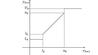
Identifying the input-output relationship and predicting the future behavior of dynamical systems based on observation data are fundamental problems in various fields including control systems, signal processes, machine learning, etc. This paper considers identification and prediction problems for stochastic dynamical systems with saturated output observation data. Here, by saturated output observations, we mean that the observations for the output are produced through the following mechanism: at each time, the noise-corrupted output can be observed precisely only when its value lies in a certain range, however, when the output value exceeds this range, its observation becomes saturated, leading to imprecise information. The relationship between the system output and its observation is illustrated in Fig.1, where $v_{k+1}$ and $y_{k+1}$ represent the system output and its observation respectively, the interval $[l_{k},u_{k}]$ is the precise observation range, when the system output exceeds this range, the only possible observation is a constant, either $L_{k}$ or $U_{k}$ . Note that if we take $L_{k}=l_{k}=0,\;u_{k}=U_{k}=\infty$ , then the saturation function will become the ReLu function widely used in machine learning; and if we take $L_{k}=l_{k}=u_{k}=0,\;U_{k}=1$ , the saturation function will turn to be a binary-valued function widely used in classification problems([mc1943], [gs1990]).

Refer to caption — Figure 1: Saturated output observations.

Saturated output observations in stochastic dynamical systems exist widely in various fields including engineering ([sj2004][hf2009]), economics ([tj1958]-[cm2013]), and social systems[judical]. We only mention several examples in three different application areas. The first example is from control engineering ([sj2004]), where $y_{k}$ represents the sensor observation of the system output, which can be considered as a saturated output observation since it becomes saturated if the output is too large to exceed the observation range of the available sensors. The second example is from economics ([tj1958]), where $v_{k}$ is interpreted as an index of the consumer’s intensity of desire to purchase a durable, $y_{k}$ is the true purchase which can be regarded as a saturated observation, since the intensity $v_{k}$ can be observed only if it exceeds a certain threshold where the true purchase takes place; The third example is from sentencing ([judical]), where $y_{k}$ is the pronounced penalty and can also be regarded as a saturated observation since it is constrained within the statutory range of penalty according to the related basic criminal facts.

Since the emergence of saturation changes the structure of the original systems and may degrade system performance, providing a theoretical analysis for the performance guarantee of the identification algorithm is one of the most important issues addressed in this paper. Compared with the unsaturated case of observations, the key challenge of the current saturated case is the inherent nonlinearity in the observations of the underlying stochastic dynamical systems. In the past several decades, various identification methods with saturated observations have been studied intensively with both asymptotic and non-asymptotic results, on which we give a brief review separately in the following:

First, most of the existing theoretical results are asymptotic in nature, where the number of observations needs to increase unboundedly or at least to be sufficiently large. For example, the least absolute deviation methods were considered in [PJ1984], and the strong consistency and asymptotic normality of the estimators were proven for independent signals satisfying the usual persistent excitation (PE) condition where the condition number of the information matrix is bounded. Besides, the maximum likelihood (ML) method was considered in [ly1992], where consistency and asymptotic efficiency were established for independent or non-random signals satisfying a stronger PE condition. Moreover, a two-stage procedure based on ML was proposed in [hj1976] to deal with two coupled models with saturated observations. Furthermore, the empirical measure approach was employed in [ZG2003]-[YG2007], where strong consistency and asymptotic efficiency were established under periodic signals with binary-valued observations. Such observations were also considered in [GZ2013], where a strongly consistent recursive projection algorithm was given under a condition stronger than the usual PE condition.

Second, there are also a number of non-asymptotic estimation results in the literature. Despite the importance of the asymptotic estimation results as mentioned above, non-asymptotic results appear to be more practical, because one usually only has a finite number of data available for identification in practice. However, obtaining non-asymptotic identification results, which are usually given under high probability, is quite challenging especially when the structure comes to nonlinear. Most of the existing results are established under assumptions that the system data are independently and identically distributed (i.i.d), e.g., the analysis of the stochastic gradient descent methods in [kv2019],[dc2021]. For the dependent data case, an online Newton method was proposed in [po2021], where a probabilistic error bound was given for linear stochastic dynamical systems where the usual PE condition is satisfied.

In summary, almost all of the existing identification results for stochastic dynamical systems with saturated observations need at least the usual PE condition on the system data, and actually, most need i.i.d assumptions. Though these idealized conditions are convenient for theoretical investigation, they are hardly satisfied or verified for general stochastic dynamical systems with feedback signals (see, e.g. [1412020]). This inevitably brings challenges for establishing an identification theory on either asymptotic or non-asymptotic results with saturated observations under more general (non-PE) signal conditions.

Fortunately, there is a great deal of research on adaptive identification for linear or nonlinear stochastic dynamical systems with uncensored or unsaturated observations in the area of adaptive control, where the system data used can include those generated from stochastic feedback control systems. By adaptive identification, we mean that the identification algorithm is constructed recursively, where the parameter estimates are updated online based on both the current estimate and the new observation, and thus the iteration instance depends on the time of the data observed. In comparison with offline algorithms such as those widely used in statistics and machine learning where the iteration instance is the number of search steps in numerical optimization ([yy2015],[sm2018]), the adaptive algorithm has at least two advantages: one is that the algorithm can be updated conveniently when new data come in without restoring the old data, and another is that general non-stationary and correlated data can be handled conveniently due to the structure of the adaptive algorithm. In fact, extensive investigations have been conducted in adaptive identification in the area of control systems for the design of adaptive control laws, where the system data are generated from feedback systems that are far from stationary and hard to be analyzed [g1995]. Many adaptive identification methods have been introduced in the existing literature where the convergence has also been analyzed under certain non-PE conditions (see e.g. [cg1991]-[lw1982]). Among these methods, we mention that Shadab et al. [ss2023] considered the first-order gradient estimator for linear regression models with some finite-time parameter estimation techniques, where the PE condition is replaced with a condition enforced to the determinant of an extended regressor matrix. Ljung [Lj1977] established a convergence theory via the celebrated ordinary differential equation (ODE) method which can be applied to a wide class of adaptive algorithms, where the conditions for regressors are replaced by some stability conditions for the corresponding ODE. Lai and Wei [lw1982] considered the classical least squares algorithm for linear stochastic regression models, and established successfully the strong consistency under the weakest possible non-PE condition. Of course, these results are established for the traditional non-saturated observation case.

The first paper that establishes the strong consistency of estimators for stochastic regression models under general non-PE conditions for a special class of saturated observations (binary-valued observations) appears to be [ZZ2022], where a single-step adaptive quasi-Newton-type algorithm was proposed and analyzed. The non-PE condition used in [ZZ2022] is similar to the weakest possible signal condition for a stochastic linear regression model with uncensored observations (see [lw1982]), which can be applied to non-stationary stochastic dynamical systems with feedback control. However, there are still some unresolved fundamental problems, for instance, a) How should a globally convergent estimation algorithm be designed for stochastic systems under general saturated observations and non-PE conditions? b) What is the asymptotic distribution of the estimation error under non-PE conditions? c) How to get a useful and computable probabilistic estimation error bound under non-PE conditions when the length of data is finite?

The main purpose of this paper is to solve these problems by introducing an adaptive two-step quasi-Newton-type identification algorithm, refining the stochastic Lyapunov function approach, and applying some martingale inequalities and convergence theorems. Besides, the Monte Carlo method is also found quite useful in computing the estimation error bound. The key feature of the current adaptive two-step quasi-Newton (TSQN) identification algorithm compared to the adaptive single-step quasi-Newton method is that the TSQN algorithm has improved performance under non-PE conditions. The main reasons behind this fact are as follows: (i) The scalar adaptation gain of the single-step quasi-Newton method is constructed by using only the fixed given a priori information about the parameter set, whereas the scalar adaptation gain of the current TSQN algorithm is designed by using the online information to have it improved adaptively. (ii) A regularization factor is also introduced in the TSQN algorithm, which can be taken as a “noise variance” estimate to improve the adaptation algorithm further. To be specific, the main contributions of this paper can be summarized as follows:

•

A new two-step quasi-Newton-type adaptive identification algorithm is proposed for stochastic dynamical systems with saturated observations. The first step is to produce consistent parameter estimates based on the available “worst case” information, which is then used to construct the adaptation gains in the second step for improving the performance of the adaptive identification.
•

Asymptotic results on the proposed new identification algorithm, including strong consistency and asymptotic normality, are established for stochastic dynamical systems with saturated observations under quite general non-PE conditions. The optimality of adaptive prediction or regrets is also established without resorting to any excitation conditions. This paper appears to be the first for adapted identification of stochastic systems with guaranteed performance under both saturated observations and general non-PE conditions.
•

Non-asymptotic error bounds for both parameter estimation and output prediction are also provided, when only a finite length of data is available, for stochastic dynamical systems with saturated observations and no PE conditions. Such bounds can be applied to sentencing computation problems based on practical judicial data [judical].

The remainder of this paper is organized as follows. Section 2 gives the problem formulation; The main results are stated in Section LABEL:ss3; Section LABEL:ss4 presents the proofs of the main results. A numerical example is provided in Section LABEL:ss5. Finally, we conclude the paper with some remarks in Section LABEL:ss6.

2 Problem Formulation

Let us consider the following piecewise linear regression model:

y_{k+1}=S_{k}(\phi_{k}^{\top}\theta+e_{k+1}),\;\;k=0,1,\cdots,

(1)

where $\theta\in\mathbb{R}^{m}(m\geq 1)$ is an unknown parameter vector to be estimated; $y_{k+1}\in\mathbb{R}$ , $\phi_{k}\in\mathbb{R}^{m}$ , $e_{k+1}\in\mathbb{R}$ represent the system output observation, stochastic regressor, and random noise at time $k$ , respectively. Besides, $S_{k}(\cdot):\mathbb{R}\rightarrow\mathbb{R}$ is a non-decreasing time-varying saturation function defined as follows:

S_{k}(x)=\left\{\begin{array}[]{rcl}&L_{k}&{x<l_{k}}\\ &x&{l_{k}\leq x\leq u_{k}}\\ &U_{k}&{x>u_{k}}\end{array}\right.,\;\;\;k=0,1,\cdots,

(2)

where $[l_{k},u_{k}]$ is the given precise observable range, $L_{k}$ and $U_{k}$ are the only observations when the output value exceeds this range.

2.1 Notations and Assumptions

Notations. By $\|\cdot\|$ , we denote the Euclidean norm of vectors or matrices. The spectrum of a matrix $M$ is denoted by $\left\{\lambda_{i}\left\{M\right\}\right\}$ , where the maximum and minimum eigenvalues are denoted by $\lambda_{max}\left\{M\right\}$ and $\lambda_{min}\left\{M\right\}$ respectively. Besides, let $tr(M)$ denote the trace of the matrix $M$ , and by $|M|$ we mean the determinant of the matrix $M$ . Moreover, $\left\{\mathcal{F}_{k},k\geq 0\right\}$ is the sequence of $\sigma-$ algebra together with that of conditional mathematical expectation operator $\mathbb{E}[\cdot\mid\mathcal{F}_{k}]$ , in the sequel we may employ the abbreviation $\mathbb{E}_{k}\left[\cdot\right]$ to $\mathbb{E}\left[\cdot\mid\mathcal{F}_{k}\right]$ . Furthermore, a random variable $X$ belongs to $\mathcal{L}_{2}$ if $\mathbb{E}\|X\|^{2}<\infty,$ and a random sequence $\{X_{k},k\geq 0\}$ is called $\mathcal{L}_{2}$ sequence if $X_{k}$ belongs to $\mathcal{L}_{2}$ for all $k\geq 0$ .

We need the following basic assumptions:

Assumption 1

The stochastic regressor $\{\phi_{k},\mathcal{F}_{k}\}$ is a bounded and adapted sequence, where $\left\{\mathcal{F}_{k},k\geq 0\right\}$ is a non-decreasing sequence of $\sigma-$ algebras. Besides, the true parameter $\theta$ is an interior point of a known convex compact set $D\subseteq\mathbb{R}^{m}$ .

By Assumption 1, we can find an almost surely bounded sequence $\{M_{k},k\geq 0\}$ such that

\sup\limits_{x\in D}|\phi_{k}^{\top}x|\leq M_{k},\;\;a.s.

(3)

Assumption 2

The thresholds $\left\{l_{k},\mathcal{F}_{k}\right\}$ , $\left\{u_{k},\mathcal{F}_{k}\right\}$ , $\left\{L_{k},\mathcal{F}_{k}\right\}$ and $\left\{U_{k},\mathcal{F}_{k}\right\}$ are known adapted stochastic sequences, satisfying for any $k\geq 0$ ,

l_{k}-c\leq L_{k}\leq l_{k}\leq u_{k}\leq U_{k}\leq u_{k}+c,\;\;\;a.s.,

(4)

where $c$ is a $\mathcal{L}_{2}$ non-negative random variable, and

\sup_{k\geq 0}l_{k}<\infty,\;\;\inf_{k\geq 0}u_{k}>-\infty,\;\;\;a.s.

(5)

Remark 1

We note that the inequalities $L_{k}\leq l_{k}\leq u_{k}\leq U_{k}$ are determined by the non-decreasing nature of the saturation function used to characterize the saturated output observations as illustrated in Fig. 1, and that Assumption 2 will be automatically satisfied if $\{L_{k}\}$ and $\{U_{k}\}$ are bounded stochastic sequences. The conditions $(\ref{5})$ and $(\ref{6})$ are general assumptions that are used to guarantee the boundedness of the variances of the output prediction errors in the paper.

Assumption 3

The noise $\{e_{k},\mathcal{F}_{k}\}$ is an $\mathcal{L}_{2}$ martingale difference sequence and there exists a constant $\eta>0$ , such that

\inf\limits_{k\geq 0}\mathbb{E}_{k}\left[|e_{k+1}|^{2}\right]>0,\;\;\sup_{k\geq 0}\mathbb{E}_{k}\left[|e_{k+1}|^{2+\eta}\right]<\infty,\;a.s.

(6)

Besides, the conditional expectation function $G_{k}(x)$ , defined by $G_{k}(x)=\mathbb{E}_{k}\left[S_{k}(x+e_{k+1})\right]$ , is known and differentiable with derivative denoted by $G^{\prime}_{k}(\cdot)$ . Further, there exist a random variable $M>\sup\limits_{k\geq 0}M_{k}$ such that

0<\inf_{|x|\leq M,k\geq 0}G^{\prime}_{k}(x)\leq\sup_{|x|\leq M,k\geq 0}G^{\prime}_{k}(x)<\infty,\;\;a.s.

(7)

|G^{\prime}_{k}(x)-G^{\prime}_{k}(y)|\leq\rho|x-y|,\;a.s.,\;\;\;\forall|x|,|y|\leq M,

(8)

where $\rho$ is a non-negative variable, $M_{k}$ is defined in $(\ref{Mk})$ .

Remark 2

It is worth to mention that under condition $(\ref{e})$ , the function $G_{k}(\cdot)$ in Assumption 3 is well-defined for any $k\geq 0$ , and can be calculated given the conditional probability distribution of the noise $e_{k+1}$ . In Appendix LABEL:i, we have provided three typical examples to illustrate how to concretely calculate the function $G_{k}(\cdot)$ , which includes the classical linear stochastic regression models, models with binary-valued sensors, and censored regression models. Moreover, Assumption 3 can be easily verified if the noise $\{e_{k+1},\;k\geq 0\}$ is i.i.d Gaussian and if $\inf\limits_{k\geq 0}(U_{k}-L_{k})>0,\;a.s$ . Besides, when $l_{k}=-\infty$ and $u_{k}=\infty$ , the system $(\ref{eq1})$ - $(\ref{eq2})$ will degenerate to linear stochastic regression models, and Assumption 3 will degenerate to the standard noise assumption for the strong consistency of the classical least squares ([lw1982]) since $G_{k}(x)\equiv x$ .

For simplicity of notation, denote

\inf_{|x|\leq M_{k}}G^{\prime}_{k}(x)=\underline{g}_{k},\;\;\sup_{|x|\leq M_{k}}G^{\prime}_{k}(x)=\overline{g}_{k}.

(9)

Under Assumption 3, $\{\overline{g}_{k},k\geq 0\}$ and $\{\underline{g}_{k},k\geq 0\}$ have upper bound and positive lower bound respectively, i.e.

\inf\limits_{k\geq 0}\underline{g}_{k}>0,\;\;\;\;\;\;\sup\limits_{k\geq 0}\overline{g}_{k}<\infty,\;\;\;\;a.s.

(10)

2.2 Algorithm

Because of its “optimality” and fast convergence rate, the classical LS algorithm is one of the most basic and widely used ones in the adaptive estimation and adaptive control of linear stochastic systems. Inspired by the analysis of the LS recursive algorithm, we have introduced an adaptive quasi-Newton-type algorithm to estimate the parameters in linear stochastic regression models with binary-valued observations in [ZZ2022]. However, we find that a direct extension of the quasi-Newton algorithm introduced in [ZZ2022] from binary-valued observation to saturated observation does not give satisfactory performance, which motivates us to introduce a two-step quasi-Newton-type identification algorithm as described shortly.

At first, we introduce a suitable projection operator, to ensure the boundedness of the estimates while keeping other nice properties. For the linear space $\mathbb{R}^{m}$ , we define a norm $\|\cdot\|_{Q}$ associated with a positive definite matrix $Q$ as $\|x\|_{Q}^{2}=x^{\top}Qx$ . A projection operator based on $\|\cdot\|_{Q}$ is defined as follows:

Definition 1

For the convex compact set $D$ defined in Assumption 1, the projection operator $\Pi_{Q}(x)(\cdot)$ is defined as

\Pi_{Q}(x)=\mathop{\arg\min}_{y\in D}\|x-y\|_{Q},\quad\forall x\in\mathbb{R}^{m}.

(11)

We then introduce our new adaptive two-step quasi-Newton (TSQN) identification algorithm, where the gain matrix is constructed by using the gradient information of the quadratic loss function.

Algorithm 1 Adaptive Two-Step Quasi-Newton (TSQN) Algorithm

Step 1. Recursively calculate the preliminary estimate $\bar{\theta}_{k+1}$ for $k\geq 0$ :

$\displaystyle\bar{\theta}_{k+1}$	$\displaystyle=\Pi_{\bar{P}_{k+1}^{-1}}\{\bar{\theta}_{k}+\bar{a}_{k}\bar{\beta}_{k}\bar{P}_{k}\phi_{k}[y_{k+1}-G_{k}(\phi_{k}^{\top}\bar{\theta}_{k})]\},$	(12)
$\displaystyle\bar{P}_{k+1}$	$\displaystyle=\bar{P}_{k}-\bar{a}_{k}\bar{\beta}_{k}^{2}\bar{P}_{k}\phi_{k}\phi_{k}^{\top}\bar{P}_{k},$
$\displaystyle\bar{\beta}_{k}$	$\displaystyle=\min\left(\underline{g}_{k},\frac{1}{1+2\overline{g}_{k}\phi_{k}^{\top}\bar{P}_{k}\phi_{k}}\right),$
$\displaystyle\bar{a}_{k}$	$\displaystyle=\frac{1}{1+\bar{\beta}_{k}^{2}\phi_{k}^{\top}\bar{P}_{k}\phi_{k}},$

where $\underline{g}_{k}$ and $\overline{g}_{k}$ are defined as in $(\ref{g})$ , $\Pi_{\bar{P}_{k+1}^{-1}}$ is the projection operator defined as in Definition 1, $G_{k}(\cdot)$ is defined in Assumption 3, the initial values $\bar{\theta}_{0}$ and $\bar{P}_{0}$ can be chosen arbitrarily in $D$ and with $\bar{P}_{0}>0$ , respectively.

Step 2. Recursively define the accelerated estimate $\hat{\theta}_{k+1}$ based on $\bar{\theta}_{k+1}$ for $k\geq 0$ :

$\displaystyle\hat{\theta}_{k+1}=$	$\displaystyle\Pi_{P_{k+1}^{-1}}\{\hat{\theta}_{k}+a_{k}\beta_{k}P_{k}\phi_{k}[y_{k+1}-G_{k}(\phi_{k}^{\top}\hat{\theta}_{k})]\},$	(13)
$\displaystyle P_{k+1}=$	$\displaystyle P_{k}-a_{k}\beta_{k}^{2}P_{k}\phi_{k}\phi_{k}^{\top}P_{k},$
$\displaystyle\beta_{k}=$	$\displaystyle\frac{G_{k}(\phi_{k}^{\top}\overline{\theta}_{k})-G_{k}(\phi_{k}^{\top}\hat{\theta}_{k})}{\phi_{k}^{\top}\overline{\theta}_{k}-\phi_{k}^{\top}\hat{\theta}_{k}}I_{\{\phi_{k}^{\top}\hat{\theta}_{k}-\phi_{k}^{\top}\overline{\theta}_{k}\not=0\}}$
	$\displaystyle+G^{\prime}_{k}(\phi_{k}^{\top}\hat{\theta}_{k})I_{\{\phi_{k}^{\top}\hat{\theta}_{k}-\phi_{k}^{\top}\overline{\theta}_{k}=0\}},$
$\displaystyle a_{k}=$	$\displaystyle\frac{1}{\mu_{k}+\beta_{k}^{2}\phi_{k}^{\top}P_{k}\phi_{k}},$

where $\{\mu_{k}\}$ can be any positive random process adapted to $\{\mathcal{F}_{k}\}$ with $0<\inf\limits_{k\geq 0}\mu_{k}\leq\sup\limits_{k\geq 0}\mu_{k}<\infty$ , the initial values $\hat{\theta}_{0}$ and $P_{0}$ can be chosen arbitrarily in $D$ and with $P_{0}>0$ , respectively.