suppSupplementary references
Adaptive Importance Sampling for Finite-Sum Optimization and Sampling with Decreasing Step-Sizes
Abstract
Reducing the variance of the gradient estimator is known to improve the convergence rate of stochastic gradient-based optimization and sampling algorithms. One way of achieving variance reduction is to design importance sampling strategies. Recently, the problem of designing such schemes was formulated as an online learning problem with bandit feedback, and algorithms with sub-linear static regret were designed. In this work, we build on this framework and propose Avare, a simple and efficient algorithm for adaptive importance sampling for finite-sum optimization and sampling with decreasing step-sizes. Under standard technical conditions, we show that Avare achieves and dynamic regret for SGD and SGLD respectively when run with step sizes. We achieve this dynamic regret bound by leveraging our knowledge of the dynamics defined by the algorithm, and combining ideas from online learning and variance-reduced stochastic optimization. We validate empirically the performance of our algorithm and identify settings in which it leads to significant improvements.
1 Introduction
Functions of the form:
| (1) |
are prevalent in modern machine learning and statistics. Important examples include the empirical risk in the empirical risk minimization framework, 111Up to a normalizing factor of which does not affect the optimization or the log-posterior of an exchangeable Bayesian model. When is large, the preferred methods for solving the resulting optimization or sampling problem usually rely on stochastic estimates of the gradient of , using variants of stochastic gradient descent (SGD) [1] or stochastic gradient Langevin dynamics (SGLD) [2]:
| (2) | ||||
| (3) |
where is a sequence of step-sizes, and the index is sampled uniformly from , making an unbiased estimator of the gradient of . We use to refer to either sequence when we do not wish to distinguish between them. It is well known that the quality of the answers given by these algorithms depends on the (trace of the) variance of the gradient estimator, and considerable efforts have been made to design methods that reduce this variance.
In this paper, we focus on the importance sampling approach to achieving variance reduction. At each iteration, the algorithm samples according to a specified distribution , and estimates the gradient using:
| (4) |
It is immediate to verify that is an unbiased estimator of . By cleverly choosing the distributions , one can achieve significant variance reduction (up to a factor of N) compared to the estimator based on uniform sampling. Unfortunately, computing the variance-minimizing distributions at each iteration requires the knowledge of the Euclidean norm of all the individual gradients at each iteration, making it unpractical [3, 4].
Many methods have been proposed that attempt to construct sequences of distributions that result in efficient estimators [3, 4, 5, 6, 7, 8, 9]. Of particular interest to us, the task of designing such sequences was recently cast as an online learning problem with bandit feedback [10, 11, 12, 13]. In this formulation, one attempts to design algorithms with sub-linear expected static regret, which is defined as:
where denotes the probability simplex in , and is the trace of the covariance matrix of the gradient estimator (4), which is easily shown to be:
| (5) |
Note that the second term cancels in the definition of regret, and we omit it in the rest of our discussion. In this formulation, and to keep the computational load manageable, one has only access to partial feedback in the form of the norm of the gradient, and not to the complete cost function (5). Under the assumption of uniformly bounded gradients, the best result in this category can be found in [12] where an algorithm with static regret is proposed. A more difficult but more natural performance measure that makes the attempt to approximate the optimal distributions explicit is the dynamic regret, defined by:
| (6) |
Guarantees with respect to the expected dynamic regret are more difficult to obtain, and require that the cost functions do not change too rapidly with respect to some reasonable measure of variation. See [14, 15, 16, 17, 18] for examples of such measures and the corresponding regret bounds for general convex cost functions.
In this work, we propose Avare, an algorithm that achieves sub-linear dynamic regret for both SGD and SGLD when the sequence of step-sizes is decreasing. The name Avare is derived from adaptive variance minimization. Specifically, our contributions are as follows:
-
•
We show that Avare achieves and dynamic regret for SGD and SGLD respectively when is .
-
•
We propose a new mini-batch estimator that combines the benefits of sampling without replacement and importance sampling while preserving unbiasedness.
-
•
We validate empirically the performance of our algorithm and identify settings in which it leads to significant improvements.
We would like to point out that while the decreasing step size requirement might seem restrictive, we argue that for SGD and SGLD, it is the right setting to consider for variance reduction. Indeed, it is well known that under suitable technical conditions, both algorithms converge to their respective solutions exponentially fast in the early stages. Variance reduction is primarily useful at later stages when the noise from the stochastic gradient dominates. In the absence of control variates, one is forced to use decreasing step-sizes to achieve convergence. This is precisely the regime we consider.
2 Related work
It is easy to see that the cost functions (5) are convex over the probability simplex. A celebrated algorithm for convex optimization over the simplex is entropic descent [19], an instance of mirror descent [20] where the Bregman divergence is taken to be the relative entropy. A slight modification of this algorithm for online learning is the EXP3 algorithm [21] which mixes the iterates of entropic descent with a uniform distribution to avoid the assignment of null probabilities. See [22, 23, 24] for a more thorough discussion of online learning (also called online convex optimization) in general and variants of this algorithm in particular.
Since we are working over the simplex, the EXP3 algorithm is a natural choice. This is the approach taken in [10] and [11], although strictly speaking neither is able to prove sub-linear static regret bounds. The difficulty comes from the fact that the norm of the gradients of the cost functions (5) explode to infinity on the boundary of the simplex. This is amplified by the use of stochastic gradients which grow as in expectation, making it very difficult to reach regions near the boundary. Algorithms based on entropic descent for dynamic regret problems also exist, including the fixed share algorithm and projected mirror descent [25, 26, 27, 28]. Building on these algorithms, and by artificially making the cost functions strongly-convex to allow the use of decreasing step-sizes, we were only able to show dynamic regret using projected mirror descent for SGD with decreasing step sizes and uniformly bounded gradients.
The approach taken in [12] is qualitatively different and is based on the follow-the-regularized-leader (FTRL) scheme. By solving the successive minimization problems stemming from the FTRL scheme analytically, the authors avoid the above-mentioned issue of exploding gradients. The rest of their analysis relies on constructing an unbiased estimate of the cost functions (5) using only the partial feedback , and probabilistically bounding the deviation of the estimated cost functions from the true cost functions using a martingale concentration inequality. The final result is an algorithm that enjoys an static regret bound.
Our approach is similar to the one taken in [12] in that we work directly with the cost functions and not their gradients to avoid the exploding gradient issue. Beyond this point however, our analysis is substantially different. While we are still working within the online learning framework, our analysis is more closely related to the analysis of variance-reduced stochastic optimization algorithms that are based on control variates. In particular, we study a Lyapunov-like functional and show that it decreases along the trajectory of the dynamics defined by the algorithms. This yields simpler and more concise proofs, and opens the door for a unified analysis.
3 Algorithm
Most of the literature on online convex optimization with dynamic regret relies on the use of the gradients of the cost functions [14, 15, 16, 17, 18]. However, as explained in the previous section, such approaches are not viable for our problem. Unfortunately, the regret guarantees obtained from the FTRL scheme for static regret used in [12] do not directly translate into guarantees for dynamic regret.
We start by presenting the high level ideas that go into the construction of our algorithm. We then present our algorithm in explicit form, and discuss its implementation and computational complexity.
3.1 High level ideas
The simplest update rule one might consider when working with dynamic regret is a natural extension of the follow-the-leader approach:
| (7) |
Intuitively, if the cost functions do not change too quickly, then it is reasonable to expect good performance from this algorithm. In our case however, we do not have access to the full cost function. The traditional way of dealing with this problem is to build unbiased estimates of the cost functions using the bandit feedback, and then bounding the deviation of these unbiased estimates from the true cost functions. While this might work, we consider here a different approach based on constructing surrogate cost functions that are not necessarily unbiased estimates of the true costs.
For each , denote by the last observed gradient of at time , with initialized arbitrarily (to for example). We consider the following surrogate cost for all :
| (8) |
As successive iterates of the algorithm become closer and closer to each other, the squared norm of the s become better and better approximations to the squared norm of the s, thereby making the surrogate costs (8) accurate approximations of the true costs (5). The idea of using previously seen gradients to approximate current gradients is inspired by the celebrated variance-reduced stochastic optimization algorithm SAGA [29].
We are now almost ready to formulate our algorithm. If we try to directly minimize the surrogate cost functions over the entire simplex at each iteration as in (7), we might end up assigning null or close to null probabilities to certain indices. Depending on how far we are in the algorithm, this might or might not be a problem. In the initial stages, this is clearly an issue since this might only be an artifact of the initialization (notably when we initialize the to ), or an accurate representation of the current norm of the gradient, but which might not be representative later on as the algorithm progresses. On the other hand, in the later stages of the algorithm, the cost functions are nearly identical, so that an assignment of near zero probabilities is a reflection of the true optimal probabilities, and is not necessarily problematic.
The above discussion suggests the following algorithm. Define the -restricted probability simplex to be:
| (9) |
And let be a decreasing sequence of positive numbers with . Then we propose the following algorithm:
| (10) |
Our theoretical analysis in Section 4 suggests a specific decay rate for the sequence that depends on the sequence of step-sizes and whether SGD or SGLD is run.
3.2 Explicit form
Equation (10) defines our sequence of distribution , but the question remains whether we can solve the implied optimization problems efficiently. In this section we answer this question in the affirmative, and provide an explicit algorithm for the computation of the sequence .
We state our main result of this section in the following lemma. The proof can be found in appendix A.
Lemma 1.
Let be a non-negative set of numbers where at least one of the s is strictly positive, and let . Let be a permutation that orders in a decreasing order (). Define:
| (11) |
and:
| (12) |
Then a solution of the optimization problem:
| (13) |
is given by:
| (14) |
In the case all are zero, any is a solution.
3.3 Implementation details
The naive way to perform the above computation is to do the following at each iteration:
-
•
Sort in decreasing order.
-
•
Find by traversing in increasing order and finding the first for which the inequality in (11) does not hold.
- •
-
•
Sample from using inverse transform sampling.
This has complexity . In appendix A, we present an algorithm that requires only vectorized operations, sequential (non-vectorized) operations, and memory for small . The algorithm uses three data structures:
-
•
An array storing unsorted.
-
•
An order statistic tree storing the pairs sorted according to .
-
•
An array storing where is the permutation that sorts in the order statistic tree.
The order statistic tree along with the array storing the cumulative sums allows the retrieval of in time. The cumulative sums allow to sample from in time using binary search, and maintaining them is the only operation that requires a vectorized operation. All other operations run in time. See appendix A for the full version of the algorithm and a more complete discussion of its computational complexity.
4 Theory
In this section, we prove a sub-linear dynamic regret guarantee for our proposed algorithm when used with SGD and SGLD with decreasing step-sizes. We present our results in a more general setting, and show that they apply to our cases of interest. We start by stating our assumptions:
Assumption 1.
(Bounded gradients) There exists a such that for all and for all .
Assumption 2.
(Smoothness) There exists an such that for all and for all .
Assumption 3.
(Contraction of the iterates in expectation) There exists constants , and such that for all .
The bounded gradients assumption has been used in all previous related work [10, 11, 12, 13], although it is admittedly quite strong. The smoothness assumption is standard in the study of optimization and sampling algorithms. Note that we chose to state our assumptions using index-independent constants to make the presentation clearer and since this does not affect our derivation of the sequence .
Finally, Assumption 3 should really be derived from more basic assumptions, and is only stated to allow for a unified analysis. Note that in the optimization case this is a very mild assumption since we are generally only interested in convergent sequences, and for any such sequence with reasonably fast convergence this assumption holds. The following proposition shows that Assumption 3 holds for our cases of interest. All the proofs for this section can be found in appendix B.
Proposition 1.
We now state a proposition that relates the optimal function value for the problem (13) over the restricted simplex, with the optimal function value over the whole simplex. Its proof is taken from ([12], Lemma 6):
Proposition 2.
Let be a non-negative set of numbers, and let . Then:
The following lemma gives our first bound on the regret per time step:
Lemma 2.
Proof outline.
Let . Then we have the following decomposition:
The terms (A) and (C) are the penalties we pay for using a surrogate cost function, while (B) is the price we pay for restricting the simplex. Using Assumption 1, proposition 2, and the fact that is contained in the -restricted simplex, each of these terms can be bound to give the result stated. ∎
The expectation in the first term of the above lemma is highly reminiscent of the first term of the Lyapunov function used to study the convergence of SAGA first proposed in [30] and subsequently refined in [31] (with replaced by , the gradient at the minimum). Inspired by this similarity, we prove the following recursion:
The natural thing to do at this stage is to unroll the above recursion, replace in Lemma 2, sum over all time steps, and minimize the obtained regret bound over the choice of the sequence . However, even if we can solve the resulting optimization problem efficiently, the solution will still depend on the constants and and on the initial error due to the initialization of the s, both of which are usually unknown. Here instead, we make an asymptotic argument to find the optimal decay rate of , propose a sequence that satisfies this decay rate, and show that it gives rise to the dynamic regret bounds stated.
Denote by the expectation in the first term of the upper bound in Lemma 2. Suppose we take to be of order . Looking at the recursion in Lemma 3, we see that to control the positive term, we need the negative term to be of order at least , so that cannot be smaller than . The bound of Lemma 2 is therefore of order . The minimum is attained when the exponents are equal so we have:
We are now ready to guess the form of . Matching the positive term in Lemma 3, we consider the following sequence:
| (15) |
For a free parameter satisfying to ensure . With this choice of the sequence , we are now finally ready to state our main result of the paper:
Theorem 1.
Proof outline.
Note that since , we have , so is bounded by a constant independent of . Furthermore, setting makes the theorem hold for all . In practice however, it might be beneficial to set to overcome a bad initialization of the s.
5 A new mini-batch estimator
In most practical applications, one uses a mini-batch of samples to construct the gradient estimator instead of just a single sample. The most basic such estimator is the one formed by sampling a mini-batch of indices uniformly and independently, and taking the sample mean. This gives an unbiased estimator, whose variance decreases as . A simple way to make it more efficient is by sampling the indices uniformly but without replacement. In that case, the variance decreases by an additional factor of . For , the difference is negligible, and the additional cost of sampling without replacement is not justified. However, when using unequal probabilities, this argument no longer holds, and the additional variance reduction obtained from sampling without replacement can be significant even for small .
For our problem, besides the additional variance reduction, sampling without replacement allows a higher rate of replacement of the s, which is directly related to our regret through the factor in front of the second term of Lemma 3, whose proper generalization for mini-batch sampling is , where is the inclusion probability of index . This makes sampling without replacement desirable for our purposes. Unfortunately, unlike in the uniform case, the sample mean generalization of (4) is no longer unbiased. We propose instead the following estimator:
| (19) |
We summarize some of its properties in the following proposition:
Proposition 3.
Let for and . We have:
-
(a)
-
(b)
-
(c)
-
(d)
where all the expectations in (d) are conditional on .
The proposed estimator is therefore unbiased and its variance decreases super-linearly in (by (b) and (d)). Although we were unable to prove a regret bound for this estimator, (c) suggests that it is still reasonable to use our algorithm. To take into account the higher rate of replacement of the s, we propose using the following sequence, which is based on the mini-batch equivalent of Lemma 3 and the inequality [32, 33, 34]:
| (20) |
6 Experiments
In this section, we present results of experiments with our algorithm. We start by validating our theoretical results through a synthetic experiment. We then show that our proposed method outperforms existing methods on real world datasets. Finally, we identify settings in which adaptive importance sampling can lead to significant performance gains for the final optimization algorithm.
In all experiments, we added -regularization to the model’s loss and set the regularization parameter . We ran SGD (2) with decreasing step sizes where is the batch size following [35]. We experimented with 3 different samplers in addition to our proposed sampler: Uniform, Multi-armed bandit Sampler (Mabs) [11], and Variance Reducer Bandit (Vrb) \citesuppDBLP:conf/colt/Borsos0L18. The hyperparameters of both Mabs and Vrb are set to the ones prescribed by the theory in the original papers. For our propsoed sampler Avare, we use the epsilon sequence given by (20) with , , and initialized for all . For each sampler, we ran SGD 10 times and averaged the results. The shaded areas represent a one standard deviation confidence interval.
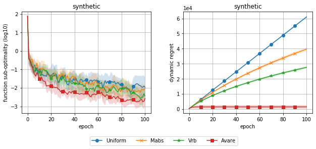
To validate our theoretical findings, we randomly generated a dataset for binary classification with and . We then trained a logistic regression model on the generated data, and used a batch size of 1 to match the setting of our regret bound. The results of this experiment are depicted in figure 1, and show that Avare outperforms the other methods, achieving significantly lower dynamic regret and faster convergence.
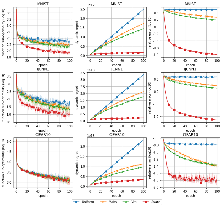
For our second experiment, we tested our algorithm on three real world datasets: MNIST, IJCNN1 [36], and CIFAR10. We used a softmax regression model, and a batch size of 128 sampled with replacement. The results of this experiment can be seen in figure 2. The third column shows the relative error which we define as . In all three cases, Avare achieves significantly smaller dynamic regret, with a relative error quickly decaying to zero. The performance gains in the final optimization algorithm are clear in both MNIST and IJCNN1, but are not noticeable in the case of CIFAR10.
To determine the effectiveness of non-uniform sampling in accelerating the optimization process, previous work [4, 11] has suggested to look at the ratio of the maximum smoothness constant and the average smoothness constant. We show here that this is the wrong measure to look at when using adaptive probabilities. In particular, we argue that the ratio of the variance with uniform sampling at the loss minimizer to the optimal variance at the loss minimizer is much more informative of the performance gains achievable through adaptive importance sampling. For each dataset, these ratios are displayed in Table 1, supporting our claim. We suspect that for large models capable of fitting the data nearly perfectly, our proposed ratio will be large since many of the per-example gradients at the optimum will be zero. We therefore expect our method to be particularly effective in the training of models of this type. We leave such experiments for future work. Finally, in appendix D, we propose an extension of our method to constant step-size SGD, and show that it preserves the performance gains observed when using decreasing step-sizes.
| Dataset | ||
|---|---|---|
| Synthetic | 1.69 | 4.46 |
| MNIST | 3.28 | 5.08 |
| IJCNN1 | 1.12 | 4.83 |
| CIFAR10 | 3.40 | 1.14 |
Broader Impact
Our work develops a new method for variance reduction for stochastic optimization and sampling algorithms. On the optimization side, we expect our method to be very useful in accelerating the training of large scale neural networks, particularly since our method is expected to provide significant performance gains when the model is able to fit the data nearly perfectly. On the sampling side, we expect our method to be useful in accelerating the convergence of MCMC algorithms, opening the door for the use of accurate Bayesian methods at a large scale.
Acknowledgments and Disclosure of Funding
This research was supported by an NSERC discovery grant. We would like to thank the anonymous reviewers for their useful comments and suggestions.
References
- [1] Herbert Robbins and Sutton Monro. A Stochastic Approximation Method. Ann. Math. Statist., 22(3):400–407, 1951.
- [2] Max Welling and Yee Whye Teh. Bayesian Learning via Stochastic Gradient Langevin Dynamics. In Lise Getoor and Tobias Scheffer, editors, Proceedings of the 28th International Conference on Machine Learning, ICML 2011, Bellevue, Washington, USA, June 28 - July 2, 2011, pages 681–688. Omnipress, 2011.
- [3] Deanna Needell, Rachel Ward, and Nathan Srebro. Stochastic Gradient Descent, Weighted Sampling, and the Randomized Kaczmarz algorithm. In Zoubin Ghahramani, Max Welling, Corinna Cortes, Neil D Lawrence, and Kilian Q Weinberger, editors, Advances in Neural Information Processing Systems 27: Annual Conference on Neural Information Processing Systems 2014, December 8-13 2014, Montreal, Quebec, Canada, pages 1017–1025, 2014.
- [4] Peilin Zhao and Tong Zhang. Stochastic Optimization with Importance Sampling for Regularized Loss Minimization. In Francis R Bach and David M Blei, editors, Proceedings of the 32nd International Conference on Machine Learning, ICML 2015, Lille, France, 6-11 July 2015, volume 37 of JMLR Workshop and Conference Proceedings, pages 1–9. JMLR.org, 2015.
- [5] Guillaume Bouchard, Théo Trouillon, Julien Perez, and Adrien Gaidon. Accelerating Stochastic Gradient Descent via Online Learning to Sample. CoRR, abs/1506.0, 2015.
- [6] Sebastian U Stich, Anant Raj, and Martin Jaggi. Safe Adaptive Importance Sampling. In Isabelle Guyon, Ulrike von Luxburg, Samy Bengio, Hanna M Wallach, Rob Fergus, S V N Vishwanathan, and Roman Garnett, editors, Advances in Neural Information Processing Systems 30: Annual Conference on Neural Information Processing Systems 2017, 4-9 December 2017, Long Beach, CA, USA, pages 4381–4391, 2017.
- [7] Angelos Katharopoulos and François Fleuret. Not All Samples Are Created Equal: Deep Learning with Importance Sampling. In Jennifer G Dy and Andreas Krause, editors, Proceedings of the 35th International Conference on Machine Learning, ICML 2018, Stockholmsmässan, Stockholm, Sweden, July 10-15, 2018, volume 80 of Proceedings of Machine Learning Research, pages 2530–2539. PMLR, 2018.
- [8] Tyler B Johnson and Carlos Guestrin. Training Deep Models Faster with Robust, Approximate Importance Sampling. In Samy Bengio, Hanna M Wallach, Hugo Larochelle, Kristen Grauman, Nicolò Cesa-Bianchi, and Roman Garnett, editors, Advances in Neural Information Processing Systems 31: Annual Conference on Neural Information Processing Systems 2018, NeurIPS 2018, 3-8 December 2018, Montréal, Canada, pages 7276–7286, 2018.
- [9] Dominik Csiba and Peter Richtárik. Importance Sampling for Minibatches. J. Mach. Learn. Res., 19:27:1—-27:21, 2018.
- [10] Hongseok Namkoong, Aman Sinha, Steve Yadlowsky, and John C Duchi. Adaptive Sampling Probabilities for Non-Smooth Optimization. In Doina Precup and Yee Whye Teh, editors, Proceedings of the 34th International Conference on Machine Learning, ICML 2017, Sydney, NSW, Australia, 6-11 August 2017, volume 70 of Proceedings of Machine Learning Research, pages 2574–2583. PMLR, 2017.
- [11] Farnood Salehi, L Elisa Celis, and Patrick Thiran. Stochastic Optimization with Bandit Sampling. CoRR, abs/1708.0, 2017.
- [12] Zalan Borsos, Andreas Krause, and Kfir Y Levy. Online Variance Reduction for Stochastic Optimization. In Sébastien Bubeck, Vianney Perchet, and Philippe Rigollet, editors, Conference On Learning Theory, COLT 2018, Stockholm, Sweden, 6-9 July 2018, volume 75 of Proceedings of Machine Learning Research, pages 324–357. PMLR, 2018.
- [13] Zalán Borsos, Sebastian Curi, Kfir Yehuda Levy, and Andreas Krause. Online Variance Reduction with Mixtures. In Kamalika Chaudhuri and Ruslan Salakhutdinov, editors, Proceedings of the 36th International Conference on Machine Learning, ICML 2019, 9-15 June 2019, Long Beach, California, USA, volume 97 of Proceedings of Machine Learning Research, pages 705–714. PMLR, 2019.
- [14] Omar Besbes, Yonatan Gur, and Assaf J Zeevi. Non-Stationary Stochastic Optimization. Oper. Res., 63(5):1227–1244, 2015.
- [15] Xi Chen, Yining Wang, and Yu-Xiang Wang. Non-stationary Stochastic Optimization with Local Spatial and Temporal Changes. CoRR, abs/1708.0, 2017.
- [16] Aryan Mokhtari, Shahin Shahrampour, Ali Jadbabaie, and Alejandro Ribeiro. Online optimization in dynamic environments: Improved regret rates for strongly convex problems. In 55th IEEE Conference on Decision and Control, CDC 2016, Las Vegas, NV, USA, December 12-14, 2016, pages 7195–7201. IEEE, 2016.
- [17] Tianbao Yang, Lijun Zhang, Rong Jin, and Jinfeng Yi. Tracking Slowly Moving Clairvoyant: Optimal Dynamic Regret of Online Learning with True and Noisy Gradient. In Maria-Florina Balcan and Kilian Q Weinberger, editors, Proceedings of the 33nd International Conference on Machine Learning, ICML 2016, New York City, NY, USA, June 19-24, 2016, volume 48 of JMLR Workshop and Conference Proceedings, pages 449–457. JMLR.org, 2016.
- [18] Lijun Zhang, Shiyin Lu, and Zhi-Hua Zhou. Adaptive Online Learning in Dynamic Environments. In Samy Bengio, Hanna M Wallach, Hugo Larochelle, Kristen Grauman, Nicolò Cesa-Bianchi, and Roman Garnett, editors, Advances in Neural Information Processing Systems 31: Annual Conference on Neural Information Processing Systems 2018, NeurIPS 2018, 3-8 December 2018, Montréal, Canada, pages 1330–1340, 2018.
- [19] Amir Beck and Marc Teboulle. Mirror descent and nonlinear projected subgradient methods for convex optimization. Operations Research Letters, 2003.
- [20] A. S. Nemirovsky and D. B. Yudin. Problem Complexity and Method Efficiency in Optimization. The Journal of the Operational Research Society, 1984.
- [21] Peter Auer, Nicolò Cesa-Bianchi, Yoav Freund, and Robert E Schapire. The Nonstochastic Multiarmed Bandit Problem. SIAM J. Comput., 32(1):48–77, 2002.
- [22] Martin Zinkevich. Online Convex Programming and Generalized Infinitesimal Gradient Ascent. In Tom Fawcett and Nina Mishra, editors, Machine Learning, Proceedings of the Twentieth International Conference (ICML 2003), August 21-24, 2003, Washington, DC, USA, pages 928–936. AAAI Press, 2003.
- [23] Shai Shalev-Shwartz. Online Learning and Online Convex Optimization. Foundations and Trends in Machine Learning, 4(2):107–194, 2012.
- [24] Elad Hazan. Introduction to Online Convex Optimization. Found. Trends Optim., 2(3-4):157–325, 2016.
- [25] Mark Herbster and Manfred Warmuth. Tracking the Best Expert. In Armand Prieditis and Stuart Russell, editors, Machine Learning Proceedings 1995, pages 286–294. Morgan Kaufmann, San Francisco (CA), 1995.
- [26] Mark Herbster and Manfred K Warmuth. Tracking the Best Linear Predictor. J. Mach. Learn. Res., 1:281–309, sep 2001.
- [27] Nicolò Cesa-Bianchi, Pierre Gaillard, Gábor Lugosi, and Gilles Stoltz. Mirror Descent Meets Fixed Share (and feels no regret). In Peter L Bartlett, Fernando C N Pereira, Christopher J C Burges, Léon Bottou, and Kilian Q Weinberger, editors, Advances in Neural Information Processing Systems 25: 26th Annual Conference on Neural Information Processing Systems 2012. Proceedings of a meeting held December 3-6, 2012, Lake Tahoe, Nevada, United States, pages 989–997, 2012.
- [28] András György and Csaba Szepesvári. Shifting Regret, Mirror Descent, and Matrices. In Maria-Florina Balcan and Kilian Q Weinberger, editors, Proceedings of the 33nd International Conference on Machine Learning, ICML 2016, New York City, NY, USA, June 19-24, 2016, volume 48 of JMLR Workshop and Conference Proceedings, pages 2943–2951. JMLR.org, 2016.
- [29] Aaron Defazio, Francis R. Bach, and Simon Lacoste-Julien. SAGA: A fast incremental gradient method with support for non-strongly convex composite objectives. CoRR, abs/1407.0202, 2014.
- [30] Thomas Hofmann, Aurélien Lucchi, Simon Lacoste-Julien, and Brian McWilliams. Variance Reduced Stochastic Gradient Descent with Neighbors. In Corinna Cortes, Neil D Lawrence, Daniel D Lee, Masashi Sugiyama, and Roman Garnett, editors, Advances in Neural Information Processing Systems 28: Annual Conference on Neural Information Processing Systems 2015, December 7-12, 2015, Montreal, Quebec, Canada, pages 2305–2313, 2015.
- [31] Aaron Defazio. A Simple Practical Accelerated Method for Finite Sums. In Daniel D Lee, Masashi Sugiyama, Ulrike von Luxburg, Isabelle Guyon, and Roman Garnett, editors, Advances in Neural Information Processing Systems 29: Annual Conference on Neural Information Processing Systems 2016, December 5-10, 2016, Barcelona, Spain, pages 676–684, 2016.
- [32] Yaming Yu. On the inclusion probabilities in some unequal probability sampling plans without replacement. Bernoulli, 18(1):279–289, 2012.
- [33] Hartmut Milbrodt. Comparing inclusion probabilities and drawing probabilities for rejective sampling and successive sampling. Statistics and Probability Letters, 14(3):243–246, 1992.
- [34] Talluri Rao, Samindranath Sengupta, and B Sinha. Some order relations between selection and inclusion probabilities for PPSWOR sampling scheme. Metrika, 38:335–343, 1991.
- [35] Sebastian U. Stich. Unified optimal analysis of the (stochastic) gradient method, 2019.
- [36] Chih-Chung Chang and Chih-Jen Lin. Libsvm: A library for support vector machines. ACM Trans. Intell. Syst. Technol., 2(3), May 2011.
Appendix A Algorithm
A.1 Proof of Lemma 1
See 1
Proof.
Edge case and well-definedness.
If for all , then the objective function is identically over for all , so that any is a solution (we set in the objective). Else there exists an such that , and therefore . Now:
The last inequality is true, so it implies the first, and we have:
Therefore is well defined and is . As a consequence, is also well defined and is , making in turn well-defined.
Optimality proof.
It is easily verified that problem (13) is convex. Its Lagrangian is given by:
and the KKT conditions are:
| (Stationarity) | |||
| (Complementary slackness) | |||
| (Primal feasibility) | |||
| (Dual feasibility) |
By convexity of the problem, the KKT conditions are sufficient conditions for global optimality. To show that our proposed solution is optimal, it therefore suffices to exhibit constants and that together with satisfy these conditions. Let:
Note that the s are well defined since when , , and for all . We claim that the triplet satisfies the KKT conditions.
Stationarity and complementary slackness are immediate from the definitions. The first clause of primal feasibility holds by definition of for . In the other case we have:
where in the third line we used the fact that orders in decreasing order, and in the last line we used the inequality in the definition of . For the second clause of primal feasibility:
Finally, dual feasibility holds by definition of for . In the other case we have:
The first factor is positive by positivity of and non-negativity of the s. For the second factor, we have by the maximality of :
| (21) |
Therefore the second factor is also positive, and dual feasibility holds. ∎
A.2 Implementation and complexity
In this section of the appendix, we provide pseudocode for the implementation of the algorithm and discuss its computational complexity.
A.2.1 Implementation
We assume in algorithm 1 that an order statistic tree (OST) (see, for example, \citesuppDBLP:books/daglib/0023376, chapter 14) can be instantiated and that the ordering in the tree is such that the key of the left child of a node is greater than or equal to that of the node itself. Furthermore, we assume that the method returns the position of in the order determined by an inorder traversal of the tree. Finally, the method returns the value of the -largest key in the tree.
The algorithm works as follows. At initialization, three data structures are initialized: an arrray holding the gradient norms according to the original indices, an order statistic tree holding the gradient norms as keys and the original indices as values, and an array holding the cumulative sums of the gradient norms, where the sums are accumulated in the (decreasing) order that sorts the gradients norms in .
The method allows to sample from the optimal distribution on . It uses the method to find by searching the tree and using the maximality property of . Once is determined, can be calculated. Using the fact that the cumulative sums are proportional to the CDF of the distribution, the algorithm then samples an index using inverse-transform sampling. The sampled index is then transformed back to an index in the original order using the method of the tree .
Finally, the method replaces the gradient norm of a given index by a new one. It calls the methods and which perform the deletion and insertion while maintaining the tree and array .
A.2.2 Complexity
First, let us analyze the cost of running the method. For the array , we only use random access and assignment, which are both . For the tree , we use the methods , , and , all of which are . Finally, for the array we add and subtract from a sub-array, which takes time, although this operation is vectorized and very fast in practice.
Let us now look at the cost of running . The method is recursive, but will only be called at most as many times as the height of the tree, which is . Now for each call of , both the and methods of the tree require time. The rest of the method only requires operations. The total cost of the method is therefore . For the rest of the method, the operations that dominate the cost are the method of the tree , which takes time, and the binary search in the else branch, which also runs in time. Consequently, the total cost of the sample method is .
The total per iteration cost of using the proposed sampler is therefore vectorized operations, and sequential (non-vectorized) operations. The total memory cost is .
Appendix B Theory
B.1 Proof of proposition 1
See 1
Proof.
Conditioning on the knowledge of we have for SGD:
and for SGLD we have:
where in the first line we used the triangle inequality, in the second we used Jensen’s inequality, and in the last we used the fact that is decreasing. Replacing with the value of we obtain the result. ∎
B.2 Proof of proposition 2
Proof.
By Lemma 1 we have:
where in the third line we used inequality (21) from the proof of Lemma 1. Now for the case we have , so the second term in the first line is zero and the inequality becomes an equality:
| (22) |
The difference is therefore bounded by:
where in the last line we used the inequality for which gives the restriction . ∎
B.3 Proof of Lemma 2
See 2
Proof.
Let and . We have the following decomposition:
We bound each term separately:
| (A) | |||
where in the third line we used Assumption 1 and the reverse triangle inequality, and in the last line we used the fact that . Since , we can apply proposition 2 on (B) to obtain:
| (B) |
where the second inequality uses Assumption 1. Finally, using the optimal function values (22) we have for (C):
| (C) | |||
where we again used Assumption 1 and the reverse triangle inequality in the third line. the last inequality follows from the fact that . Combining the three bounds gives the result. ∎
B.4 Proof of Lemma 3
See 3
B.5 Lemma 4
Before proving Theorem 1, we first state and prove the following solution of the recursion of Lemma 3 assuming the sequence is given by (15).
Lemma 4.
Proof.
A simple inequality.
Suppose , then:
otherwise, we have:
where the last inequality follows from the fact that and . We conclude that:
Induction proof.
Let , and let . For the statement holds since:
For we have by Lemma 3 and the above inequality:
where and where the last line follows by the induction hypothesis. To simplify notation let , , . Then the above inequality can be rewritten as:
Now by concavity of we have:
so that:
The last statement is true, and therefore so is the first. Replacing in the bound on we get:
which finishes the proof. ∎
B.6 Proof of Theorem 1
See 1
Appendix C A new mini-batch estimator
C.1 A class of unbiased estimators
It will be useful for our discussion to consider the following class of estimators:
where each is a distribution on . The estimator we proposed in Section 5 is: See 19 where the indices are sampled without replacement according to . Setting:
we see that our proposed estimator belongs to the class of estimators introduced above. The proofs of (a) and (b) of proposition 3 below apply with almost no modification to any estimator in the class . A natural question then is which estimator in the above-defined class achieves minimum variance. We answer this in the proof of part below, and show that our proposed estimator (LABEL:minibatchestimator) with achieves minimum variance.
C.2 Proof of proposition 3
See 3
Proof.
-
(a)
For and conditional on we have:
Taking expectation with respect to the choice of , and taking the average over we get the result.
-
(b)
We have:
To show the claim, it is therefore enough to show that second term is zero. Let . Conditional on we have:
where we used the fact that the conditional expectation is zero by part (a). Taking expectation with respect to on both sides yields the result.
-
(c)
As discussed in the previous section, (b) applies to all estimators in the class , so we have for all such estimators:
minimizing over by minimizing each term with respect to its variable we get:
where:
Recalling that our estimator is in , and noticing that the optimal probabilities over are feasible for our estimator we get the result.
-
(d)
Fix . We drop the superscript from , , and . We also drop the subscript from and to simplify notation. Define for :
We have from part (a):
Before proceeding with the proof, we first derive an identity relating and :
Now, conditional on , we have:
where the expectation in the last two lines is conditional on . Taking expectation with respect to on both sides yields the result.
∎
Appendix D Extension to constant step-size SGD
While our analysis heavily relies on the assumption of decreasing step-sizes, we have found empirically that a slight modification of our method works just as well when a constant step-size is used. We propose the following epsilon sequence to account for the use of a constant step-size:
| (23) |
for a constant and the following condition on :
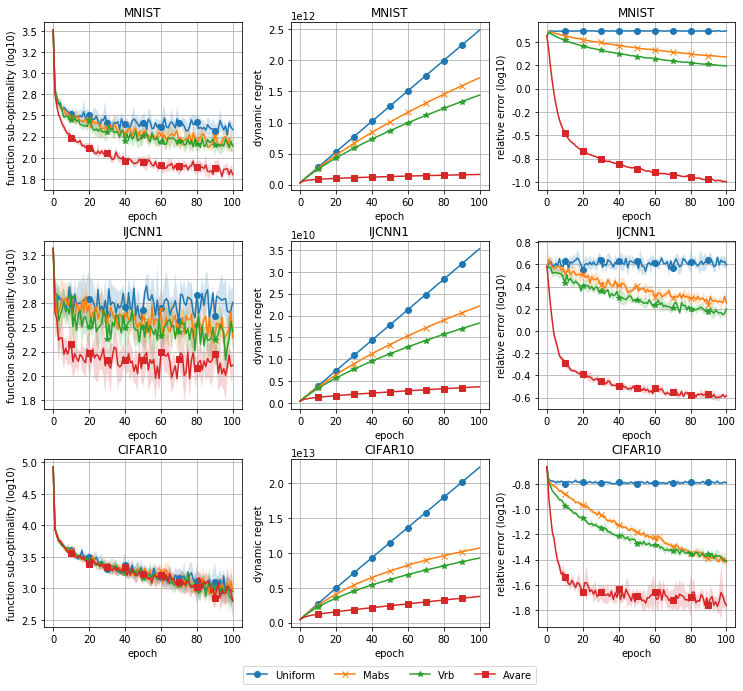
which ensures that . We ran the same experiment on MNIST, IJCNN1, and CIFAR10 as in Section 6, but with a constant step-size , and the epsilon sequence (23) with and , and . The results are displayed in figure 3, showing a similar performance compared to the decreasing step-sizes case. Note that choosing a too small can start to deteriorate the performance of the algorithm. It is still unclear how to set so as to guarantee good performance, but our experiments suggest that setting is a safe choice.
plain \bibliographysuppmendeley