This paper was converted on www.awesomepapers.org from LaTeX by an anonymous user.
Want to know more? Visit the Converter page.

Adaptive Inference for Change Points in High-Dimensional Data

Yangfan Zhang, Runmin Wang and Xiaofeng Shao 111 Yangfan Zhang is Ph.D. student, Xiaofeng Shao is Professor at Department of Statistics, University of Illinois at Urbana Champaign. Runmin Wang is Assistant Professor at Department of Statistical Science, Southern Methodist University. Emails: yangfan3@illinois.edu, runminw@mail.smu.edu and xshao@illinois.edu. We would like to thank two anonymous referees for constructive comments, which led to substantial improvements. We are also grateful to Dr. Farida Enikeeva for sending us the code used in Enikeeva and Harchaoui (2019). Shao’s research is partially supported by NSF-DMS 1807023 and NSF-DMS-2014018.

Abstract: In this article, we propose a class of test statistics for a change point in the mean of high-dimensional independent data. Our test integrates the U-statistic based approach in a recent work by Wang et al. (2019) and the LqL_{q}-norm based high-dimensional test in He et al. (2020), and inherits several appealing features such as being tuning parameter free and asymptotic independence for test statistics corresponding to even qqs. A simple combination of test statistics corresponding to several different qqs leads to a test with adaptive power property, that is, it can be powerful against both sparse and dense alternatives. On the estimation front, we obtain the convergence rate of the maximizer of our test statistic standardized by sample size when there is one change-point in mean and q=2q=2, and propose to combine our tests with a wild binary segmentation (WBS) algorithm to estimate the change-point number and locations when there are multiple change-points. Numerical comparisons using both simulated and real data demonstrate the advantage of our adaptive test and its corresponding estimation method.

Keywords: asymptotically pivotal, segmentation, self-normalization, structural break, U-statistics

1 Introduction

Testing and estimation of change points in a sequence of time-ordered data is a classical problem in statistics. There is a rich literature for both univariate and multivariate data of low dimension; see Csörgö and Horváth (1997), Chen and Gupta (2011) and Tartakovsky et al. (2014), for some book-length introductions and Perron (2006), Aue and Horváth (2013), and Aminikhanghahi and Cook (2017) for recent reviews of the subject. This paper addresses the testing and estimation for change points of high-dimensional data where the dimension pp is high and can exceed the sample size nn.

As high-dimensional data becomes ubiquitous due to technological advances in science, engineering and other areas, change point inference under the high-dimensional setting has drawn great interest in recent years. When the dimension pp is greater than sample size nn, traditional methods are often no longer applicable. Among recent work that addresses change point inference for the mean of high-dimensional data, we mention Horváth and Hušková (2012), Chan et al. (2013), Jirak (2015), Cho (2016), Wang and Samworth (2018), Enikeeva and Harchaoui (2019), Wang et al. (2019) and Yu and Chen (2020). In most of these papers, the proposed methods are powerful either when the alternative is sparse and strong, i.e., there are a few large non-zero values in the components of mean difference, or when the alternative is weak and dense, i.e., there are many small values in the components of mean difference. Among some of these papers, the sparsity appeared either explicitly in the assumptions, e.g. Wang and Samworth (2018), who proposed to project the data to some informative direction related to the mean change, to which univariate change point detection algorithm can be applied, or implicitly in the methodology, e.g. Jirak (2015), who took the maximal CUSUM statistic and therefore essentially targeted at the sparse alternative. Yu and Chen (2020) recently introduced a Gaussian multiplier bootstrap to calibrate critical values of the sup norm of CUSUM test statistics in high dimensions and their test is also specifically for sparse alternative. On the contrary, Horváth and Hušková (2012) aggregated the univariate CUSUM test statistics using the sum and their test is supposed to capture the dense alternative, but the validity of their method required the cross-sectional independence assumption. Wang et al. (2019) aimed at dense alternatives by extending the U-statistic based approach pioneered by Chen and Qin (2010) in the two-sample testing problem. An exception is the test developed in Enikeeva and Harchaoui (2019), which was based on a combination of a linear statistic and a scan statistic, and can be adaptive to both sparse and dense alternatives. However, its critical values were obtained under strong Gaussian and independent components assumptions and they do not seem to work when these assumptions are not satisfied; see Section 4 for numerical evidence.

In practice, it is often unrealistic to assume a particular type of alternative and there is little knowledge about the type of changes if any. Thus there is a need to develop new test that can be adaptive to different types of alternatives, and have good power against a broad range of alternatives. In this article, we shall propose a new class of tests that can have this adaptive power property, which holds without the strong Gaussian and independent components assumptions. Our test is built on two recent advances in the high-dimensional testing literature: Wang et al. (2019) and He et al. (2020). In Wang et al. (2019), they developed a mean change point test based on a U-statistic that is an unbiased estimator of the squared L2L_{2} norm of the mean difference. They further used the idea of self-normalization [see Shao (2010), Shao and Zhang (2010), Shao (2015)] to eliminate the need of estimating the unknown nuisance parameter. He et al. (2020) studied both one sample and two sample high-dimensional testing problem for the mean and covariance matrix using LqL_{q} norm, where q[2,]q\in[2,\infty] is some integer. They showed that the corresponding U-statistics at different qqs are asymptotically independent, which facilitates a simple combination of the tests based on several values of qq (say 22 and \infty) and their corresponding pp-values, and that the resulting combined test is adaptive to both dense and sparse alternatives.

Building on these two recent advances, we shall propose a new LqL_{q} norm based test for a change point in the mean of high-dimensional independent data. Our contributions to the literature is threefold. On the methodological front, we develop a new class of test statistics (as indexed by q2q\in 2\mathbb{N}) based on the principle of self-normalization in the high-dimensional setting. Our test is tuning parameter free when testing for a single change point. A simple combination of tests corresponding to different qqs can be easily implemented due to the asymptotic independence and results in an adaptive test that has well-rounded power against a wide range of alternatives. On the theory front, as He et al. (2020) proved the asymptotic independence of one-sample and two-sample U-statistics corresponding to different qqs, we derive the asymptotic independence for several stochastic processes corresponding to different qqs under significantly weaker assumptions. More precisely, we can define two-sample test statistics on different sub-samples for each q2q\in 2\mathbb{N}. These statistics can be viewed as smooth functionals of stochastic processes indexed by the starting and ending points of the sub-samples, which turn out to be asymptotically independent for different qqs. Compared to the adaptive test in Enikeeva and Harchaoui (2019), which relied on the Gaussian and independent components assumptions, our technical assumptions are much weaker, allowing non-Gaussianity and weak dependence among components. Furthermore, we obtained the convergence rate of the argmax of our SN-based test statistic standardized by sample size when there is one change point and q=2q=2. Lastly, in terms of empirical performance, we show in the simulation studies that the adaptive test can have accurate size and high power for both sparse and dense alternatives. Their power is always close to the highest one given by a single statistic under both dense and sparse alternatives.

The rest of the paper is organized as follows. In Section 2, we define our statistic, derive the limiting null distribution and analyze the asymptotic power when there is one change point. We also propose an adaptive procedure combining several tests of different q2q\in 2\mathbb{N}. In Section 3, we study the asymptotic behavior of change-point location estimators when there is a single change-point and combine the WBS algorithm with our test to estimate the location when there are multiple change points. In Section 4, we present some simulation results for both testing and estimation and apply the WBS-based estimation method to a real data set. Section 5 concludes. All technical details and some additional simulation results are gathered in the supplemental material.

2 Test Statistics and Theoretical Properties

Mathematically, let {Zt}t=1np\{Z_{t}\}_{t=1}^{n}\in\mathbb{R}^{p} be i.i.d random vectors with mean 0 and covariance Σ\Sigma. Our observed data is Xt=Zt+μtX_{t}=Z_{t}+\mu_{t}, where μt=E(Xt)\mu_{t}=E(X_{t}) is the mean at time tt. The null hypothesis is that there is no change point in the mean vector μt\mu_{t} and the alternative is that there is at least one change point, the location of which is unknown, i.e., we want to test

0:μ1=μ2==μnv.s1:μ1==μk1μk1+1==μksμks+1=μn,\mathcal{H}_{0}:\mu_{1}=\mu_{2}=\cdots=\mu_{n}\quad v.s\quad\mathcal{H}_{1}:\mu_{1}=\cdots=\mu_{k_{1}}\neq\mu_{k_{1}+1}=\cdots=\mu_{k_{s}}\neq\mu_{k_{s}+1}\cdots=\mu_{n},

where k1<k2<<ksk_{1}<k_{2}<\cdots<k_{s} and ss are unknown. Note that we assume temporal independence, which seems to be commonly adopted in change point analysis for genomic data; see Zhang et al. (2010), Jeng et al. (2010), and Zhang and Siegmund (2012) among others.

In this section, we first construct our two-sample U-statistic for a single change point alternative, which is the cornerstone for the estimation method we will introduce later. Then we derive the theoretical size and power results for our statistic. We also form an adaptive test that combines tests corresponding to different qqs. Throughout the paper, we assume pn+,p\wedge n\rightarrow+\infty, and we may use p=pnp=p_{n} to emphasize that pp can depend on nn. For a vector or matrix AA and q2q\in 2\mathbb{N}, we use Aq\|A\|_{q} to denote (i,jAijq)1/q\big{(}\sum_{i,j}A_{ij}^{q}\big{)}^{1/q}, and in particular, for q=2,q=Fq=2,\|\cdot\|_{q}=\|\cdot\|_{F} equals the Frobenius norm. We use Σs\|\Sigma\|_{s} to denote the spectral norm. Denote the number of permutations Pqk=k!/(kq)!P_{q}^{k}=k!/(k-q)!, and define \sum^{*} to be the summation over all pairwise distinct indices. If limnan/bn=0\lim_{n}a_{n}/b_{n}=0, we denote an=o(bn)a_{n}=o(b_{n}), and if 0<lim infnan/bnlim supnan/bn<+0<\liminf_{n}a_{n}/b_{n}\leq\limsup_{n}a_{n}/b_{n}<+\infty, we denote anbna_{n}\asymp b_{n}. Throughout the paper, we use “D\stackrel{{\scriptstyle D}}{{\rightarrow}}” to denote convergence in distribution, “P\stackrel{{\scriptstyle P}}{{\rightarrow}}” for convergence in probability, and “\leadsto” for process convergence in some suitable function space. We use ([0,1]3)\ell_{\infty}\left([0,1]^{3}\right) to denote the set of bounded functions on [0,1]3[0,1]^{3}.

2.1 U-statistic and Self-normalization

In this subsection, we shall develop our test statistics for one change point alternative, i.e.,

1:μ1==μk1μk1+1==μn,\mathcal{H}_{1}:\mu_{1}=\cdots=\mu_{k_{1}}\neq\mu_{k_{1}+1}=\cdots=\mu_{n},

where k1k_{1} is unknown. In Wang et al. (2019), a U-statistic based approach was developed and their test targets at the dense alternative since the power is a monotone function of nΔ2/ΣF1/2\sqrt{n}\|\Delta\|_{2}/\|\Sigma\|_{F}^{1/2}, where Δ\Delta is the difference between pre-break and post-break means, i.e., Δ=μnμ1\Delta=\mu_{n}-\mu_{1}, and Σ\Sigma is the covariance matrix of XiX_{i}. Thus their test may not be powerful if the change in mean is sparse and Δ2\|\Delta\|_{2} is small. Note that several tests have been developed to capture sparse alternatives as mentioned in Section 1. In practice, when there is no prior knowledge of the alternative for a given data set at hand, it would be helpful to have a test that can be adaptive to different types and magnitudes of the change. To this end, we shall adopt the LqL_{q} norm-based approach, as initiated by Xu et al. (2016) and He et al. (2020), and develop a class of test statistics indexed by q2q\in 2\mathbb{N}, and then combine these tests to achieve the adaptivity.

Denote Xi=(Xi,1,,Xi,p)TX_{i}=(X_{i,1},\ldots,X_{i,p})^{T}. For any positive even number q2q\in 2\mathbb{N}, consider the following two-sample U-statistic of order (q,q)(q,q),

Tn,q(k)=1PqkPqnkl=1p1i1,,iqkk+1j1,,jqn(Xi1,lXj1,l)(Xiq,lXjq,l),T_{n,q}(k)=\frac{1}{P_{q}^{k}P_{q}^{n-k}}\sum_{l=1}^{p}\sum^{*}_{1\leq i_{1},\ldots,i_{q}\leq k}\sum^{*}_{k+1\leq j_{1},\ldots,j_{q}\leq n}\left(X_{i_{1},l}-X_{j_{1},l}\right)\cdots\left(X_{i_{q},l}-X_{j_{q},l}\right),

for any k=q,,nqk=q,\cdots,n-q. Simple calculation shows that 𝔼[Tn,q(k)]=0\mathbb{E}\left[T_{n,q}(k)\right]=0 for any k=q,,nqk=q,\cdots,n-q under the null hypothesis, and 𝔼[Tn,q(k1)]=Δqq\mathbb{E}\left[T_{n,q}(k_{1})\right]=\|\Delta\|_{q}^{q} under the alternative. When q2+1q\in 2\mathbb{N}+1 (i.e., qq is odd) and under the alternative, 𝔼[Tn,q(k1)]=j=1pδjqΔqq\mathbb{E}\left[T_{n,q}(k_{1})\right]=\sum_{j=1}^{p}\delta_{j}^{q}\not=\|\Delta\|_{q}^{q} where Δ=(δ1,,δp)T\Delta=(\delta_{1},\cdots,\delta_{p})^{T}. This is the main reason we focus on the statistics corresponding to even qqs since for an odd qq, j=1pδjq=0\sum_{j=1}^{p}\delta_{j}^{q}=0 does not imply Δ=0\Delta=0.

If the change point location k1=τ1nk_{1}=\lfloor\tau_{1}n\rfloor, τ1(0,1)\tau_{1}\in(0,1) is known, then we would use Tn,q(k1)T_{n,q}(k_{1}) as our test statistic. As implied by the asymptotic results shown later, we have that under the null,

(τ1(1τ1)nΣq)q/2Tn,q(k1)q!DN(0,1),\left(\frac{\tau_{1}(1-\tau_{1})}{n\|\Sigma\|_{q}}\right)^{q/2}\frac{T_{n,q}(k_{1})}{\sqrt{q!}}\stackrel{{\scriptstyle D}}{{\rightarrow}}N(0,1),

under suitable moment and weak dependence assumptions on the components of XtX_{t}. In practice, a typical approach is to replace Σq\|\Sigma\|_{q} by a ratio-consistent estimator, which is available for q=2q=2 [see Chen and Qin (2010)], but not for general q2q\in 2\mathbb{N}. In practice, the location k1k_{1} is unknown, which adds additional complexity to the variance estimation and motivates Wang et al. (2019) to use the idea of self-normalization [Shao (2010), Shao and Zhang (2010)] in the case q=2q=2. Self-normalization is a nascent inferential method [Lobato (2001), Shao (2010)] that has been developed for low and fixed-dimensional parameter in a low dimensional time series. It uses an inconsistent variance estimator to yield an asymptotically pivotal statistic, and does not involve any tuning parameter or involves less number of tuning parameters compared to traditional procedures. See Shao (2015) for a comprehensive review of recent developments for low dimensional time series. There have been two recent extensions to the high-dimensional setting: Wang and Shao (2019) adopted a one sample U-statistic with trimming and extended self-normalization to inference for the mean of high-dimensional time series; Wang et al. (2019) used a two sample U-statistic and extended the self-normalization (SN)-based change point test in Shao and Zhang (2010) to high-dimensional independent data. Both papers are L2L_{2} norm based, and this seems to be the first time that a LqL_{q}-norm based approach is extended to high-dimensional setting via self-normalization.

Following Wang et al. (2019), we consider the following self-normalization procedure. Define

Un,q(k;s,m)\displaystyle U_{n,q}(k;s,m) =l=1psi1,,iqkk+1j1,,jqm(Xi1,lXj1,l)(Xiq,lXjq,l),\displaystyle=\sum_{l=1}^{p}\sum^{*}_{s\leq i_{1},\ldots,i_{q}\leq k}\sum^{*}_{k+1\leq j_{1},\ldots,j_{q}\leq m}\left(X_{i_{1},l}-X_{j_{1},l}\right)\cdots\left(X_{i_{q},l}-X_{j_{q},l}\right),

which is an un-normalized version of Tn,qT_{n,q} applied to the subsample (Xs,,Xm)(X_{s},\cdots,X_{m}). Let

Wn,q(k;s,m):=1ms+1t=s+q1kqUn,q(t;s,k)2+1ms+1t=k+qmqUn,q(t;k+1,m)2,W_{n,q}(k;s,m):=\frac{1}{m-s+1}\sum_{t=s+q-1}^{k-q}U_{n,q}(t;s,k)^{2}+\frac{1}{m-s+1}\sum_{t=k+q}^{m-q}U_{n,q}(t;k+1,m)^{2},

The self-normalized statistic is given by

T~n,q:=maxk=2q,,n2qUn,q(k;1,n)2Wn,q(k;1,n).\widetilde{T}_{n,q}:=\max_{k=2q,\ldots,n-2q}\frac{U_{n,q}(k;1,n)^{2}}{W_{n,q}(k;1,n)}.
Remark 2.1.

If we want to test for multiple change points, we can use the scanning idea presented in Zhang and Lavitas (2018) and Wang et al. (2019) and construct the following statistic:

Tn,q:=max2ql1l22qUn,q(l1;1,l2)2Wn,q(l1;1,l2)+maxm1+2q1m2n2qUn,q(m2;m1,n)2Wn,q(m2;m1,n).T_{n,q}^{*}:=\max_{2q\leq l_{1}\leq l_{2}-2q}\frac{U_{n,q}\left(l_{1};1,l_{2}\right)^{2}}{W_{n,q}\left(l_{1};1,l_{2}\right)}+\max_{m_{1}+2q-1\leq m_{2}\leq n-2q}\frac{U_{n,q}\left(m_{2};m_{1},n\right)^{2}}{W_{n,q}\left(m_{2};m_{1},n\right)}.

We shall skip further details as the asymptotic theory and computational implementation are fairly straightforward.

2.2 Limiting Null Distribution

Before presenting our main theorem, we need to make the following assumptions.

Assumption 2.1.

Suppose Z1,,ZnZ_{1},\ldots,Z_{n} are i.i.d. copies of Z0Z_{0} with mean 0 and covariance matrix Σ\Sigma, and the following conditions hold.

  1. 1.

    There exists c0>0c_{0}>0 not depending nn such that inf Vari=1,,pn(Z0,i)c0{}_{i=1,\ldots,p_{n}}\operatorname{Var}\left(Z_{0,i}\right)\geq c_{0}.

  2. 2.

    Z0Z_{0} has up to 88-th moments, with sup1jp𝔼[Z0,j8]C,\sup_{1\leq j\leq p}\mathbb{E}[Z_{0,j}^{8}]\leq C, and for h=2,,8h=2,\ldots,8 there exist constants ChC_{h} depending on hh only and a constant r>2r>2 such that

    |cum(Z0,l1,,Z0,lh)|Ch(1max1i,jh|lilj|)r.\left|\operatorname{cum}\left(Z_{0,l_{1}},\ldots,Z_{0,l_{h}}\right)\right|\leq C_{h}\left(1\vee\max_{1\leq i,j\leq h}\left|l_{i}-l_{j}\right|\right)^{-r}.
Remark 2.2 (Discussion of Assumptions).

The above cumulant assumption is implied by geometric moment contraction [cf. Proposition 2 of Wu and Shao (2004)] or physical dependence measure proposed by Wu (2005) [cf. Section 4 of Shao and Wu (2007)], or α\alpha-mixing [Andrews (1991), Zhurbenko and Zuev (1975)] in the time series setting. It basically imposes weak dependence among the pp components in the data. Our theory holds as long as a permutation of pp components satisfies the cumulant assumption, since our test is invariant to the permutation within the components.

To derive the limiting null distribution for T~n,q\widetilde{T}_{n,q}, we need to define some useful intermediate processes. Define

Dn,q(r;[a,b])\displaystyle D_{n,q}(r;[a,b]) =Un,q(nr;na+1,nb)\displaystyle=U_{n,q}(\lfloor nr\rfloor;\lfloor na\rfloor+1,\lfloor nb\rfloor)
=l=1pna+1i1,,iqnrnr+1j1,,jqnb(Xi1,lXj1,l)(Xiq,lXjq,l),\displaystyle=\sum_{l=1}^{p}\sum^{*}_{\lfloor na\rfloor+1\leq i_{1},\ldots,i_{q}\leq\lfloor nr\rfloor}\sum^{*}_{\lfloor nr\rfloor+1\leq j_{1},\ldots,j_{q}\leq\lfloor nb\rfloor}\left(X_{i_{1},l}-X_{j_{1},l}\right)\cdots\left(X_{i_{q},l}-X_{j_{q},l}\right),

for any 0a<r<b10\leq a<r<b\leq 1. Note that under the null, XiX_{i}’s have the same mean. Therefore, we can rewrite Dn,qD_{n,q} as

Dn,q(r;[a,b])=\displaystyle D_{n,q}(r;[a,b])= l=1pna+1i1,,iqnrnr+1j1,,jqbn(Xi1,lXj1,l)(Xiq,lXjq,l)\displaystyle\sum_{l=1}^{p}\sum^{*}_{\lfloor na\rfloor+1\leq i_{1},\ldots,i_{q}\leq\lfloor nr\rfloor}\sum^{*}_{\lfloor nr\rfloor+1\leq j_{1},\ldots,j_{q}\leq\lfloor bn\rfloor}\left(X_{i_{1},l}-X_{j_{1},l}\right)\cdots\left(X_{i_{q},l}-X_{j_{q},l}\right)
=\displaystyle= l=1pna+1i1,,iqnrnr+1j1,,jqbn(Zi1,lZj1,l)(Ziq,lZjq,l)\displaystyle\sum_{l=1}^{p}\sum^{*}_{\lfloor na\rfloor+1\leq i_{1},\ldots,i_{q}\leq\lfloor nr\rfloor}\sum^{*}_{\lfloor nr\rfloor+1\leq j_{1},\ldots,j_{q}\leq\lfloor bn\rfloor}\left(Z_{i_{1},l}-Z_{j_{1},l}\right)\cdots\left(Z_{i_{q},l}-Z_{j_{q},l}\right)
=\displaystyle= c=0q(1)qc(qc)PqcnrnacPcnbnrq+cSn,q,c(r;[a,b]).\displaystyle\sum_{c=0}^{q}(-1)^{q-c}\binom{q}{c}P^{\lfloor nr\rfloor-\lfloor na\rfloor-c}_{q-c}P^{\lfloor nb\rfloor-\lfloor nr\rfloor-q+c}_{c}S_{n,q,c}(r;[a,b]).

In the above expression, considering the summand for each c=0,1,,q,c=0,1,\ldots,q, we can define, for any 0a<r<b10\leq a<r<b\leq 1,

Sn,q,c(r;[a,b])=l=1pna+1i1,,icnrnr+1j1,,jqcnb(t=1cZit,ls=1qcZjs,l),S_{n,q,c}(r;[a,b])=\sum_{l=1}^{p}\sum^{*}_{\lfloor na\rfloor+1\leq i_{1},\cdots,i_{c}\leq\lfloor nr\rfloor}\sum^{*}_{\lfloor nr\rfloor+1\leq j_{1},\cdots,j_{q-c}\leq\lfloor nb\rfloor}\left(\prod_{t=1}^{c}Z_{i_{t},l}\prod_{s=1}^{q-c}Z_{j_{s},l}\right),

if nrna+1\lfloor nr\rfloor\geq\lfloor na\rfloor+1 and nbnr+1,\lfloor nb\rfloor\geq\lfloor nr\rfloor+1, and 0 otherwise.

Theorem 2.1.

If Assumption 2.1 holds, then under the null and for a finite set II of positive even numbers, we have that

{an,q1Sn,q,c(;[,])}qI,0cq{Qq,c(;[,])}qI,0cq\Big{\{}a_{n,q}^{-1}S_{n,q,c}(\cdot;[\cdot,\cdot])\Big{\}}_{q\in I,0\leq c\leq q}\leadsto\Big{\{}Q_{q,c}(\cdot;[\cdot,\cdot])\Big{\}}_{q\in I,0\leq c\leq q}

in ([0,1]3)\ell_{\infty}\left([0,1]^{3}\right) jointly over qI,0cqq\in I,0\leq c\leq q, where an,q=nql1,l2=1pΣl1,l2q=nqΣqqa_{n,q}=\sqrt{n^{q}\sum^{p}_{l_{1},l_{2}=1}\Sigma^{q}_{l_{1},l_{2}}}=\sqrt{n^{q}\|\Sigma\|_{q}^{q}}, and Qq,cQ_{q,c} are centered Gaussian processes. Furthermore, the covariance of Qq,c1Q_{q,c_{1}} and Qq,c2Q_{q,c_{2}} is given by

cov(Qq,c1(r1;[a1,b1]),Qq,c2(r2;[a2,b2]))=(Cc)c!(qc)!(rA)c(Rr)Cc(bR)qC,\operatorname{cov}\left(Q_{q,c_{1}}(r_{1};[a_{1},b_{1}]),Q_{q,c_{2}}(r_{2};[a_{2},b_{2}])\right)=\binom{C}{c}c!(q-c)!(r-A)^{c}(R-r)^{C-c}(b-R)^{q-C},

where (r,R)=(min{r1,r2},max{r1,r2})(r,R)=(\min\{r_{1},r_{2}\},\max\{r_{1},r_{2}\}),(a,A)=(min{a1,a2},max{a1,a2})(a,A)=(\min\{a_{1},a_{2}\},\max\{a_{1},a_{2}\}),(b,B)=(min{b1,b2},max{b1,b2}),(b,B)=(\min\{b_{1},b_{2}\},\\ \max\{b_{1},b_{2}\}), and (c,C)=(min{c1,c2},max{c1,c2})(c,C)=(\min\{c_{1},c_{2}\},\max\{c_{1},c_{2}\}). Additionally, Qq1,c1Q_{q_{1},c_{1}} and Qq2,c2Q_{q_{2},c_{2}} are mutually independent if q1q22q_{1}\neq q_{2}\in 2\mathbb{N}.

For illustration, consider the case when a1<a2<r1<r2<b1<b2a_{1}<a_{2}<r_{1}<r_{2}<b_{1}<b_{2} and c1c2c_{1}\leq c_{2}. We have

cov(Qq,c1(r1;[a1,b1]),Qq,c2(r2;[a2,b2]))=(c2c1)c1!(qc1)!(r1a2)c1(r2r1)c2c1(b1r2)qc2,\operatorname{cov}\left(Q_{q,c_{1}}(r_{1};[a_{1},b_{1}]),Q_{q,c_{2}}(r_{2};[a_{2},b_{2}])\right)=\binom{c_{2}}{c_{1}}c_{1}!(q-c_{1})!(r_{1}-a_{2})^{c_{1}}(r_{2}-r_{1})^{c_{2}-c_{1}}(b_{1}-r_{2})^{q-c_{2}},

which implies, for example,

var[Qq,c(r;[a,b])]=c!(qc)!(ra)c(br)qc.\operatorname{var}\left[Q_{q,c}(r;[a,b])\right]=c!(q-c)!(r-a)^{c}(b-r)^{q-c}.

The proof of Theorem 2.1 is long and is deferred to the supplement.

Theorem 2.2.

Suppose Assumption 2.1 holds. Then for a finite set II of positive even numbers,

{nqan,q1Dn,q(;[,])}qI{Gq(;[,])}qI\Big{\{}n^{-q}a_{n,q}^{-1}D_{n,q}(\cdot;[\cdot,\cdot])\Big{\}}_{q\in I}\leadsto\Big{\{}G_{q}(\cdot;[\cdot,\cdot])\Big{\}}_{q\in I}

in ([0,1]3)\ell_{\infty}\left([0,1]^{3}\right) jointly over qIq\in I, where

Gq=c=0q(1)qc(qc)(ra)qc(br)cQq,cG_{q}=\sum_{c=0}^{q}(-1)^{q-c}\binom{q}{c}(r-a)^{q-c}(b-r)^{c}Q_{q,c}

and Qq,cQ_{q,c} is given in Theorem 2.1. Furthermore, for q1q22q_{1}\not=q_{2}\in 2\mathbb{N}, Gq1G_{q_{1}} and Gq2G_{q_{2}} are independent. Consequently, we have that under the null,

T~n,q𝒟T~q=supr[0,1]Gq(r;0,1)20rGq(u;0,r)2𝑑u+r1Gq(u;r,1)2𝑑u.\widetilde{T}_{n,q}\stackrel{{\scriptstyle\mathcal{D}}}{{\longrightarrow}}\widetilde{T}_{q}=\sup_{r\in[0,1]}\frac{G_{q}(r;0,1)^{2}}{\int_{0}^{r}G_{q}(u;0,r)^{2}du+\int_{r}^{1}G_{q}(u;r,1)^{2}du}.

It can be derived that the Gq(;[,])G_{q}(\cdot;[\cdot,\cdot]) is a Gaussian process with the following covariance structure:

var[Gq(r;[a,b])]=c=0q(qc)2c!(qc)!(ra)2qc(br)q+c=q!(ra)q(br)q(ba)q.\operatorname{var}[G_{q}(r;[a,b])]=\sum^{q}_{c=0}\binom{q}{c}^{2}c!(q-c)!(r-a)^{2q-c}(b-r)^{q+c}=q!(r-a)^{q}(b-r)^{q}(b-a)^{q}.

When r1=r2=rr_{1}=r_{2}=r,

cov(Gq(r;[a1,b1]),Gq(r;[a2,b2]))=q!(rA)q(br)q(Ba)q.\displaystyle\operatorname{cov}(G_{q}(r;[a_{1},b_{1}]),G_{q}(r;[a_{2},b_{2}]))=q!(r-A)^{q}(b-r)^{q}(B-a)^{q}.

When r1r2r_{1}\not=r_{2},

cov(Gq(r1;[a1,b1]),Gq(r2;[a2,b2]))=q![(rA)(bR)(Ba)(Aa)(Rr)(Bb)]q,\operatorname{cov}(G_{q}(r_{1};[a_{1},b_{1}]),G_{q}(r_{2};[a_{2},b_{2}]))=q![(r-A)(b-R)(B-a)-(A-a)(R-r)(B-b)]^{q},

where (r,R,a,A,b,B,c,C)(r,R,a,A,b,B,c,C) is defined in Theorem 2.1. The limiting null distribution T~q\widetilde{T}_{q} is pivotal and its critical values can be simulated as done in Wang et al. (2019) for the case q=2q=2. The simulated critical values and their corresponding realizations for q=2,4,6q=2,4,6 are available upon request. For a practical reason, we did not pursue the larger qq, such as q=8,10q=8,10, since larger qq corresponds to more trimming on the two ends and the finite sample performance when q=6q=6 is already very promising for detecting sparse alternatives, see Section 4. An additional difficulty with larger qq is the associated computation cost and complexity in its implementation.

Remark 2.3.

Compared to He et al. (2020), we assume the 88th moment conditions, which is weaker than the uniform sub-Gaussian type conditions in their condition A.4(2), although the latter condition seems to be exclusively used for deriving the limit of the test statistic corresponding to q=q=\infty. Furthermore, since their strong mixing condition with exponential decay rate [cf. condition A.4(3) of He et al. (2020)] implies our cumulant assumption 2.1 [see Andrews (1991), Zhurbenko and Zuev (1975)], our overall assumption is weaker than condition A.4 in He et al. (2020). Despite the weaker assumptions, our results are stronger, as we derived the asymptotic independence of several stochastic process indexed by q2q\in 2\mathbb{N}, which implies the asymptotic independence of U-statistics indexed by q2q\in 2\mathbb{N}.

Note that our current formulation does not include the q=q=\infty case, which corresponds to LL_{\infty} norm of mean difference Δ\|\Delta\|_{\infty}. The LL_{\infty}-norm based test was developed by Yu and Chen (2020) and their test statistic is based on CUSUM statistics

Zn(s)=s(ns)n(1si=1sXi1nsi=s+1nXi)Z_{n}(s)=\sqrt{\frac{s(n-s)}{n}}\left(\frac{1}{s}\sum_{i=1}^{s}X_{i}-\frac{1}{n-s}\sum_{i=s+1}^{n}X_{i}\right)

and takes the form Tn=maxs0sns0Zn(s)T_{n}=\max_{s_{0}\leq s\leq n-s_{0}}\|Z_{n}(s)\|_{\infty}, where s0s_{0} is the boundary removal parameter. They did not obtain the asymptotic distribution of TnT_{n} but showed that a bootstrap CUSUM test statistic is able to approximate the finite sample distribution of TnT_{n} using a modification of Gaussian and bootstrap approximation techniques developed by Chernozhukov et al. (2013, 2017). Given the asymptotic independence between LqL_{q}-norm based U statistic and LL_{\infty}-norm based test statistic [He et al. (2020)] in the two-sample testing text, we would conjecture that TnT_{n} test statistic in Yu and Chen (2020) is asymptotically independent of our T~n,q\widetilde{T}_{n,q} for any q2q\in 2\mathbb{N} under suitable moment and weak componentwise dependence conditions. A rigorous investigation is left for future work.

2.3 Adaptive Test

Let II be a set of q2q\in 2\mathbb{N} (e.g. {2,6}). Since T~n,q\widetilde{T}_{n,q}s are asymptotically independent for different qIq\in I under the null, we can combine their corresponding pp-values and form an adaptive test. For example, we may use pada=minqIpqp_{ada}=\min_{q\in I}p_{q}, where pqp_{q} is the pp-value corresponding to T~n,q\widetilde{T}_{n,q}, as a new statistic. Its pp-value is equal to 1(1pada)|I|1-(1-p_{ada})^{|I|}. Suppose we want to perform a level-α\alpha test, it is equivalent to conduct tests based on T~n,q,qI\widetilde{T}_{n,q},\forall q\in I at level 1(1α)1/|I|1-(1-\alpha)^{1/|I|}, and reject the null if one of the statistics exceeds its critical value. Therefore, we only need to compare each T~n,q\widetilde{T}_{n,q} with its (1α)1/|I|(1-\alpha)^{1/|I|}-quantile of the corresponding limiting null distribution.

As we explained before, a smaller qq (say q=2q=2) tends to have higher power under the dense alternative, which is also the main motivation for the proposed method in Wang et al. (2019). On the contrary, a larger qq has a higher power under the sparse alternative, as limqΔnq=Δn\lim_{q\rightarrow\infty}\|\Delta_{n}\|_{q}=\|\Delta_{n}\|_{\infty}. Therefore, with the adaptive test, we can achieve high power under both dense and sparse alternatives with asymptotic size still equal to α\alpha. This adaptivity will be confirmed by our asymptotic power analysis presented in Section 2.4 and simulation results presented in Section 4.

2.4 Power Analysis

Theorem 2.3.

Assume that the change point location is at k1=τ1nk_{1}=\lfloor\tau_{1}n\rfloor with the change in the mean equal to Δn=(δn,1,,δn,p)T\Delta_{n}=(\delta_{n,1},\ldots,\delta_{n,p})^{T}. Suppose Assumption 2.1, and the following conditions on Δn\Delta_{n} hold. We have

  1. 1.

    If nq/2Δnqq/Σqq/2, then T~n,q𝒫n^{q/2}\left\|\Delta_{n}\right\|_{q}^{q}/\|\Sigma\|_{q}^{q/2}\rightarrow\infty,\text{ then }\widetilde{T}_{n,q}\stackrel{{\scriptstyle\mathcal{P}}}{{\longrightarrow}}\infty;

  2. 2.

    If nq/2Δnqq/Σqq/20, then T~n,q𝒟T~qn^{q/2}\left\|\Delta_{n}\right\|_{q}^{q}/\|\Sigma\|_{q}^{q/2}\rightarrow 0,\text{ then }\widetilde{T}_{n,q}\stackrel{{\scriptstyle\mathcal{D}}}{{\longrightarrow}}\widetilde{T}_{q};

  3. 3.

    If nq/2Δnqq/Σqq/2γ(0,+)n^{q/2}\left\|\Delta_{n}\right\|_{q}^{q}/\|\Sigma\|_{q}^{q/2}\rightarrow\gamma\in(0,+\infty), then

    T~n,q𝒟supr[0,1]{Gq(r;0,1)+γJq(r,0,1)}20r{Gq(u;0,r)+γJq(u,0,r)}2𝑑u+r1{Gq(u;r,1)+γJq(u,r,1)}2𝑑u,\widetilde{T}_{n,q}\stackrel{{\scriptstyle\mathcal{D}}}{{\longrightarrow}}\sup_{r\in[0,1]}\frac{\{G_{q}(r;0,1)+\gamma J_{q}(r,0,1)\}^{2}}{\int_{0}^{r}\{G_{q}(u;0,r)+\gamma J_{q}(u,0,r)\}^{2}du+\int_{r}^{1}\{G_{q}(u;r,1)+\gamma J_{q}(u,r,1)\}^{2}du},

    where

    Jq(r,a,b):={(τ1a)q(br)qa<τ1r<b(ra)q(bτ1)qa<r<τ1<b0τ1<a or τ1>b.J_{q}(r,a,b):=\left\{\begin{array}[]{lr}{\left(\tau_{1}-a\right)^{q}(b-r)^{q}}&{a<\tau_{1}\leq r<b}\\ {(r-a)^{q}\left(b-\tau_{1}\right)^{q}}&{a<r<\tau_{1}<b}\\ {0}&{\tau_{1}<a\text{ or }\tau_{1}>b}\end{array}\right..
Remark 2.4.

The following example illustrates the power behavior using different q2q\in 2\mathbb{N}. For simplicity, we assume Σ=Ip\Sigma=I_{p} and consider a change in the mean equal to Δn=δ(𝟏d,𝟎pd)T\Delta_{n}=\delta\cdot(\bm{1}_{d},\bm{0}_{p-d})^{T}. In addition to demonstrating that large (small) qq is favorable to the sparse (dense) alternatives, our local asymptotic power results stated in Theorem 2.3 also allow us to provide a rule to classify an alternative, which is given by

{sparsed=o(p)inbetweendpdensep=o(d).\left\{\begin{array}[]{lr}{sparse}&{d=o(\sqrt{p})}\\ {in~{}between}&{d\asymp\sqrt{p}}\\ {dense}&{\sqrt{p}=o(d)}\end{array}\right..

To have a nontrivial power, it suffices to have nq/2Δnqq/Σqq/2=dnq/2δq/p=γ(0,+)n^{q/2}\left\|\Delta_{n}\right\|_{q}^{q}/\|\Sigma\|_{q}^{q/2}=dn^{q/2}\delta^{q}/\sqrt{p}=\gamma\in(0,+\infty), which implies δ(p/d)1/qn1/2\delta\asymp(\sqrt{p}/d)^{1/q}n^{-1/2}. Therefore, when d=o(p)d=o(\sqrt{p}), a smaller δ\delta corresponds to a larger qq. On the contrary, when p=o(d)\sqrt{p}=o(d), a smaller qq that yields a larger δ\delta is preferable to have higher power. Similar argument still holds for more general Δn\Delta_{n} and Σ\Sigma, as long as we have a similar order for Δnqq\|\Delta_{n}\|_{q}^{q} and Σqq\|\Sigma\|_{q}^{q}, and the latter one is guaranteed by Assumption 2.1.

We can summarize the asymptotic powers of the tests under different alternatives in the following table. Note that when at least one single-qq based test obtains asymptotically nontrivial power (power 1), our adaptive test can also achieve nontrivial power (power 1).

Alternative δ\delta I={2}I=\{2\} I={q}I=\{q\} I={2,q}I=\{2,q\}
Dense p=o(d)\sqrt{p}=o(d) δ=o(p1/4d1/2n1/2)\delta=o(p^{1/4}d^{-1/2}n^{-1/2}) α\alpha α\alpha α\alpha
δp1/4d1/2n1/2\delta\asymp p^{1/4}d^{-1/2}n^{-1/2} β1(α,1)\beta_{1}\in(\alpha,1) α\alpha (α,β1)(\alpha,\beta_{1})
p1/4d1/2n1/2=o(δ),p^{1/4}d^{-1/2}n^{-1/2}=o(\delta), 1 α\alpha 1
& δ=o(p1/2qd1/qn1/2)\delta=o(p^{1/2q}d^{-1/q}n^{-1/2})
δp1/2qd1/qn1/2\delta\asymp p^{1/2q}d^{-1/q}n^{-1/2} 1 (α,1)(\alpha,1) 1
p1/2qd1/qn1/2=o(δ)p^{1/2q}d^{-1/q}n^{-1/2}=o(\delta) 1 1 1
Sparse d=o(pd=o(\sqrt{p}) δ=o(p1/2qd1/qn1/2)\delta=o(p^{1/2q}d^{-1/q}n^{-1/2}) α\alpha α\alpha α\alpha
δp1/2qd1/qn1/2\delta\asymp p^{1/2q}d^{-1/q}n^{-1/2} α\alpha β2(α,1)\beta_{2}\in(\alpha,1) (α,β2)(\alpha,\beta_{2})
p1/2qd1/qn1/2=o(δ),p^{1/2q}d^{-1/q}n^{-1/2}=o(\delta), α\alpha 1 1
& δ=o(p1/4d1/2n1/2)\delta=o(p^{1/4}d^{-1/2}n^{-1/2})
δp1/4d1/2n1/2\delta\asymp p^{1/4}d^{-1/2}n^{-1/2} (α,1)(\alpha,1) 1 1
p1/4d1/2n1/2=o(δ)p^{1/4}d^{-1/2}n^{-1/2}=o(\delta) 1 1 1
Table 1: Asymptotic powers of single-qq and adaptive tests

Liu et al. (2020) recently studied the detection of a sparse change in the high-dimensional mean vector under the Gaussian assumption as a minimax testing problem. Let ρ2=min(k1,nk1)Δn22\rho^{2}=\min(k_{1},n-k_{1})\|\Delta_{n}\|_{2}^{2}. In the fully dense case, i.e., when Δn0=p\|\Delta_{n}\|_{0}=p, where Δn0\|\Delta_{n}\|_{0} denotes the L0L_{0} norm, Theorem 8 in Liu et al. (2020) stated that the minimax rate is given by ρ2ΣFloglog(8n)Σsloglog(8n)\rho^{2}\asymp\|\Sigma\|_{F}\sqrt{\log\log(8n)}\vee\|\Sigma\|_{s}\log\log(8n). Thus under the assumption that k1/n=τ1(0,1)k_{1}/n=\tau_{1}\in(0,1), the L2L_{2}-norm based test in Wang et al. (2019) achieves the rate optimality up to a logarithm factor. Consequently, any adaptive test based on II is rate optimal (up to a logarithm factor) as long as 2I2\in I.

In the special case Σ=Ip\Sigma=I_{p}, the minimax rate is given by

ρ2{ploglog(8n) if dploglog(8n)dlog(eploglog(8n)d2)loglog(8n) if d<ploglog(8n).\rho^{2}\asymp\left\{\begin{array}[]{lr}\sqrt{p\log\log(8n)}&\text{ if }d\geq\sqrt{p\log\log(8n)}\\ d\log\left(\frac{ep\log\log(8n)}{d^{2}}\right)\vee\log\log(8n)&\text{ if }d<\sqrt{p\log\log(8n)}\end{array}\right..

Recall that Δn=δ(𝟏d,𝟎pd)T\Delta_{n}=\delta\cdot(\bm{1}_{d},\bm{0}_{p-d})^{T}. In the sparse setting d=o(p)d=o(\sqrt{p}) and under the assumptions that dpvd\asymp p^{-v},v(0,1/2)v\in(0,1/2) and d>loglog(8n)d>\log\log(8n), the minimax rate is dd (up to a logarithm factor), which corresponds to δn1/2\delta\asymp n^{-1/2}. Our LqL_{q}-norm based test is not minimax rate optimal since the detection boundary is (p/d)1/qn1/2(\sqrt{p}/d)^{1/q}n^{-1/2}, which gets closer to n1/2n^{-1/2} as q2q\in 2\mathbb{N} gets larger. In the dense setting p=o(d)\sqrt{p}=o(d) and under the assumptions that dpvd\asymp p^{-v},v(1/2,1)v\in(1/2,1) and d>ploglog(8n)d>\sqrt{p\log\log(8n)}, the minimax rate is p\sqrt{p} (up to a logarithm factor), which corresponds to δp1/4/nd\delta\asymp p^{1/4}/\sqrt{nd}. Therefore the L2L_{2}-norm based test in Wang et al. (2019) is again rate optimal (up to a logarithm factor).

3 Change-point Estimation

In this section, we investigate the change-point location estimation based on change-point test statistics we proposed in Section 2. Specifically, Section 3.1 presents convergence rate for the argmax of SN-based test statistic upon suitable standardization. Section 3.2 proposes a combination of wild binary segmentation (WBS, Fryzlewicz (2014)) algorithm with our SN-based test statistics for both single-qq test and adaptive test to estimate multiple change points.

3.1 Single Change-point Estimation

In this subsection, we propose to estimate the location of a change point assuming that the data is generated from the following single change-point model,

Xt=μ1+Δn𝟏(t>k)+Zt,t=1,,n,X_{t}=\mu_{1}+\Delta_{n}{\bf 1}(t>k^{*})+Z_{t},~{}t=1,\cdots,n,

where k=k1=τnk^{*}=k_{1}=\lfloor\tau^{*}n\rfloor is the location of change point. In the literature, it is common to focus on the convergence rate of the estimators of the relative location τ(0,1)\tau^{*}\in(0,1), that is, we shall focus on the convergence rate of τ^=k^/n\hat{\tau}=\hat{k}/n, where k^\hat{k} is an estimator for kk^{*}.

Given the discussions about size and power properties of the SN-based test statistic in Section 2, it is natural to use the argmax of the test statistic as the estimator for kk^{*}. That is, we define

k^=argmaxk=2q,,n2qUn,q(k;1,n)2Wn,q(k;1,n).\hat{k}=\operatorname{argmax}_{k=2q,\ldots,n-2q}\frac{U_{n,q}(k;1,n)^{2}}{W_{n,q}(k;1,n)}.

To present the convergence rate for τ^\hat{\tau}, we shall introduce the following assumptions.

Assumption 3.1.
  1. 1.

    tr(Σ4)=o(ΣF4)tr(\Sigma^{4})=o(\|\Sigma\|_{F}^{4});

  2. 2.

    l1,,lh=1pcum(Z0,l1,,Z0,lh)2CΣFh\sum_{l_{1},...,l_{h}=1}^{p}cum(Z_{0,l_{1}},...,Z_{0,l_{h}})^{2}\leq C\|\Sigma\|_{F}^{h}, for h=2,,6h=2,...,6;

  3. 3.

    ΣF=o(nΔn22)\|\Sigma\|_{F}=o(n\|\Delta_{n}\|_{2}^{2}).

Let γn,q=nq/2Δnqq/Σqq/2\gamma_{n,q}=n^{q/2}\|\Delta_{n}\|_{q}^{q}/\|\Sigma\|_{q}^{q/2} so γn,2=nΔn2/ΣF\gamma_{n,2}=n\|\Delta_{n}\|^{2}/\|\Sigma\|_{F}. We have the following convergence rate of τ^\hat{\tau} for the case q=2q=2.

Theorem 3.1.

Suppose Assumption 3.1 holds and q=2q=2. It holds that τ^τ=op(γn,21/4+κ)\hat{\tau}-\tau^{*}=o_{p}(\gamma_{n,2}^{-1/4+\kappa}) as npn\wedge p\rightarrow\infty, for any 0<κ<1/40<\kappa<1/4.

Remark 3.1.

Assumption 3.1 (1) and (2) have been assumed in Wang et al. (2019), and they are implied by Assumption 2.1; see Remark 3.2 in Wang et al. (2019). Assumption 3.1(3) is equivalent to γn,2\gamma_{n,2}\rightarrow\infty, which implies that τ^\hat{\tau} is a consistent estimator of τ\tau^{*}. Note that even in the low-dimensional setting, no convergence rate for the argmax of SN-based statistic (standarized by the sample size) is obtained in Shao and Zhang (2010). Thus this is the first time the asymptotic rate for the argmax of a SN-based test statistic is studied. On the other hand, the proof for the more general case q2q\in 2\mathbb{N} is considerably more involved than the special case q=2q=2 and is deferred to future investigation.

3.2 Multiple Change-point Estimation

In practice, the interest is often in the change point estimation or segmentation, when the presence of change points is confirmed by testing or based on prior knowledge. In the high-dimensional context, the literature on change point estimation is relatively scarce; see Cho (2016), Wang and Samworth (2018) and Wang et al. (2019). Here we shall follow the latter two papers and use the wild binary segmentation [Fryzlewicz (2014)] coupled with our test developed for a single qq or adaptive test to estimate the number and location of change points. Note that the standard binary segmentation procedure may fail when the change in means is not monotonic, as shown in Wang et al. (2019) via simulations.

For any integers s,es,e satisfying 2qs+2q1e2qn2q2q\leq s+2q-1\leq e-2q\leq n-2q, define

Qn,q(s,e):=maxb=s+2q1,,e2qUn,q2(b;s,e)Wn,q(b;s,e),Q_{n,q}(s,e):=\max_{b=s+2q-1,...,e-2q}\frac{U_{n,q}^{2}(b;s,e)}{W_{n,q}(b;s,e)},

Note that Qn,q(s,e)Q_{n,q}(s,e) is essentially the statistic Tn,qT_{n,q} based on the sub-sample (Xs,,Xe)(X_{s},...,X_{e}). Denote a random sample of (sm,em)(s_{m},e_{m}) s.t. 2qsm+2q1em2qn2q2q\leq s_{m}+2q-1\leq e_{m}-2q\leq n-2q as FnMF_{n}^{M}, where the sample is drawn independently with replacement of size MM. In practice, we may require the segments to be slightly longer to reduce unnecessary fluctuations of the critical values. Then define ξ^n,M,q=maxm=1,,MQn,q(sm,em)\hat{\xi}_{n,M,q}=\max_{m=1,\cdots,M}Q_{n,q}(s_{m},e_{m}) and we stop the algorithm if ξ^n,M,qξn,q\hat{\xi}_{n,M,q}\leq\xi_{n,q}, where ξn,q\xi_{n,q} is some threshold to be specified below, and estimate the change point otherwise; see Algorithm 1 for details.

One anonymous reviewer asked whether it is possible to derive the limiting distribution of ξ^n,M,q\hat{\xi}_{n,M,q} under the null, which turns out to be challenging for two reasons: (1) The SN-based test statistic for different intervals could be highly dependent, especially when the two intervals overlap by a lot; (2) the number of such randomly generated intervals is usual large, and it would be more valuable to develop an asymptotic distribution under the assumption that both sample size and number of intervals go to infinity. It seems difficult to use the classical argument for this problem, and we shall leave this for future investigation.

To obtain the threshold value ξn,q\xi_{n,q} as needed in the Algorithm 1, we generate RR standard Gaussian samples each of which has sample size nn and dimension pp. For the rr-th sample (r=1,,R)r=1,\ldots,R), we calculate

ξ^n,M,q(r)=maxm=1,,MQn,q(r)(sm,em),\hat{\xi}^{(r)}_{n,M,q}=\max_{m=1,\cdots,M}Q_{n,q}^{(r)}(s_{m},e_{m}),

where Qn,q(r)(sm,em)Q_{n,q}^{(r)}(s_{m},e_{m}) is the SN-based test statistic applied to the rrth Gaussian simulated sample. We can take ξn,q\xi_{n,q} to be the 95% quantile of {ξ^n,M,q(r)}r=1R\{\hat{\xi}^{(r)}_{n,M,q}\}_{r=1}^{R}. Since the self-normalized test statistic is asymptotically pivotal, the above threshold ξn,q\xi_{n,q} is expected to approximate the 95% quantile of the finite sample distribution of maximized SN-based test statistic applied to MM randomly drawn sub-samples from the original data.

1:function WBS(S,ES,E)
2:     if ES<4q1E-S<4q-1 then
3:         STOP
4:     else
5:         s,e\mathcal{M}_{s,e}\leftarrow set of those 1mM1\leq m\leq M s.t. Ssm,emE,emsm4q1S\leq s_{m},e_{m}\leq E,e_{m}-s_{m}\geq 4q-1
6:         mqm_{q}\leftarrowargmaxQn,qms,e(sm,em){}_{m\in\mathcal{M}_{s,e}}Q_{n,q}(s_{m},e_{m})
7:         if Qn,q(smq,emq)>ξn,qQ_{n,q}(s_{m_{q}},e_{m_{q}})>\xi_{n,q} then
8:              add b0b_{0}\leftarrowargmaxUn,qb(b;smq,emq)/Wn,q(b;smq,emq){}_{b}U_{n,q}(b;s_{m_{q}},e_{m_{q}})/W_{n,q}(b;s_{m_{q}},e_{m_{q}}) to set of estimated CP
9:              WBS(S,b0)(S,b_{0})
10:              WBS(b0+1,E)(b_{0}+1,E)
11:         else
12:              STOP               
Algorithm 1 WBS Algorithm for a given q2q\in 2\mathbb{N}

To apply the adaptive test, we calculate ξ^n,M,q(r)\hat{\xi}_{n,M,q}^{(r)} with rr-th sample using different qIq\in I. Denote qI:=maxqIqq_{I}:=\max_{q\in I}q We calculate pp-value for each single-qq based statistic and select the most significant one for location estimation, which gives the adaptive version; see Algorithm 2.

1:function WBS(S,ES,E)
2:     if ES<4qI1E-S<4q_{I}-1 then
3:         STOP
4:     else
5:         p0=0.05p_{0}=0.05
6:         for qq in II do
7:              s,e\mathcal{M}_{s,e}\leftarrow set of those 1mM1\leq m\leq M s.t. Ssm,emE,emsm4qI1S\leq s_{m},e_{m}\leq E,e_{m}-s_{m}\geq 4q_{I}-1
8:              mqm_{q}\leftarrowargmaxQn,qms,e(sm,em){}_{m\in\mathcal{M}_{s,e}}Q_{n,q}(s_{m},e_{m})
9:              pq=R1#{Qn,q(smq,emq)>ξn,M,q(r)}r=1Rp_{q}=R^{-1}\#\Big{\{}Q_{n,q}(s_{m_{q}},e_{m_{q}})>\xi^{(r)}_{n,M,q}\Big{\}}_{r=1}^{R}
10:              if pq<p0p_{q}<p_{0} for current qq then
11:                  b0b_{0}\leftarrowargmaxUn,qb(b;smq,emq)/Wn,q(b;smq,emq){}_{b}U_{n,q}(b;s_{m_{q}},e_{m_{q}})/W_{n,q}(b;s_{m_{q}},e_{m_{q}})
12:                  p0pqp_{0}\leftarrow p_{q}
13:                  NEXT                        
14:         add b0b_{0} to set of estimated CP
15:         WBS(S,b0)(S,b_{0})
16:         WBS(b0+1,E)(b_{0}+1,E)      
Algorithm 2 Adaptive WBS Algorithm

4 Numerical Studies

In this section, we present numerical results to examine the finite sample performance of our testing and estimation method in comparison with the existing alternatives. Section 4.1 shows the size and power for the single change point tests; Section 4.2 presents the estimation result when there is one single change-point; Section 4.3 compares several WBS-based estimation methods for multiple change point estimation, including the INSPECT method in Wang and Samworth (2018). Finally, we apply our method to a real data set in Section 4.4.

4.1 Single Change Point Testing

In this subsection, we examine the size and power property of our single-qq and adaptive tests in comparison with the one in Enikeeva and Harchaoui (2019) (denoted as EH), which seems to be the only adaptive method in the literature. The data XiN(μi,Σ)X_{i}\sim N(\mu_{i},\Sigma), where μi=0\mu_{i}=0 for i=1,,ni=1,\cdots,n under the null. We set (n,p)=(200,100)(n,p)=(200,100) and (400,200)(400,200) and performed 2000 Monte carlo replications. We consider four different configurations of Σ=(σij)\Sigma=(\sigma_{ij}) as follows,

σij={𝟙i=jId0.5|ij|AR(0.5)0.8|ij|AR(0.8)𝟙i=j+0.25𝟙ijCS.\sigma_{ij}=\left\{\begin{array}[]{lr}{\mathds{1}_{i=j}}&{\text{Id}}\\ {0.5^{|i-j|}}&{\text{AR(0.5)}}\\ {0.8^{|i-j|}}&{\text{AR(0.8)}}\\ {\mathds{1}_{i=j}+0.25\cdot\mathds{1}_{i\not=j}}&{\text{CS}}\\ \end{array}\right..

They correspond to independent components (Id), auto-regressive model with order 11 (AR(0.5) and AR(0.8)) and compound symmetric (CS), respectively. The first three configurations imply weak dependence among components so satisfy Assumption 2.1, whereas the compound symmetric covariance matrix corresponds to strong dependence among components and violates our assumption. The size of our tests, including T~n,q\widetilde{T}_{n,q} at a single q=2,4,6q=2,4,6 and combined tests with =(2,4)\mathcal{I}=(2,4), (2,6)(2,6) and (2,4,6)(2,4,6) are presented in Table 2. It appears that all tests are oversized when Σ\Sigma is compound symmetric, which is somewhat expected since the strong dependence among components brings non-negligible errors in asymptotic approximation. As a matter of fact, we conjecture that our limiting null distribution T~q\widetilde{T}_{q} no longer holds in this case. Below we shall focus our comments on the first three configurations (Id, AR(0.5) and AR(0.8)).

The size for q=2q=2 (i.e., the test in Wang et al. (2019)) appears quite accurate except for some degree of under-rejection in the Id case. For q=4q=4, it is oversized and its size seems inferior to the case q=6q=6, which also shows some over-rejection for the AR(1) models when (n,p)=(200,100)(n,p)=(200,100), but the size distortion improves quite a bit when we increase (n,p)(n,p) to (400,200)(400,200). Among the three combined tests, there are apparent over-rejections for =(2,4)\mathcal{I}=(2,4), (2,4,6)(2,4,6) for the AR(1) models, and the test corresponding to =(2,6)\mathcal{I}=(2,6) exhibits the most accurate size overall. By contrast, the EH shows serious size distortions in all settings with some serious over-rejection when the componentwise dependence is strong (e.g., AR(0.8) and CS), which is consistent with the fact that its validity strongly relies on the Gaussian and componentwise independence assumptions. We also checked the sensitivity of the size with respect to nonGaussian assumptions and observe serious distortion for EH when the data is generated from a nonGaussian distribution (results not shown). Overall, the adaptive test with =(2,6)\mathcal{I}=(2,6) seems preferred to all other tests (including the adaptive test with =(2,4,6)\mathcal{I}=(2,4,6)) in terms of size accuracy.

Please insert Table 2 here!

To investigate the power, we let μi=0\mu_{i}=0 for in/2i\leq n/2 and μi=δ/d(𝟏d,𝟎pd)T\mu_{i}=\sqrt{\delta/d}\cdot(\bm{1}_{d},\bm{0}_{p-d})^{T} for i>n/2i>n/2. We take δ=1,2\delta=1,2 and d=3d=3, which corresponds to a sparse alternative; and let d=pd=p to examine the power under the dense alternative; see Table 3. In the case of sparse alternative, we can see that the powers corresponding to q=4q=4 and q=6q=6 are much higher than that for q=2q=2, which is consistent with our intuition. When q=4q=4, the power is slightly higher than that for q=6q=6, which might be explained by the over-rejection with q=4q=4 (in the case of AR(1) models), and we expect no power gain as we increase qq to 8,108,10 etc, so the results for these larger qq are not included. Also for larger qq, there is more trimming involved as the maximum runs from 2q2q to n2qn-2q in our test statistics, so if the change point occurs outside of the range [2q,n2q][2q,n-2q], our test has little power. In the dense alternative case, the power for q=2q=2 is the highest as expected, and the power for q=4q=4 is again slightly higher than that for q=6q=6.

The power of the combined tests (i.e., =(2,4){\mathcal{I}}=(2,4) or (2,6)(2,6) or (2,4,6)(2,4,6)) is always fairly close to the best single one within the set. For example, the power for (2,6)(2,6) is very close to the power for q=6q=6 in the sparse case and is quite close to the power for q=2q=2 in the dense case, indicating the adaptiveness of the combined test. In the sparse case, the powers for =(2,4){\mathcal{I}}=(2,4) and (2,4,6)(2,4,6) are slightly higher than that for (2,6)(2,6), which could be related to the over-rejection of the tests with =(2,4){\mathcal{I}}=(2,4) and (2,4,6)(2,4,6), especially when the data is generated from AR(1) models. Overall, the adaptive tests (i.e., (2,4), (2,6) or (2,4,6)) have a good all-around power behavior against both sparse and dense alternatives and are preferred choices when there is no prior knowledge about the type of alternative the data falls into. Since the size for (2,6)(2,6) is more accurate than that for (2,4) and (2,4,6), we slightly favor the (2,6)(2,6) combination. EH exhibits high power for all settings, but it is at the cost of serious size distortion. We shall not present size-adjusted power as the serious distortion is too great to recommend its use when there are componentwise dependence in the data.

Please insert Tables 3 here!

4.2 Estimation for Single Change-point

In this subsection, we present the square root of mean-square-error (RMSE, multiplied by 1000 for readability) of SN-based location estimators and compare with the EH-based estimator under the same settings as we used in Section 4.1.

For both dense and sparse alternatives, the proposed estimators (i.e., SN(2), SN(4) and SN(6)) perform better than the EH method when the signal is relatively weak (i.e., δ=1,2\delta=1,2). However, as the signal becomes stronger (i.e., δ=4\delta=4), the EH method can outperform ours in the identity covariance matrix case. On the other other hand, the performance of the EH estimator apparently deterioates as the cross-sectional dependence gets stronger, indicating its strong reliance on the componentwise independence assumption. It is interesting to note that the SN-based method performs fairly well, even in the case of compound symmetric covariane matrix, and SN(6) outperforms the other two in all settings. A theoretical justification for the latter phenomenon would be intriguing.

Please insert Tables 4 here!

4.3 Estimation for Multiple Change Points

In the following simulations, we compare our WBS-based method with the INSPECT method proposed by Wang and Samworth (2018). Following Wang et al. (2019), we generate 100 samples of i.i.d. standard normal variables {Zt}t=1n\{Z_{t}\}_{t=1}^{n} with n=120,p=50n=120,p=50. The 3 change points are located at 30,6030,60 and 9090. Denote the changes in mean by 𝜽𝟏,𝜽𝟐,𝜽𝟑,\bm{\theta_{1}},\bm{\theta_{2}},\bm{\theta_{3}}, with 𝜽𝟏=𝜽𝟐=2k1/d1(𝟏d1,𝟎pd1),𝜽𝟑=2k2/d2(𝟏d2,𝟎pd2)\bm{\theta_{1}}=-\bm{\theta_{2}}=2\sqrt{k_{1}/d_{1}}\cdot(\bm{1}_{d_{1}},\bm{0}_{p-d_{1}}),\bm{\theta_{3}}=2\sqrt{k_{2}/d_{2}}\cdot(\bm{1}_{d_{2}},\bm{0}_{p-d_{2}}). We use, e.g., Dense(2.5) to denote dense changes with di=p=50,ki=2.5d_{i}=p=50,k_{i}=2.5 for i=1,2,3i=1,2,3 and Sparse(4) to denote sparse changes with di=5,ki=4d_{i}=5,k_{i}=4 for i=1,2,3i=1,2,3. In particular, Dense(2.52.5) & Sparse(44) refers to k1=2.5,k2=4,d1=5,d2=50k_{1}=2.5,k_{2}=4,d_{1}=5,d_{2}=50, where we have a mixture of dense and sparse changes.

We compare WBS with INSPECT, for which we use default parameters with the ”InspectChangepoint” package in R. We use 2 different metrics for evaluating the performance of different methods. One is to calculate the mean square errors (MSE) of the estimated number of change points. The other metric takes the accuracy of location estimation into account. We utilize the correlated rand index (CRI), which can measure the accuracy of change point location estimation. See Rand (1971), Hubert and Arabie (1985) and Wang et al. (2019) for more details. For perfect estimation, the calculated CRI is 1. In general it is a number between 0 and 1 and the more precise we estimate the change point locations, the higher CRI we get. We average the CRI for all Monte Carlo replications and record the average rand index (ARI). We report the MSE and ARI of different methods based on 100 replications in Table 5.

When there are only sparse changes and δ=2.5\delta=2.5, the performance of adaptive procedure (WBS(2,6)) is similar to WBS(6), whose estimation is much more accurate than WBS(2) and INSPECT. When we strengthen the signal by increasing δ\delta from 2.52.5 to 44, the detection power of all methods increase, but instead INSPECT has the best estimation accuracy in this case, closely followed by WBS(6) and WBS(2,6). In the case of purely dense changes with δ=2.5\delta=2.5, the performance of WBS(2) dominates the others and WBS(2,6) is the second best. When we increase δ\delta from 2.52.5 to 44 in this setting, the adaptive test slightly outperforms INSPECT, and its performance is comparable to WBS(2). For both dense settings, the performance of WBS(6) is rather poor. We can see that under all these four settings, the performance of WBS(2,6) is always close to the best, indicating its adaptiveness to different types of change points. Moreover, when there is a mixture of dense and sparse changes, the adaptive method outperforms all the others. In practice, the type of changes is often unknown, and therefore our adaptive procedure could be appealing for practitioners.

Please insert Table 5 here!

4.4 Real data illustration

In this subsection, we study the genomic micro-array data set that contains log intensity ratios of 43 individuals with bladder tumor, measured at 2215 different loci. The data was available in R package ecp and was also studied by Wang et al. (2019) and Wang and Samworth (2018). We compare our results with theirs.

We take the first 200 loci for our study. For the WBS algorithm, we generate 10000 samples from i.i.d. standard normal distributions with (n,p)=(200,43)(n,p)=(200,43), and draw 5000 random intervals to calculate the supremum statistics and get the 98%-quantile as our critical value. The change points detected by WBS at 0.98 level and the 20 most significant points detected by INSPECT are given as follows.

q=233,39,46,74,97,102,135,155,173,191q=615,32,44,59,74,91,116,134,158,173,186q=2,615,32,38,44,59,74,91,97,102,116,134,158,173,186,191INSPECT15,26,28,33,36,40,56,73,91,97,102,119,131,134,135,146,155,174,180,191\begin{array}[]{ll}q=2&33,39,46,74,97,102,135,155,173,191\\ q=6&15,32,44,59,74,91,116,134,158,173,186\\ q=2,6&15,32,38,44,59,74,91,97,102,116,134,158,173,186,191\\ \text{INSPECT}&15,26,28,33,36,40,56,73,91,97,102,119,131,134,135,146,155,174,180,191\end{array}

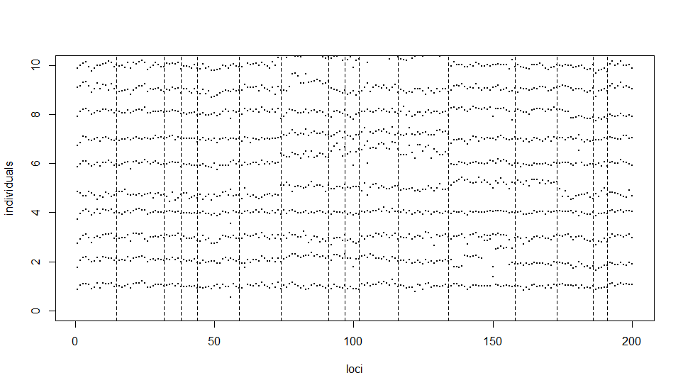
We can see that the set of change points detected by the adaptive WBS method is roughly a union of the sets corresponding to two single WBS methods (that is, for a single qq), which suggests that the adaptive WBS method captures both sparse and dense alternatives as expected. In particular, 32(33),44(46),74,134(135), 158(155),173 are detected by both single methods, 38(39),97,102,191 are detected only by q=2q=2, and 15, 59, 91,116,186 only by q=6q=6. The set of the change points detected by adaptive WBS method overlaps with the set for INSPECT by a lot, including 15, 32(33), 38(36), 74(73), 91, 97, 102, 116(119), 134, 158(155), 173(174), and 191. It is worth noting that the change points at locations 91, 97, 191 were only detected by one of two single WBS methods and INSPECT, whereas the adaptive WBS method is able to capture with its good all-round power property again a broad range of alternatives. In Figure 1, we plot the log intensity ratios of the first 10 individuals at first 200 loci, and the locations of the change points estimated by the adaptive method.

Please insert Figure 1 here!

This example clearly demonstrates the usefulness of the proposed adaptive test and corresponding WBS-based estimation method. An important practical choice is the threshold, which can be viewed as a tuning parameter in the implementation of WBS algorithm. We shall leave its choice for future investigation.

5 Conclusion

In this paper, we propose a class of asymptotically pivotal statistics for testing a mean change in high-dimensional independent data. The test statistics are formed on the basis of an unbiased estimator of qq-th power of the LqL_{q} norm of the mean change via U-statistic and self-normalization. They are asymptotically independent for different q2q\in 2\mathbb{N}, and therefore, we can form an adaptive test by taking the minimum of pp-values corresponding to test statistics indexed by q2q\in 2\mathbb{N}. The resulting test is shown to have good overall power against both dense and sparse alternatives via theory and simulations. On the estimation front, we obtain the convergence rate for the argmax of SN-based test statistic standardized by sample size under the one change-point model and q=2q=2. We also combine our tests with WBS algorithm to estimate multiple change points. As demonstrated by our simulations, the WBS-based estimation method inherits the advantage of the adaptive test, as it outperforms other methods under the setting where there is a mixture of dense and sparse change points, and has close-to-best performance for purely dense and purely sparse cases.

To conclude, we mention that it would be interesting to extend our adaptive test to the high-dimensional time series setting, for which a trimming parameter seems necessary to accommodate weak temporal dependence in view of recent work by Wang and Shao (2019). In addition, the focus of this paper is on mean change, whereas in practice the interest could be on other high-dimensional parameters, such as vector of marginal quantiles, variance-covariance matrix, and even high-dimensional distributions. It remains to be seen whether some extensions to these more general parameters are possible in the high-dimensional environment. We shall leave these open problems for future research.

DGP (n,p)(n,p) α=\alpha=5%
q=2q=2 q=4q=4 q=6q=6 q=2,4q=2,4 q=2,6q=2,6 q=2,4,6q=2,4,6 EH
Id (200,100) 0.028 0.065 0.056 0.052 0.032 0.045 0.01
(400,200) 0.036 0.068 0.051 0.055 0.041 0.045 0
AR(0.5) (200,100) 0.049 0.109 0.077 0.087 0.063 0.085 0.111
(400,200) 0.043 0.089 0.058 0.081 0.056 0.074 0.093
AR(0.8) (200,100) 0.051 0.12 0.079 0.097 0.063 0.086 0.613
(400,200) 0.045 0.094 0.046 0.082 0.047 0.069 0.66
CS (200,100) 0.095 0.103 0.081 0.109 0.088 0.098 0.729
(400,200) 0.11 0.085 0.061 0.116 0.099 0.104 0.898
Table 2: Size for one change point test
1\mathcal{H}_{1} DGP δ\delta (n,p)(n,p) α=\alpha=5%
q=2q=2 q=4q=4 q=6q=6 q=2,4q=2,4 q=2,6q=2,6 q=2,4,6q=2,4,6 EH
Sparse Id 1 (200,100) 0.742 0.981 0.962 0.982 0.967 0.981 0.844
(400,200) 0.94 1 1 1 1 1 0.998
2 (200,100) 0.995 1 1 1 1 1 1
(400,200) 1 1 1 1 1 1 1
AR(0.5) 1 (200,100) 0.566 0.947 0.91 0.933 0.894 0.93 0.809
(400,200) 0.82 1 1 1 0.996 1 0.994
2 (200,100) 0.94 1 1 1 0.999 1 0.999
(400,200) 0.998 1 1 1 1 1 1
AR(0.8) 1 (200,100) 0.298 0.887 0.84 0.883 0.82 0.876 0.912
(400,200) 0.522 0.99 0.994 0.99 0.988 0.992 1
2 (200,100) 0.703 0.997 0.995 0.997 0.994 0.997 0.994
(400,200) 0.928 1 1 1 1 1 1
CS 1 (200,100) 0.231 0.971 0.937 0.966 0.927 0.962 0.964
(400,200) 0.226 1 1 1 1 1 1
2 (200,100) 0.592 1 1 1 1 1 1
(400,200) 0.656 1 1 1 1 1 1
Dense Id 1 (200,100) 0.718 0.326 0.292 0.677 0.661 0.645 0.444
(400,200) 0.94 0.348 0.282 0.912 0.896 0.89 0.82
2 (200,100) 0.995 0.567 0.612 0.991 0.99 0.985 0.978
(400,200) 1 0.682 0.628 1 1 1 1
AR(0.5) 1 (200,100) 0.589 0.357 0.312 0.581 0.554 0.552 0.566
(400,200) 0.808 0.36 0.338 0.762 0.754 0.732 0.832
2 (200,100) 0.927 0.616 0.573 0.917 0.909 0.899 0.93
(400,200) 0.994 0.68 0.608 0.99 0.988 0.984 0.998
AR(0.8) 1 (200,100) 0.385 0.33 0.262 0.41 0.358 0.376 0.831
(400,200) 0.502 0.32 0.242 0.474 0.436 0.422 0.912
2 (200,100) 0.693 0.537 0.474 0.699 0.656 0.667 0.94
(400,200) 0.872 0.564 0.51 0.866 0.848 0.84 0.986
CS 1 (200,100) 0.345 0.277 0.235 0.363 0.33 0.338 0.84
(400,200) 0.36 0.284 0.214 0.368 0.334 0.348 1
2 (200,100) 0.544 0.455 0.414 0.551 0.526 0.532 0.919
(400,200) 0.588 0.474 0.424 0.584 0.55 0.562 1
Table 3: Power for one change point test under different alternatives
δ\delta Method Sparse Dense
Id AR(0.5) AR(0.8) CS Id AR(0.5) AR(0.8) CS
1 SN(2) 38.7 53.7 72.3 84.5 41.1 50.6 72.6 91.4
SN(4) 20.3 24.5 26.7 20.9 44.6 43.0 49.1 49.6
SN(6) 18.5 22.0 22.3 19.6 33.1 31.6 32.6 31.4
EH 150.3 214.9 300.6 326.8 155.6 216.9 291.3 332.3
2 SN(2) 26.0 33.5 41.7 44.3 27.5 36.6 54.8 76.8
SN(4) 14.4 17.5 19.6 16.3 37.9 38.3 45.8 48.8
SN(6) 12.1 14.1 14.9 11.9 29.7 28.6 31.9 30.5
EH 41.4 90.2 196.8 272.7 40.1 110.8 210.2 286.6
4 SN(2) 21.8 24.8 29.5 30.4 20.7 26.1 39.2 64.2
SN(4) 12.1 14.7 16.5 14.1 22.8 27.8 39.0 44.3
SN(6) 9.9 10.8 11.6 10.1 26.1 26.5 29.1 33.6
EH 8.7 16.7 66.8 153.2 9.7 29.9 109.4 209.6
Table 4: RMSE (multiplied by 10310^{3}) for one change point location estimation under different alternatives
Refer to caption
Figure 1: ACGH data of the first 10 individuals at first 200 loci. The dashed lines represent the locations of the change points detected.
N^N\hat{N}-N MSE ARI
-3 -2 -1 0 1 2 3
Sparse(2.5) WBS-SN(2) 0 1 11 75 13 0 0 0.28 0.8667
WBS-SN(4) 0 0 0 98 2 0 0 0.02 0.958
WBS-SN(6) 0 0 0 94 5 1 0 0.09 0.9552
WBS-SN(2,6) 0 0 0 90 10 0 0 0.1 0.9489
INSPECT 0 26 0 69 5 0 0 1.09 0.7951
Sparse(4) WBS-SN(2) 0 0 0 86 14 0 0 0.14 0.9188
WBS-SN(4) 0 0 0 98 2 0 0 0.02 0.9684
WBS-SN(6) 0 0 0 94 5 1 0 0.09 0.9707
WBS-SN(2,6) 0 0 0 90 10 0 0 0.1 0.9678
INSPECT 0 0 0 91 8 1 0 0.12 0.9766
Dense(2.5) WBS-SN(2) 0 2 10 74 13 1 0 0.35 0.8662
WBS-SN(4) 94 4 2 0 0 0 0 8.64 0.0263
WBS-SN(6) 70 20 7 3 0 0 0 7.17 0.1229
WBS-SN(2,6) 5 5 7 64 9 0 0 0.91 0.7809
INSPECT 0 40 0 46 13 0 1 1.82 0.6656
Dense(4) WBS-SN(2) 0 0 0 85 13 2 0 0.21 0.9186
WBS-SN(4) 47 33 14 6 0 0 0 5.69 0.2748
WBS-SN(6) 46 28 21 5 0 0 0 5.47 0.2642
WBS-SN(2,6) 0 0 0 87 13 0 0 0.13 0.9214
INSPECT 0 7 0 68 22 2 1 0.67 0.9027
WBS-SN(2) 0 1 12 73 14 0 0 0.3 0.8742
Sparse(2.5) WBS-SN(4) 0 0 62 37 1 0 0 0.63 0.7855
& WBS-SN(6) 0 0 60 38 2 0 0 0.62 0.7743
Dense(4) WBS-SN(2,6) 0 0 0 91 9 0 0 0.09 0.9439
INSPECT 0 21 1 70 6 1 1 1.04 0.8198
Table 5: Multiple change-point estimation

References

  • Aminikhanghahi and Cook (2017) Aminikhanghahi, S. and Cook, D. J. (2017), “A survey of methods for time series change point detection,” Knowledge and Information Systems, 51, 339–367.
  • Andrews (1991) Andrews, D. (1991), “Heteroskedasticity and autocorrelation consistent covariant matrix estimation,” Econometrica, 59, 817–858.
  • Aue and Horváth (2013) Aue, A. and Horváth, L. (2013), “Structural breaks in time series,” Journal of Time Series Analysis, 34, 1–16.
  • Chan et al. (2013) Chan, J., Horváth, L., and Hušková, M. (2013), “Darling–Erdős limit results for change-point detection in panel data,” Journal of Statistical Planning and Inference, 143, 955–970.
  • Chen and Zhang (2015) Chen, H. and Zhang, N. (2015), “Graph-based change-point detection,” The Annals of Statistics, 43, 139–176.
  • Chen and Gupta (2011) Chen, J. and Gupta, A. K. (2011), Parametric Statistical Change Point Analysis: with Applications to Genetics, Medicine, and Finance, Springer Science & Business Media.
  • Chen and Qin (2010) Chen, S. X. and Qin, Y.-L. (2010), “A two-sample test for high-dimensional data with applications to gene-set testing,” The Annals of Statistics, 38, 808–835.
  • Chernozhukov et al. (2013) Chernozhukov, V., Chetverikov, D., and Kato, K. (2013), “Gaussian approximations and multiplier bootstrap for maxima of sums of high-dimensional random vectors,” Annals of Statistics, 41, 2786–2819.
  • Chernozhukov et al. (2017) — (2017), “Central limit theorems and bootstrap in high dimensions,” Annals of Probability, 45, 2309–2352.
  • Cho (2016) Cho, H. (2016), “Change-point detection in panel data via double CUSUM statistic,” Electronic Journal of Statistics, 10, 2000–2038.
  • Csörgö and Horváth (1997) Csörgö, M. and Horváth, L. (1997), Limit Theorems in Change-Point Analysis. Wiley Series in Probability and Statistics., Wiley.
  • Enikeeva and Harchaoui (2019) Enikeeva, F. and Harchaoui, Z. (2019), “High-dimensional change-point detection with sparse alternatives,” The Annals of Statistics, 47, 2051–2079.
  • Fryzlewicz (2014) Fryzlewicz, P. (2014), “Wild binary segmentation for multiple change-point detection,” The Annals of Statistics, 42, 2243–2281.
  • He et al. (2020) He, Y., Xu, G., Wu, C., and Pan, W. (2020), “Asymptotically independent U-Statistics in high-dimensional testing,” The Annals of Statistics, forthcoming.
  • Horváth and Hušková (2012) Horváth, L. and Hušková, M. (2012), “Change-point detection in panel data,” Journal of Time Series Analysis, 33, 631–648.
  • Hubert and Arabie (1985) Hubert, L. and Arabie, P. (1985), “Comparing partitions,” Journal of Classification, 2, 193–218.
  • Jeng et al. (2010) Jeng, X., Cai, T., and Li, H. (2010), “Optimal sparse segment identification with application in copy number variation analysis,” Journal of the American Statistical Association, 105, 1156–1166.
  • Jirak (2015) Jirak, M. (2015), “Uniform change point tests in high dimension,” The Annals of Statistics, 43, 2451–2483.
  • Kley et al. (2016) Kley, T., Volgushev, S., Dette, H., and Hallin, M. (2016), “Quantile spectral processes: asymptotic analysis and inference,” Bernoulli, 22, 1770–1807.
  • Liu et al. (2020) Liu, H., Gao, C., and Samworth, R. (2020), “Minimax Rates in Sparse High-Dimensional Changepoint Detection,” Annals of Statistics, to appear.
  • Lobato (2001) Lobato, I. N. (2001), “Testing that a dependent process is uncorrelated,” Journal of the American Statistical Association, 96, 1066–1076.
  • Perron (2006) Perron, P. (2006), “Dealing with structural breaks,” Palgrave Handbook of Econometrics, 1, 278–352.
  • Rand (1971) Rand, W. M. (1971), “Objective criteria for the evaluation of clustering methods,” Journal of the American Statistical Association, 66, 846–850.
  • Shao (2010) Shao, X. (2010), “A self-normalized approach to confidence interval construction in time series,” Journal of the Royal Statistical Society, Series, B., 72, 343–366.
  • Shao (2015) — (2015), “Self-normalization for time series: a review of recent developments,” Journal of the American Statistical Association, 110, 1797–1817.
  • Shao and Wu (2007) Shao, X. and Wu, W. B. (2007), “Local whittle estimation of fractional integration for nonlinear processes,” Econometric Theory, 23, 899–929.
  • Shao and Zhang (2010) Shao, X. and Zhang, X. (2010), “Testing for change points in time series,” Journal of the American Statistical Association, 105, 1228–1240.
  • Tartakovsky et al. (2014) Tartakovsky, A., Nikiforov, I., and Basseville, M. (2014), Sequential Analysis: Hypothesis Testing and Changepoint Detection, Chapman and Hall/CRC.
  • Wang et al. (2020) Wang, D., Yu, Y., and Rinaldo, A. (2020), “Optimal change point detection and localization in sparse dynamic networks,” forthcoming at Annals of Statistics, arXiv preprint arXiv:1809.09602.
  • Wang and Shao (2019) Wang, R. and Shao, X. (2019), “Hypothesis testing for high-dimensional time series via self-normalization,” The Annals of Statistics, to appear.
  • Wang et al. (2019) Wang, R., Volgushev, S., and Shao, X. (2019), “Inference for change points in high dimensional data,” arXiv preprint arXiv:1905.08446.
  • Wang and Samworth (2018) Wang, T. and Samworth, R. J. (2018), “High dimensional change point estimation via sparse projection,” Journal of the Royal Statistical Society: Series B (Statistical Methodology), 80, 57–83.
  • Wu (2005) Wu, W. B. (2005), “Nonlinear system theory: Another look at dependence,” Proceedings of the National Academy of Sciences USA, 102, 14150–14154.
  • Wu and Shao (2004) Wu, W. B. and Shao, X. (2004), “Limit theorems for iterated random functions,” Journal of Applied Probability, 41, 425–436.
  • Xu et al. (2016) Xu, G., Lin, L., Wei, P., and Pan, W. (2016), “An adaptive two-sample test for high-dimensional means,” Biometrika, 103, 609–624.
  • Yu and Chen (2020) Yu, M. and Chen, X. (2020), “Finite sample change point inference and identification for high-dimensional mean vectors,” Journal of Royal Statistical Society, Series B, to appear.
  • Zhang and Siegmund (2012) Zhang, N. R. and Siegmund, D. O. (2012), “Model selection for high-dimensional multi-sequence change-point problems,” Statistica Sinica, 22, 1507–1538.
  • Zhang et al. (2010) Zhang, N. R., Siegmund, D. O., Ji, H., and Li, J. Z. (2010), “Detecting simultaneous changepoints in multiple sequences,” Biometrika, 97, 631–645.
  • Zhang and Lavitas (2018) Zhang, T. and Lavitas, L. (2018), “Unsupervised self-normalized change-point testing for time series,” Journal of the American Statistical Association, 113, 637–648.
  • Zhao et al. (2019) Zhao, Z., Chen, L., and Lin, L. (2019), “Change-point detection in dynamic networks via graphon estimation,” arXiv preprint arXiv:1908.01823.
  • Zhurbenko and Zuev (1975) Zhurbenko, I. and Zuev, N. (1975), “On higher spectral densities of stationary processes with mixing,” Ukrainian Mathematical Journal, 27, 364–373.

Supplement to ”Adaptive Inference for Change Points in High-Dimensional Data”


The supplement contains all the technical proofs in Section 6 and some additional simulation results on network change-point detection in Section 7.

6 Technical Appendix

In the following, we will denote anbna_{n}\lesssim b_{n} and bnanb_{n}\succsim a_{n} if lim supnan/bn<\limsup_{n}a_{n}/b_{n}<\infty.

Proof of Theorem 2.2.

Recall that under the null, as XiX_{i}’s have the same mean,

Dn,q(r;[a,b])=c=0q(1)qc(qc)PqcnrnacPcnbnrq+cSn,q,c(r;[a,b]).\displaystyle D_{n,q}(r;[a,b])=\sum_{c=0}^{q}(-1)^{q-c}\binom{q}{c}P^{\lfloor nr\rfloor-\lfloor na\rfloor-c}_{q-c}P^{\lfloor nb\rfloor-\lfloor nr\rfloor-q+c}_{c}S_{n,q,c}(r;[a,b]).

Therefore, we can calculate the covariance structure of GqG_{q} based on that of Qq,cQ_{q,c} given in Theorem 2.1.

var[Gq(r;[a,b])]=c=0q(qc)2c!(qc)!(ra)2qc(br)q+c=q!(ra)q(br)q(ba)q.\operatorname{var}[G_{q}(r;[a,b])]=\sum^{q}_{c=0}\binom{q}{c}^{2}c!(q-c)!(r-a)^{2q-c}(b-r)^{q+c}=q!(r-a)^{q}(b-r)^{q}(b-a)^{q}.

When r1<r2r_{1}<r_{2},

cov(Gq(r1;[a1,b1]),Gq(r2;[a2,b2]))\displaystyle\operatorname{cov}(G_{q}(r_{1};[a_{1},b_{1}]),G_{q}(r_{2};[a_{2},b_{2}]))
=\displaystyle= 0c1c2q((1)c1+c2(qc1)(qc2)(Cc)c!(qC)!𝟙r1>a2,r2<b1\displaystyle\sum_{0\leq c_{1}\leq c_{2}\leq q}\Big{(}(-1)^{c_{1}+c_{2}}\binom{q}{c_{1}}\binom{q}{c_{2}}\binom{C}{c}c!(q-C)!\mathds{1}_{r_{1}>a_{2},r_{2}<b_{1}}
(r1a1)qc1(b1r1)c1(r2a2)qc2(b2r2)c2(rA)c(Rr)Cc(bR)qC).\displaystyle\cdot(r_{1}-a_{1})^{q-c_{1}}(b_{1}-r_{1})^{c_{1}}(r_{2}-a_{2})^{q-c_{2}}(b_{2}-r_{2})^{c_{2}}(r-A)^{c}(R-r)^{C-c}(b-R)^{q-C}\Big{)}.

When r1>r2r_{1}>r_{2},

cov(Gq(r1;[a1,b1]),Gq(r2;[a2,b2]))\displaystyle\operatorname{cov}(G_{q}(r_{1};[a_{1},b_{1}]),G_{q}(r_{2};[a_{2},b_{2}]))
=\displaystyle= 0c2c1q((1)c1+c2(qc1)(qc2)(Cc)c!(qC)!𝟙r2>a1,r1<b2\displaystyle\sum_{0\leq c_{2}\leq c_{1}\leq q}\Big{(}(-1)^{c_{1}+c_{2}}\binom{q}{c_{1}}\binom{q}{c_{2}}\binom{C}{c}c!(q-C)!\mathds{1}_{r_{2}>a_{1},r_{1}<b_{2}}
(r1a1)qc1(b1r1)c1(r2a2)qc2(b2r2)c2(rA)c(Rr)Cc(bR)qC).\displaystyle\cdot(r_{1}-a_{1})^{q-c_{1}}(b_{1}-r_{1})^{c_{1}}(r_{2}-a_{2})^{q-c_{2}}(b_{2}-r_{2})^{c_{2}}(r-A)^{c}(R-r)^{C-c}(b-R)^{q-C}\Big{)}.

When r1=r2=rr_{1}=r_{2}=r,

cov(Gq(r;[a1,b1]),Gq(r;[a2,b2]))\displaystyle\operatorname{cov}(G_{q}(r;[a_{1},b_{1}]),G_{q}(r;[a_{2},b_{2}]))
=\displaystyle= c=0q(qc)2c!(qc)!(ra1)qc(b1r)c(ra2)qc(b2r)c(rA)c(br)qc\displaystyle\sum^{q}_{c=0}\binom{q}{c}^{2}c!(q-c)!(r-a_{1})^{q-c}(b_{1}-r)^{c}(r-a_{2})^{q-c}(b_{2}-r)^{c}(r-A)^{c}(b-r)^{q-c}
=\displaystyle= q!(rA)q(br)q(Ba)q.\displaystyle q!(r-A)^{q}(b-r)^{q}(B-a)^{q}.

For r1r2r_{1}\not=r_{2}, we have

cov(Gq(r1;[a1,b1]),Gq(r2;[a2,b2]))=q![(rA)(bR)(Ba)(Aa)(Rr)(Bb)]q.\operatorname{cov}(G_{q}(r_{1};[a_{1},b_{1}]),G_{q}(r_{2};[a_{2},b_{2}]))=q![(r-A)(b-R)(B-a)-(A-a)(R-r)(B-b)]^{q}.

For q1q2q_{1}\not=q_{2}, since covariance of Qq1,c1Q_{q_{1},c_{1}} and Qq2,c2Q_{q_{2},c_{2}} is 0, we know the covariance of Gq1G_{q_{1}} and Gq2G_{q_{2}} is also 0, since their arbitrary linear combinations are also Gaussian by previous proofs, they are jointly Gaussian and therefore independence is implied by uncorrelation. The rest follows from an application of the continuous mapping theorem. \diamondsuit

Note that our Assumption 2.1 is a counterpart to the assumption made by Remark 3.2 in Wang et al. (2019). Their results are derived with some weaker assumption (i.e. Assumption 3.1 therein), whose LqL_{q}-norm based counterpart for is given as follows.

Assumption 6.1.

For any q2q\in 2\mathbb{N}, the following statements hold:
A.1 l1,l2,l3,l4=1p(Σl1l2Σl2l3Σl3l4Σl4l1)q/2=o(Σq2q)\sum_{l_{1},l_{2},l_{3},l_{4}=1}^{p}(\Sigma_{l_{1}l_{2}}\Sigma_{l_{2}l_{3}}\Sigma_{l_{3}l_{4}}\Sigma_{l_{4}l_{1}})^{q/2}=o\left(\|\Sigma\|_{q}^{2q}\right).
A.2 Z0Z_{0} has up to 88-th moments and there exists a constant CC independent of nn such that

l1,,lh=1p|cum(Z0,l1,,Z0,lh)|qCΣqqh/2,\sum_{l_{1},...,l_{h}=1}^{p}|{\mbox{cum}}(Z_{0,l_{1}},...,Z_{0,l_{h}})|^{q}\leq C\|\Sigma\|_{q}^{qh/2},

for h=2,,8h=2,\ldots,8.

We claim that Assumption 6.1 is implied by Assumption 2.1.

Proof of the claim.

Define

Sm,h(l1):={1l2,,lhpn:max1i,jh|lilj|=m}.S_{m,h}\left(l_{1}\right):=\left\{1\leq l_{2},\ldots,l_{h}\leq p_{n}:\max_{1\leq i,j\leq h}\left|l_{i}-l_{j}\right|=m\right\}.

By triangular inequality, |l1l2|+|l2l3|+|l3l4|+|l4l1|2max1i,j4|lilj||l_{1}-l_{2}|+|l_{2}-l_{3}|+|l_{3}-l_{4}|+|l_{4}-l_{1}|\geq 2\max_{1\leq i,j\leq 4}|l_{i}-l_{j}|, and therefore,

l1,,l4=1p(Σl1l2Σl2l3Σl3l4Σl4l1)q/2=\displaystyle\sum_{l_{1},\cdots,l_{4}=1}^{p}(\Sigma_{l_{1}l_{2}}\Sigma_{l_{2}l_{3}}\Sigma_{l_{3}l_{4}}\Sigma_{l_{4}l_{1}})^{q/2}= l1=1pnm=0pnl2,,l4Sm,4(l1)(Σl1l2Σl2l3Σl3l4Σl4l1)q/2\displaystyle\sum_{l_{1}=1}^{p_{n}}\sum_{m=0}^{p_{n}}\sum_{l_{2},\ldots,l_{4}\in S_{m,4}\left(l_{1}\right)}(\Sigma_{l_{1}l_{2}}\Sigma_{l_{2}l_{3}}\Sigma_{l_{3}l_{4}}\Sigma_{l_{4}l_{1}})^{q/2}
\displaystyle\leq l1=1pnm=0pn|Sm,4(l1)|C22q(1m)qr\displaystyle\sum_{l_{1}=1}^{p_{n}}\sum_{m=0}^{p_{n}}\left|S_{m,4}\left(l_{1}\right)\right|C_{2}^{2q}(1\vee m)^{-qr}
\displaystyle\lesssim pnm=0pn(1m)42qr.\displaystyle p_{n}\sum_{m=0}^{p_{n}}(1\vee m)^{4-2-qr}.

On the other hand,

l1,,lh=1pcumq(X0,l1,n,,X0,lh,n)\displaystyle\sum_{l_{1},\cdots,l_{h}=1}^{p}\operatorname{cum}^{q}\left(X_{0,l_{1},n},\cdots,X_{0,l_{h},n}\right) =l1=1pnm=0pnl2,,lhSm,h(l1)cumq(X0,l1,n,,X0,lh,n)\displaystyle=\sum_{l_{1}=1}^{p_{n}}\sum_{m=0}^{p_{n}}\sum_{l_{2},\ldots,l_{h}\in S_{m,h}\left(l_{1}\right)}\operatorname{cum}^{q}\left(X_{0,l_{1},n},\cdots,X_{0,l_{h},n}\right)
l1=1pnm=0pn|Sm,h(l1)|Chq(1m)qr\displaystyle\leq\sum_{l_{1}=1}^{p_{n}}\sum_{m=0}^{p_{n}}\left|S_{m,h}\left(l_{1}\right)\right|C_{h}^{q}(1\vee m)^{-qr}
pnm=0pn(1m)h2qr.\displaystyle\lesssim p_{n}\sum_{m=0}^{p_{n}}(1\vee m)^{h-2-qr}.

RHS has order O(pnhqr)O\left(p_{n}^{h-qr}\right) if hqr1>0h-qr-1>0. Now a simple computation shows that Assumption 6.1 is satisfied if hqr<h/2h-qr<h/2 for h=2,,8,h=2,\ldots,8, and q=2,,q=2,\ldots, which is equivalent to r>2r>2. \diamondsuit

We are now ready to introduce the following lemma, which is vital in proving the main result.

Lemma 6.1.

Under Assumption 2.1, for any i1(h),i2(h),,iq(h)i_{1}^{(h)},i_{2}^{(h)},...,i_{q}^{(h)} that are all distinct, h=1,,8h=1,...,8, and c=1,2,,qc=1,2,...,q,

|l1,,l8=1pδn,l1qcδn,l8qc𝔼[Zi1(1),l1Zic(1),l1Zi1(8),l8Zic(8),l8]|Δnq8(qc)Σq4c(1)\left|\sum_{l_{1},...,l_{8}=1}^{p}\delta_{n,l_{1}}^{q-c}\cdots\delta_{n,l_{8}}^{q-c}\mathbb{E}[Z_{i_{1}^{(1)},l_{1}}\cdots Z_{i_{c}^{(1)},l_{1}}\cdots Z_{i_{1}^{(8)},l_{8}}\cdots Z_{i_{c}^{(8)},l_{8}}]\right|\lesssim\|\Delta_{n}\|_{q}^{8(q-c)}\|\Sigma\|_{q}^{4c}\quad(1)

In particular, for c=qc=q, we have

|l1,,l8=1p𝔼[Zi1(1),l1Zic(1),l1Zi1(8),l8Zic(8),l8]|Σq4q.(2)\left|\sum_{l_{1},...,l_{8}=1}^{p}\mathbb{E}[Z_{i_{1}^{(1)},l_{1}}\cdots Z_{i_{c}^{(1)},l_{1}}\cdots Z_{i_{1}^{(8)},l_{8}}\cdots Z_{i_{c}^{(8)},l_{8}}]\right|\lesssim\|\Sigma\|_{q}^{4q}.\quad(2)

In addition, for any c=1,2,,q1c=1,2,...,q-1,

|l1,l2=1pδn,l1qcδn,l2qcΣl1,l2c|=o(Δnq2(qc)Σqc).(3)\left|\sum_{l_{1},l_{2}=1}^{p}\delta_{n,l_{1}}^{q-c}\delta_{n,l_{2}}^{q-c}\Sigma_{l_{1},l_{2}}^{c}\right|=o\left(\|\Delta_{n}\|_{q}^{2(q-c)}\|\Sigma\|_{q}^{c}\right).\quad(3)
Proof of Lemma 6.1.

Applying the generalized Hölder’s Inequality, we obtain

|l1,,l8=1pδn,l1qcδn,lhqc𝔼[Zi1(1),l1Zic(1),l1Zi1(8),l8Zic(8),l8]|=|𝔼(u=18[lu=1pδn,luqcZi1(u),luZic(u),lu])|\displaystyle\left|\sum_{l_{1},...,l_{8}=1}^{p}\delta_{n,l_{1}}^{q-c}\cdots\delta_{n,l_{h}}^{q-c}\mathbb{E}[Z_{i_{1}^{(1)},l_{1}}\cdots Z_{i_{c}^{(1)},l_{1}}\cdots Z_{i_{1}^{(8)},l_{8}}\cdots Z_{i_{c}^{(8)},l_{8}}]\right|=\left|\mathbb{E}\left(\prod_{u=1}^{8}\left[\sum_{l_{u}=1}^{p}\delta_{n,l_{u}}^{q-c}Z_{i_{1}^{(u)},l_{u}}\cdots Z_{i_{c}^{(u)},l_{u}}\right]\right)\right|
\displaystyle\leq u=18{𝔼([lu=1pδn,luqcZi1(u),luZic(u),lu]8)}1/8=𝔼([l1=1pδn,l1qcZi1(1),l1Zic(1),l1]8)\displaystyle\prod_{u=1}^{8}\left\{\mathbb{E}\left(\left[\sum_{l_{u}=1}^{p}\delta_{n,l_{u}}^{q-c}Z_{i_{1}^{(u)},l_{u}}\cdots Z_{i_{c}^{(u)},l_{u}}\right]^{8}\right)\right\}^{1/8}=\mathbb{E}\left(\left[\sum_{l_{1}=1}^{p}\delta_{n,l_{1}}^{q-c}Z_{i_{1}^{(1)},l_{1}}\cdots Z_{i_{c}^{(1)},l_{1}}\right]^{8}\right)
=\displaystyle= l1,,l8=1pδn,l1qcδn,l8qc𝔼[Zi1(1),l1Zi1(1),l8Zic(1),l1Zic(1),l8]=l1,,l8=1pδn,l1qcδn,l8qc(𝔼[Zi1(1),l1Zi1(1),l8])c,\displaystyle\sum_{l_{1},...,l_{8}=1}^{p}\delta_{n,l_{1}}^{q-c}...\delta_{n,l_{8}}^{q-c}\mathbb{E}\left[Z_{i_{1}^{(1)},l_{1}}...Z_{i_{1}^{(1)},l_{8}}\cdots Z_{i_{c}^{(1)},l_{1}}...Z_{i_{c}^{(1)},l_{8}}\right]=\sum_{l_{1},...,l_{8}=1}^{p}\delta_{n,l_{1}}^{q-c}...\delta_{n,l_{8}}^{q-c}\left(\mathbb{E}\left[Z_{i_{1}^{(1)},l_{1}}...Z_{i_{1}^{(1)},l_{8}}\right]\right)^{c},

since i1(1),i2(1),,ic(1)i_{1}^{(1)},i_{2}^{(1)},...,i_{c}^{(1)} are all different, and {Zi}\{Z_{i}\} are i.i.d. Again by Hölder’s Inequality,

l1,,l8=1pδn,l1qcδn,l8qc(𝔼[Zi1(1),l1Zi1(1),l8])c\displaystyle\sum_{l_{1},...,l_{8}=1}^{p}\delta_{n,l_{1}}^{q-c}...\delta_{n,l_{8}}^{q-c}\left(\mathbb{E}\left[Z_{i_{1}^{(1)},l_{1}}...Z_{i_{1}^{(1)},l_{8}}\right]\right)^{c}
\displaystyle\leq {l1,,l8=1p(δn,l1qcδn,l8qc)q/(qc)}(qc)/q{l1,,l8=1p(𝔼[Zi1(1),l1Zi1(1),l8])cq/c}c/q\displaystyle\left\{\sum_{l_{1},...,l_{8}=1}^{p}(\delta_{n,l_{1}}^{q-c}...\delta_{n,l_{8}}^{q-c})^{q/(q-c)}\right\}^{(q-c)/q}\left\{\sum_{l_{1},...,l_{8}=1}^{p}\left(\mathbb{E}\left[Z_{i_{1}^{(1)},l_{1}}...Z_{i_{1}^{(1)},l_{8}}\right]\right)^{cq/c}\right\}^{c/q}
\displaystyle\lesssim Δnq8(qc){l1,,l8=1pπBπcum(Z0,li,iB)q}c/q.\displaystyle\|\Delta_{n}\|_{q}^{8(q-c)}\left\{\sum_{l_{1},...,l_{8}=1}^{p}\sum_{\pi}\prod_{B\in\pi}cum(Z_{0,l_{i}},i\in B)^{q}\right\}^{c/q}.

The last line in the above inequalities is due to the CR inequality and the definition of joint cumulants, where π\pi runs through the list of all partitions of {1,,8}\{1,...,8\}, BB runs through the list of all blocks of the partition π\pi. As all blocks in a partition are disjoint, we can further bound it as

Δnq8(qc){l1,,l8=1pπBπcum(Z0,li,iB)q}c/q\displaystyle\|\Delta_{n}\|_{q}^{8(q-c)}\left\{\sum_{l_{1},...,l_{8}=1}^{p}\sum_{\pi}\prod_{B\in\pi}cum(Z_{0,l_{i}},i\in B)^{q}\right\}^{c/q}
=\displaystyle= Δnq8(qc){πBπli=1,iBpcum(Z0,li,iB)q}c/qΔnq8(qc){πΣqqBπ|B|/2}c/q\displaystyle\|\Delta_{n}\|_{q}^{8(q-c)}\left\{\sum_{\pi}\prod_{B\in\pi}\sum_{l_{i}=1,i\in B}^{p}cum(Z_{0,l_{i}},i\in B)^{q}\right\}^{c/q}\lesssim\|\Delta_{n}\|_{q}^{8(q-c)}\left\{\sum_{\pi}\|\Sigma\|_{q}^{q\sum_{B\in\pi}|B|/2}\right\}^{c/q}
\displaystyle\lesssim Δnq8(qc)Σq4c,\displaystyle\|\Delta_{n}\|_{q}^{8(q-c)}\|\Sigma\|_{q}^{4c},

where the first inequality in the above is due to Assumption 6.1, A.2, which is a consequence of Assumption 2.1, and the fact that there are only finite number of distinct partitions over {1,,8}\{1,...,8\}. This completes the proof of the first result.

For the second result, we first define AnA^{\circ n} as the notation for the element-wise nn-th power of any real matrix AA, i.e. Ai,jn=Ai,jnA^{\circ n}_{i,j}=A_{i,j}^{n}. Then we have

|l1,l2=1pδn,l1qcδn,l2qcΣl1,l2c|=Δn(qc)TΣcΔn(qc)Δn(qc)22σmax(Σc),\displaystyle\left|\sum_{l_{1},l_{2}=1}^{p}\delta_{n,l_{1}}^{q-c}\delta_{n,l_{2}}^{q-c}\Sigma_{l_{1},l_{2}}^{c}\right|=\Delta_{n}^{{\circ(q-c)}^{T}}\Sigma^{\circ c}\Delta_{n}^{\circ(q-c)}\leq\|\Delta_{n}^{\circ(q-c)}\|_{2}^{2}\sigma_{\max}(\Sigma^{\circ c}),

where σmax\sigma_{\max} is the largest eigenvalue. First observe that Δn(qc)22=l=1pδn,l2(qc)=Δn2(qc)2(qc)\|\Delta_{n}^{\circ(q-c)}\|_{2}^{2}=\sum_{l=1}^{p}\delta_{n,l}^{2(q-c)}=\|\Delta_{n}\|_{2(q-c)}^{2(q-c)}. By properties of LqL_{q} norm, Δn2(qc)Δnq\|\Delta_{n}\|_{2(q-c)}\leq\|\Delta_{n}\|_{q}, if q2(qc)q\leq 2(q-c), and Δn2(qc)p1/2(qc)1/qΔnq\|\Delta_{n}\|_{2(q-c)}\leq p^{1/2(q-c)-1/q}\|\Delta_{n}\|_{q}, if q>2(qc)q>2(q-c). This implies Δn2(qc)2(qc)max(p(2cq)/qΔnq2(qc),Δnq2(qc))\|\Delta_{n}\|_{2(q-c)}^{2(q-c)}\leq\max(p^{(2c-q)/q}\|\Delta_{n}\|_{q}^{2(q-c)},\|\Delta_{n}\|_{q}^{2(q-c)}).

Next, for any symmetric matrix AA, σmax(A)A=maxi=1,,pj=1p|Ai,j|\sigma_{\max}(A)\|\leq\|A\|_{\infty}=\max_{i=1,...,p}\sum_{j=1}^{p}|A_{i,j}|. This, together with Assumption 2.1 (A.2), implies

σmax(Σc)maxi=1,,pj=1p|Σi,jc|maxi=1,,pj=1p(1|ij|)cr1+m=1pmcr,\displaystyle\sigma_{\max}(\Sigma^{\circ c})\leq\max_{i=1,...,p}\sum_{j=1}^{p}|\Sigma^{\circ c}_{i,j}|\lesssim\max_{i=1,...,p}\sum_{j=1}^{p}(1\wedge|i-j|)^{-cr}\leq 1+\sum_{m=1}^{p}m^{-cr}\leq\infty,

for some r>2r>2. This is equivalent to σmax(Σc)=O(1)\sigma_{\max}(\Sigma^{\circ c})=O(1). Note that Σqqtr(Σq)p\|\Sigma\|_{q}^{q}\geq tr(\Sigma^{\circ q})\gtrsim p, which leads to pc/qΣqcp^{c/q}\lesssim\|\Sigma\|_{q}^{c}. So

|l1,l2=1pδn,l1qcδn,l2qcΣl1,l2c|max(p(2cq)/qΔnq2(qc),Δnq2(qc))=o(Δnq2(qc)Σqc),\left|\sum_{l_{1},l_{2}=1}^{p}\delta_{n,l_{1}}^{q-c}\delta_{n,l_{2}}^{q-c}\Sigma_{l_{1},l_{2}}^{c}\right|\lesssim\max(p^{(2c-q)/q}\|\Delta_{n}\|_{q}^{2(q-c)},\|\Delta_{n}\|_{q}^{2(q-c)})=o(\|\Delta_{n}\|_{q}^{2(q-c)}\|\Sigma\|_{q}^{c}),

since (2cq)/q=c/q+(cq)/q<c/q(2c-q)/q=c/q+(c-q)/q<c/q, for c=1,2,,q1c=1,2,...,q-1. This completes the proof for the second result.

\diamondsuit

This lemma is a generalization to its counterpart in Wang et al. (2019), in which we only have q=2q=2. To prove Theorem 2.1, we need the following lemmas to show tightness and finite dimensional convergence.

Lemma 6.2.

Under Assumption 2.1, for any c=0,1,2,qc=0,1,2...,q, and define the 3-dimensional index set
𝒢n:={(i/n,j/n,k/n):i,j,k=0,1,,n},\mathcal{G}_{n}:=\{(i/n,j/n,k/n):i,j,k=0,1,...,n\},

𝔼[an8(Sn,q,c(r1;[a1,b1])Sn,q,c(r2;[a2,b2]))8]C(a1,r1,b1)(a2,r2,b2)4,\mathbb{E}[a_{n}^{-8}(S_{n,q,c}(r_{1};[a_{1},b_{1}])-S_{n,q,c}(r_{2};[a_{2},b_{2}]))^{8}]\leq C\|(a_{1},r_{1},b_{1})-(a_{2},r_{2},b_{2})\|^{4},

for some constant CC, any (a1,r1,b1),(a2,r2,b2)𝒢n(a_{1},r_{1},b_{1}),(a_{2},r_{2},b_{2})\in\mathcal{G}_{n} such that (a1,r1,b1)(a2,r2,b2)>δ/n4\|(a_{1},r_{1},b_{1})-(a_{2},r_{2},b_{2})\|>\delta/n^{4}.

Proof of Lemma 6.2.

By CR-inequality,

𝔼[(Sn,q,c(r1;[a1,b1])Sn,q,c(r2;[a2,b2]))8]\displaystyle\mathbb{E}[(S_{n,q,c}(r_{1};[a_{1},b_{1}])-S_{n,q,c}(r_{2};[a_{2},b_{2}]))^{8}]\leq C{𝔼[(Sn,q,c(r1;[a1,b1])Sn,q,c(r1;[a1,b2]))8]\displaystyle C\Big{\{}\mathbb{E}[(S_{n,q,c}(r_{1};[a_{1},b_{1}])-S_{n,q,c}(r_{1};[a_{1},b_{2}]))^{8}]
+𝔼[(Sn,q,c(r1;[a1,b2])Sn,q,c(r1;[a2,b2]))8]\displaystyle+\mathbb{E}[(S_{n,q,c}(r_{1};[a_{1},b_{2}])-S_{n,q,c}(r_{1};[a_{2},b_{2}]))^{8}]
+𝔼[(Sn,q,c(r1;[a2,b2])Sn,q,c(r2;[a2,b2]))8]}.\displaystyle+\mathbb{E}[(S_{n,q,c}(r_{1};[a_{2},b_{2}])-S_{n,q,c}(r_{2};[a_{2},b_{2}]))^{8}]\Big{\}}.

We shall only analyze 𝔼[(Sn,q,c(r;[a,b])Sn,q,c(r;[a,b]))8]\mathbb{E}[(S_{n,q,c}(r;[a,b])-S_{n,q,c}(r;[a,b^{\prime}]))^{8}], and the analysis of the other 2 terms are similar.

Note that for any a,r,b,b[0,1]a,r,b,b^{\prime}\in[0,1] and b<bb<b^{\prime},

𝔼[(Sn,q,c(r;[a,b])Sn,q,c(r;[a,b]))8]\displaystyle\mathbb{E}[(S_{n,q,c}(r;[a,b])-S_{n,q,c}(r;[a,b^{\prime}]))^{8}]
=\displaystyle= 𝔼[((qc)l=1pnb+1jnbna+1i1icnrnr+1j1jqc1j1(t=1cZit,ls=1qc1Zjs,lZj,l))8]\displaystyle\mathbb{E}\left[\left((q-c)\sum_{l=1}^{p}\sum_{\lfloor nb\rfloor+1\leq j\leq\lfloor nb^{\prime}\rfloor}\sum_{\lfloor na\rfloor+1\leq i_{1}\not=\cdots\not=i_{c}\leq\lfloor nr\rfloor}\sum_{\lfloor nr\rfloor+1\leq j_{1}\not=\cdots\not=j_{q-c-1}\leq j-1}\left(\prod_{t=1}^{c}Z_{i_{t},l}\cdot\prod_{s=1}^{q-c-1}Z_{j_{s},l}\cdot Z_{j,l}\right)\right)^{8}\right]
=\displaystyle= Cj(),it(),js()l1,,l8=1ph=18(𝔼[t=1cZit(h),lh]𝔼[s=1qc1Zjs(h),lh]𝔼[Zj(h),lh])\displaystyle C\sum_{j^{(\cdot)},i_{t}^{(\cdot)},j_{s}^{(\cdot)}}\sum_{l_{1},\ldots,l_{8}=1}^{p}\prod_{h=1}^{8}\left(\mathbb{E}\left[\prod_{t=1}^{c}Z_{i_{t}^{(h)},l_{h}}\right]\mathbb{E}\left[\prod_{s=1}^{q-c-1}Z_{j_{s}^{(h)},l_{h}}\right]\mathbb{E}\left[Z_{j^{(h)},l_{h}}\right]\right)
\displaystyle\lesssim n4(q1)(nbnb)4Σqqh/2n4q[(bb)4+1n4]Σq4q,\displaystyle n^{4(q-1)}(\lfloor nb^{\prime}\rfloor-\lfloor nb\rfloor)^{4}\|\Sigma\|_{q}^{qh/2}\lesssim n^{4q}\left[(b^{\prime}-b)^{4}+\frac{1}{n^{4}}\right]\|\Sigma\|_{q}^{4q},

where we have applied Lemma 6.1-(2) to i1(h),,ic(h),j1(h),,jqc1(h),j(h)i_{1}^{(h)},\ldots,i_{c}^{(h)},j_{1}^{(h)},\ldots,j_{q-c-1}^{(h)},j^{(h)}, and the summation j(),it(),js()\sum_{j^{(\cdot)},i_{t}^{(\cdot)},j_{s}^{(\cdot)}} is over nb+1j(h)nb,na+1i1(h)ic(h)nr,nr+1j1(h)jqc1(h)j(h)1\lfloor nb\rfloor+1\leq j^{(h)}\leq\lfloor nb^{\prime}\rfloor,\lfloor na\rfloor+1\leq i_{1}^{(h)}\not=\cdots\not=i_{c}^{(h)}\leq\lfloor nr\rfloor,\lfloor nr\rfloor+1\leq j_{1}^{(h)}\not=\cdots\not=j_{q-c-1}^{(h)}\leq j^{(h)}-1 for h=1,,8h=1,\ldots,8. Therefore, we have

an8𝔼[(Sn,q,c(r;[a,b])Sn,q,c(r;[a,b]))8](bb)4+1n4.a_{n}^{-8}\mathbb{E}[(S_{n,q,c}(r;[a,b])-S_{n,q,c}(r;[a,b^{\prime}]))^{8}]\lesssim(b^{\prime}-b)^{4}+\frac{1}{n^{4}}.

\diamondsuit

Lemma 6.3.

Fix q,c,q,c, for any 0a1<r1<b11,0a2<r2<b2,0\leq a_{1}<r_{1}<b_{1}\leq 1,0\leq a_{2}<r_{2}<b_{2}, any α1,α2\alpha_{1},\alpha_{2}\in\mathbb{R}, we have

α1anSn,q,c(r1;[a1,b1])+α2anSn,q,c(r2,[a2,b2])𝒟α1Qq,c(r1;[a1,b1])+α2Qq,c(r2;[a2,b2]),\frac{\alpha_{1}}{a_{n}}S_{n,q,c}\left(r_{1};\left[a_{1},b_{1}\right]\right)+\frac{\alpha_{2}}{a_{n}}S_{n,q,c}\left(r_{2},\left[a_{2},b_{2}\right]\right)\stackrel{{\scriptstyle\mathcal{D}}}{{\longrightarrow}}\alpha_{1}Q_{q,c}\left(r_{1};\left[a_{1},b_{1}\right]\right)+\alpha_{2}Q_{q,c}\left(r_{2};\left[a_{2},b_{2}\right]\right),

where

cov(Qq,c(r1;[a1,b1]),Qq,c(r2;[a2,b2]))=c!(qc)!(rA)c(bR)qc,\operatorname{cov}\left(Q_{q,c}(r_{1};[a_{1},b_{1}]),Q_{q,c}(r_{2};[a_{2},b_{2}])\right)=c!(q-c)!(r-A)^{c}(b-R)^{q-c},
Proof of Lemma 6.3.

WLOG, we can assume a1<a2<r1<r2<b1<b2a_{1}<a_{2}<r_{1}<r_{2}<b_{1}<b_{2}. The other terms are similar. Define

ξ1,i=\displaystyle\xi_{1,i}= qcanl=1pna1+1i1,,icnr1nr1+1j1,,jqc1i1(t=1cZit,ls=1qc1Zjs,lZi,l)\displaystyle\frac{q-c}{a_{n}}\sum_{l=1}^{p}\sum^{*}_{\lfloor na_{1}\rfloor+1\leq i_{1},\cdots,i_{c}\leq\lfloor nr_{1}\rfloor}\sum^{*}_{\lfloor nr_{1}\rfloor+1\leq j_{1},\cdots,j_{q-c-1}\leq i-1}\left(\prod_{t=1}^{c}Z_{i_{t},l}\cdot\prod_{s=1}^{q-c-1}Z_{j_{s},l}\cdot Z_{i,l}\right)
ξ2,i=\displaystyle\xi_{2,i}= qcanl=1pna2+1i1,,icnr2nr2+1j1,,jqc1i1(t=1cZit,ls=1qc1Zjs,lZi,l),\displaystyle\frac{q-c}{a_{n}}\sum_{l=1}^{p}\sum^{*}_{\lfloor na_{2}\rfloor+1\leq i_{1},\cdots,i_{c}\leq\lfloor nr_{2}\rfloor}\sum^{*}_{\lfloor nr_{2}\rfloor+1\leq j_{1},\cdots,j_{q-c-1}\leq i-1}\left(\prod_{t=1}^{c}Z_{i_{t},l}\cdot\prod_{s=1}^{q-c-1}Z_{j_{s},l}\cdot Z_{i,l}\right),

and

ξ~n,i={α1ξ1,i if nr1+qcinr2+qc1α1ξ1,i+α2ξ2,i if nr2+qcinb1α2ξ2,i if nb1+1inb2.\widetilde{\xi}_{n,i}=\left\{\begin{array}[]{cc}{\alpha_{1}\xi_{1,i}}&{\text{ if }\left\lfloor nr_{1}\right\rfloor+q-c\leq i\leq\left\lfloor nr_{2}\right\rfloor}+q-c-1\\ {\alpha_{1}\xi_{1,i}+\alpha_{2}\xi_{2,i}}&{\text{ if }\left\lfloor nr_{2}\right\rfloor+q-c\leq i\leq\left\lfloor nb_{1}\right\rfloor}\\ {\alpha_{2}\xi_{2,i}}&{\text{ if }\left\lfloor nb_{1}\right\rfloor+1\leq i\leq\left\lfloor nb_{2}\right\rfloor}\end{array}\right..

Define i=σ(Zi,Zi1,)\mathcal{F}_{i}=\sigma\left(Z_{i},Z_{i-1},\cdots\right), we can see that under the null 𝔼[Z1]=0\mathbb{E}[Z_{1}]=0, ξ~n,i\widetilde{\xi}_{n,i} is a martingale difference sequence w.r.t. i\mathcal{F}_{i}, and

α1anSn,q,c(r1;[a1,b1])+α2anSn,q,c(r2,[a2,b2])=i=nr1+qcnb2ξ~n,i.\frac{\alpha_{1}}{a_{n}}S_{n,q,c}\left(r_{1};\left[a_{1},b_{1}\right]\right)+\frac{\alpha_{2}}{a_{n}}S_{n,q,c}\left(r_{2},\left[a_{2},b_{2}\right]\right)=\sum_{i=\lfloor nr_{1}\rfloor+q-c}^{\lfloor nb_{2}\rfloor}\widetilde{\xi}_{n,i}.

To apply the martingale CLT (Theorem 35.12 in Billingsley (2008)), we need to verify the following two conditions
(1)ϵ>0,i=nr1+qcnb2𝔼[ξ~n,i21{|ξ~n,i|>ϵ}|i1]p0\displaystyle(1)\quad\forall\epsilon>0,\sum_{i=\lfloor nr_{1}\rfloor+q-c}^{\lfloor nb_{2}\rfloor}\mathbb{E}\left[\widetilde{\xi}_{n,i}^{2}\textbf{1}\left\{\left|\widetilde{\xi}_{n,i}\right|>\epsilon\right\}\Big{|}\mathcal{F}_{i-1}\right]\stackrel{{\scriptstyle p}}{{\rightarrow}}0.
(2)Vn=i=nr1+qcnb2𝔼[ξ~n,i2|𝔽i1]pσ2\displaystyle(2)\quad V_{n}=\sum_{i=\lfloor nr_{1}\rfloor+q-c}^{\lfloor nb_{2}\rfloor}\mathbb{E}\left[\widetilde{\xi}_{n,i}^{2}|\mathbb{F}_{i-1}\right]\stackrel{{\scriptstyle p}}{{\rightarrow}}\sigma^{2}. To prove (1), it suffices to show that

i=nr1+qcnb2𝔼[ξ~n,i4]0.\sum_{i=\lfloor nr_{1}\rfloor+q-c}^{\lfloor nb_{2}\rfloor}\mathbb{E}\left[\widetilde{\xi}_{n,i}^{4}\right]\rightarrow 0.

Observe that

i=nr1+qcnb2𝔼[ξ~n,i4]\displaystyle\sum_{i=\lfloor nr_{1}\rfloor+q-c}^{\lfloor nb_{2}\rfloor}\mathbb{E}\left[\widetilde{\xi}_{n,i}^{4}\right]
=\displaystyle= α14i=nr1+qcnr2+qc1𝔼[ξ1,i4]+i=nr2+qcnb1𝔼[(α1ξ1,i+α2ξ2,i)4]+α24i=nb1+1nb2𝔼[ξ2,i4]\displaystyle\alpha_{1}^{4}\sum_{i=\lfloor nr_{1}\rfloor+q-c}^{\lfloor nr_{2}\rfloor+q-c-1}\mathbb{E}\left[\xi_{1,i}^{4}\right]+\sum_{i=\lfloor nr_{2}\rfloor+q-c}^{\lfloor nb_{1}\rfloor}\mathbb{E}\left[\left(\alpha_{1}\xi_{1,i}+\alpha_{2}\xi_{2,i}\right)^{4}\right]+\alpha_{2}^{4}\sum_{i=\lfloor nb_{1}\rfloor+1}^{\lfloor nb_{2}\rfloor}\mathbb{E}\left[\xi_{2,i}^{4}\right]
\displaystyle\leq 8α14i=nr1+qcnb1𝔼[ξ1,i4]+8α24i=nr2+qcnb2𝔼[ξ2,i4].\displaystyle 8\alpha_{1}^{4}\sum_{i=\lfloor nr_{1}\rfloor+q-c}^{\lfloor nb_{1}\rfloor}\mathbb{E}\left[{\xi}_{1,i}^{4}\right]+8\alpha_{2}^{4}\sum_{i=\lfloor nr_{2}\rfloor+q-c}^{\lfloor nb_{2}\rfloor}\mathbb{E}\left[{\xi}_{2,i}^{4}\right].

Straightforward calculations show that

𝔼[ξ1,i4]\displaystyle\mathbb{E}\left[{\xi}_{1,i}^{4}\right]
=Cn2qΣq2qit(h),js(h)l1,l2,l3,l4=1ph=14(𝔼[t=1cZit(h),lh]𝔼[s=1qc1Zjs(h),lh]𝔼[Zi,lh])\displaystyle=\frac{C}{n^{2q}\|\Sigma\|_{q}^{2q}}\sum_{i_{t}^{(h)},j_{s}^{(h)}}\sum_{l_{1},l_{2},l_{3},l_{4}=1}^{p}\prod_{h=1}^{4}\left(\mathbb{E}\left[\prod_{t=1}^{c}Z_{i_{t}^{(h)},l_{h}}\right]\mathbb{E}\left[\prod_{s=1}^{q-c-1}Z_{j_{s}^{(h)},l_{h}}\right]\mathbb{E}\left[Z_{i,l_{h}}\right]\right)
1n2qΣq2qn2(q1)Σq2q=O(1n2).\displaystyle\lesssim\frac{1}{n^{2q}\|\Sigma\|_{q}^{2q}}n^{2(q-1)}\|\Sigma\|_{q}^{2q}=O(\frac{1}{n^{2}}).

The same result holds for ξ2,i\xi_{2,i}. Therefore,

i=nr1+qcnb2𝔼[ξ~n,i4]i=nr1+qcnb1𝔼[ξ1,i4]+i=nr2+qcnb2𝔼[ξ2,i4]=O(1n)0.\sum_{i=\lfloor nr_{1}\rfloor+q-c}^{\lfloor nb_{2}\rfloor}\mathbb{E}\left[\widetilde{\xi}_{n,i}^{4}\right]\lesssim\sum_{i=\lfloor nr_{1}\rfloor+q-c}^{\lfloor nb_{1}\rfloor}\mathbb{E}\left[{\xi}_{1,i}^{4}\right]+\sum_{i=\lfloor nr_{2}\rfloor+q-c}^{\lfloor nb_{2}\rfloor}\mathbb{E}\left[{\xi}_{2,i}^{4}\right]=O(\frac{1}{n})\rightarrow 0.

As regards (2), we decompose VnV_{n} as follows,

i=nr1+qcnb2𝔼[ξ~n,i2|𝔽i1]\displaystyle\sum_{i=\lfloor nr_{1}\rfloor+q-c}^{\lfloor nb_{2}\rfloor}\mathbb{E}\left[\widetilde{\xi}_{n,i}^{2}|\mathbb{F}_{i-1}\right]
=\displaystyle= α12i=nr1+qcnr2+qc1𝔼[ξ1,i2|𝔽i1]+i=nr2+qcnb1𝔼[(α1ξ1,i+α2ξ2,i)2|𝔽i1]+α22i=nb1+1nb2𝔼[ξ2,i2|𝔽i1]\displaystyle\alpha_{1}^{2}\sum_{i=\lfloor nr_{1}\rfloor+q-c}^{\lfloor nr_{2}\rfloor+q-c-1}\mathbb{E}\left[\xi_{1,i}^{2}|\mathbb{F}_{i-1}\right]+\sum_{i=\lfloor nr_{2}\rfloor+q-c}^{\lfloor nb_{1}\rfloor}\mathbb{E}\left[\left(\alpha_{1}\xi_{1,i}+\alpha_{2}\xi_{2,i}\right)^{2}|\mathbb{F}_{i-1}\right]+\alpha_{2}^{2}\sum_{i=\lfloor nb_{1}\rfloor+1}^{\lfloor nb_{2}\rfloor}\mathbb{E}\left[\xi_{2,i}^{2}|\mathbb{F}_{i-1}\right]
=\displaystyle= α12i=nr1+qcnb1𝔼[ξ1,i2|𝔽i1]+α22i=nr2+qcnb2𝔼[ξ2,i2|𝔽i1]+2α1α2i=nr2+qcnb1𝔼[ξ1,iξ2,i|𝔽i1]\displaystyle\alpha_{1}^{2}\sum_{i=\lfloor nr_{1}\rfloor+q-c}^{\lfloor nb_{1}\rfloor}\mathbb{E}\left[{\xi}_{1,i}^{2}|\mathbb{F}_{i-1}\right]+\alpha_{2}^{2}\sum_{i=\lfloor nr_{2}\rfloor+q-c}^{\lfloor nb_{2}\rfloor}\mathbb{E}\left[{\xi}_{2,i}^{2}|\mathbb{F}_{i-1}\right]+2\alpha_{1}\alpha_{2}\sum_{i=\lfloor nr_{2}\rfloor+q-c}^{\lfloor nb_{1}\rfloor}\mathbb{E}\left[\xi_{1,i}\xi_{2,i}|\mathbb{F}_{i-1}\right]
=\displaystyle= :α12V1,n+α22V2,n+2α1α2V3,n.\displaystyle:\alpha_{1}^{2}V_{1,n}+\alpha_{2}^{2}V_{2,n}+2\alpha_{1}\alpha_{2}V_{3,n}.

We still focus on the case a1<a2<r1<r2<b1<b2a_{1}<a_{2}<r_{1}<r_{2}<b_{1}<b_{2}. Note that

i=nr1+qcnb1𝔼[ξ1,i2|𝔽i1]\displaystyle\sum_{i=\lfloor nr_{1}\rfloor+q-c}^{\lfloor nb_{1}\rfloor}\mathbb{E}\left[{\xi}_{1,i}^{2}|\mathbb{F}_{i-1}\right]
=\displaystyle= (qc)2nqΣqqc!(qc1)!i=nr1+qcnb1it(h),js(h)l1,l2=1pΣl1l2h=12(t=1cZit(h),lhs=1qc1Zjs(h),lh)\displaystyle\frac{(q-c)^{2}}{n^{q}\|\Sigma\|_{q}^{q}}c!(q-c-1)!\sum_{i=\lfloor nr_{1}\rfloor+q-c}^{\lfloor nb_{1}\rfloor}\sum_{i_{t}^{(h)},j_{s}^{(h)}}\sum_{l_{1},l_{2}=1}^{p}\Sigma_{l_{1}l_{2}}\prod_{h=1}^{2}\left(\prod_{t=1}^{c}Z_{i_{t}^{(h)},l_{h}}\cdot\prod_{s=1}^{q-c-1}Z_{j_{s}^{(h)},l_{h}}\right)
=\displaystyle= (qc)2nqΣqqc!(qc1)!i=nr1+qcnb1it(h),js(h)(1)l1,l2=1pΣl1l2h=12(t=1cZit(h),lhs=1qc1Zjs(h),lh)\displaystyle\frac{(q-c)^{2}}{n^{q}\|\Sigma\|_{q}^{q}}c!(q-c-1)!\sum_{i=\lfloor nr_{1}\rfloor+q-c}^{\lfloor nb_{1}\rfloor}\sum_{i_{t}^{(h)},j_{s}^{(h)}}^{(1)}\sum_{l_{1},l_{2}=1}^{p}\Sigma_{l_{1}l_{2}}\prod_{h=1}^{2}\left(\prod_{t=1}^{c}Z_{i_{t}^{(h)},l_{h}}\cdot\prod_{s=1}^{q-c-1}Z_{j_{s}^{(h)},l_{h}}\right)
+(qc)2nqΣqqc!(qc1)!i=nr1+qcnb1it(h),js(h)(2)l1,l2=1pΣl1l2h=12(t=1cZit(h),lhs=1qc1Zjs(h),lh)\displaystyle+\frac{(q-c)^{2}}{n^{q}\|\Sigma\|_{q}^{q}}c!(q-c-1)!\sum_{i=\lfloor nr_{1}\rfloor+q-c}^{\lfloor nb_{1}\rfloor}\sum_{i_{t}^{(h)},j_{s}^{(h)}}^{(2)}\sum_{l_{1},l_{2}=1}^{p}\Sigma_{l_{1}l_{2}}\prod_{h=1}^{2}\left(\prod_{t=1}^{c}Z_{i_{t}^{(h)},l_{h}}\cdot\prod_{s=1}^{q-c-1}Z_{j_{s}^{(h)},l_{h}}\right)
=\displaystyle= :V1,n(1)+V1,n(2),\displaystyle:V_{1,n}^{(1)}+V_{1,n}^{(2)},

where it(h),js(h)(1)\displaystyle\sum_{i_{t}^{(h)},j_{s}^{(h)}}^{(1)} denotes the summation over terms s.t. it(1)=it(2),js(1)=js(2),t,si_{t}^{(1)}=i_{t}^{(2)},j_{s}^{(1)}=j_{s}^{(2)},\forall t,s, and it(h),js(h)(2)\displaystyle\sum_{i_{t}^{(h)},j_{s}^{(h)}}^{(2)} is over the other terms.

It is straightforward to see that 𝔼[V1,n(2)]=0\mathbb{E}[V_{1,n}^{(2)}]=0 as ZiZ_{i}’s are independent, and

𝔼[V1,n(1)]\displaystyle\mathbb{E}[V_{1,n}^{(1)}] =(qc)2nqΣqqc!(qc1)!nc(r1a1)ck=1nb1nr1kqc1l1,l2=1pΣl1l2p+o(1)\displaystyle=\frac{(q-c)^{2}}{n^{q}\|\Sigma\|_{q}^{q}}c!(q-c-1)!n^{c}(r_{1}-a_{1})^{c}\sum_{k=1}^{\lfloor nb_{1}\rfloor-\lfloor nr_{1}\rfloor}k^{q-c-1}\sum_{l_{1},l_{2}=1}^{p}\Sigma_{l_{1}l_{2}}^{p}+o(1)
=c!(qc)!(r1a1)c(b1r1)qc+o(1).\displaystyle=c!(q-c)!(r_{1}-a_{1})^{c}(b_{1}-r_{1})^{q-c}+o(1).

Note that

𝔼[(V1,n(1))2]=\displaystyle\mathbb{E}[(V_{1,n}^{(1)})^{2}]= (qc)4n2qΣq2q[c!(qc1)!]2l1,l2,l3,l4=1pi=nr1+qcnb1j=nr1+qcnb1it(h),js(h)[Σl1l2Σl3l4\displaystyle\frac{(q-c)^{4}}{n^{2q}\|\Sigma\|_{q}^{2q}}[c!(q-c-1)!]^{2}\sum_{l_{1},l_{2},l_{3},l_{4}=1}^{p}\sum_{i=\lfloor nr_{1}\rfloor+q-c}^{\lfloor nb_{1}\rfloor}\sum_{j=\lfloor nr_{1}\rfloor+q-c}^{\lfloor nb_{1}\rfloor}\sum_{i_{t}^{(h)},j_{s}^{(h)}}^{*}\Bigg{[}\Sigma_{l_{1}l_{2}}\Sigma_{l_{3}l_{4}}
h=14(t=1cZit(h),lhs=1qc1Zjs(h),lh)]+o(1),\displaystyle\prod_{h=1}^{4}\left(\prod_{t=1}^{c}Z_{i_{t}^{(h)},l_{h}}\cdot\prod_{s=1}^{q-c-1}Z_{j_{s}^{(h)},l_{h}}\right)\Bigg{]}+o(1),

where the summation it(h),js(h)\sum_{i_{t}^{(h)},j_{s}^{(h)}}^{*} is over the range of it(h),js(h),h=1,2,3,4i_{t}^{(h)},j_{s}^{(h)},h=1,2,3,4 s.t. it(1)=it(2),js(1)=js(2),it(3)=it(4),js(3)=js(4),t,s.i_{t}^{(1)}=i_{t}^{(2)},j_{s}^{(1)}=j_{s}^{(2)},i_{t}^{(3)}=i_{t}^{(4)},j_{s}^{(3)}=j_{s}^{(4)},\forall t,s. Note that RHS can be further decomposed into 2 parts. The first part corresponds to the summation of the terms s.t. {it(h),j(s)}\{i^{(h)}_{t},j^{(s)}\} for h=1h=1 and has no intersection with that for h=3h=3, which has order

(qc)4n2qΣq2q[c!(qc1)!]2n2c(r1a1)2ci=1nb1nr1iqc1j=1nb1nr1jqc1l1,l2,l3,l4pΣl1l2qΣl3l4q\displaystyle\frac{(q-c)^{4}}{n^{2q}\|\Sigma\|_{q}^{2q}}[c!(q-c-1)!]^{2}n^{2c}(r_{1}-a_{1})^{2c}\sum_{i=1}^{\lfloor nb_{1}\rfloor-\lfloor nr_{1}\rfloor}i^{q-c-1}\sum_{j=1}^{\lfloor nb_{1}\rfloor-\lfloor nr_{1}\rfloor}j^{q-c-1}\sum_{l_{1},l_{2},l_{3},l_{4}}^{p}\Sigma_{l_{1}l_{2}}^{q}\Sigma_{l_{3}l_{4}}^{q}
=\displaystyle= [c!(qc)!(r1a1)c(b1r1)qc]2+o(1)=𝔼2[V1,n(1)]+o(1).\displaystyle[c!(q-c)!(r_{1}-a_{1})^{c}(b_{1}-r_{1})^{q-c}]^{2}+o(1)=\mathbb{E}^{2}[V_{1,n}^{(1)}]+o(1).

For the second part, it corresponds to the summation of the terms s.t. {it(h),j(s)}\{i^{(h)}_{t},j^{(s)}\} for h=1h=1 and has at least one intersection with that for h=3h=3. Since at least one ”degree of freedom” for nn is lost, the summation still has the form l1,l2,l3,l4=1p𝔼[Zi1(1),l1Ziq(1),l1Zi1(h),lhZiq(h),lh]\sum_{l_{1},l_{2},l_{3},l_{4}=1}^{p}\mathbb{E}\left[Z_{i_{1}^{(1)},l_{1}}\cdots Z_{i_{q}^{(1)},l_{1}}\cdots Z_{i_{1}^{(h)},l_{h}}\cdots Z_{i_{q}^{(h)},l_{h}}\right] as in Lemma 6.1-(2), which has order O(Σq2q)O(\|\Sigma\|_{q}^{2q}). We can conclude that the second part has order O(1n)O(\frac{1}{n}), and hence goes to 0.

Therefore, lim sup(𝔼[(V1,n(1))2]𝔼2[V1,n(1)])0\limsup\left(\mathbb{E}[(V_{1,n}^{(1)})^{2}]-\mathbb{E}^{2}[V_{1,n}^{(1)}]\right)\leq 0, which implies limvar(V1,n(1))=0\lim{\mbox{var}}(V_{1,n}^{(1)})=0. Therefore, we can conclude that V1,n(1)plim𝔼[V1,n(1)]=c!(qc)!(r1a1)c(b1r1)(qc)V_{1,n}^{(1)}\stackrel{{\scriptstyle p}}{{\rightarrow}}\lim\mathbb{E}[V_{1,n}^{(1)}]=c!(q-c)!(r_{1}-a_{1})^{c}(b_{1}-r_{1})^{(q-c)}. It remains to show that V1,n(2)p0V_{1,n}^{(2)}\stackrel{{\scriptstyle p}}{{\rightarrow}}0.

It suffices to show that 𝔼[(V1,n(2))2]0\mathbb{E}\left[(V_{1,n}^{(2)})^{2}\right]\rightarrow 0. Based on the same argument as before, by applying Lemma 6.1-(2) we know that every kind of summation has the same order O(1n)O(\frac{1}{n}) no matter how it(h),js(h),i,ji_{t}^{(h)},j_{s}^{(h)},i,j intersects with each other. Therefore, the terms in the expansion of 𝔼[(V1,n(2))2]\mathbb{E}\left[(V_{1,n}^{(2)})^{2}\right] for which nn has highest degree of freedom should dominate. For these terms, each index in it(h),js(h),i,ji_{t}^{(h)},j_{s}^{(h)},i,j should have exactly one pair. The number of these terms is of order O(n2q)O(n^{2q}). The summation has forms l1,l2,l3,l4=1p(Σl1l2dΣl3l4dΣl1l4dΣl2l3eΣl1l3fΣl2l4f)\sum_{l_{1},l_{2},l_{3},l_{4}=1}^{p}(\Sigma_{l_{1}l_{2}}^{d}\Sigma_{l_{3}l_{4}}^{d}\Sigma_{l_{1}l_{4}}^{d}\Sigma_{l_{2}l_{3}}^{e}\Sigma_{l_{1}l_{3}}^{f}\Sigma_{l_{2}l_{4}}^{f}), s.t. d>0,e+f>0d>0,e+f>0 and d+e+f=qd+e+f=q. We need to show that it is of order o(Σq2q)o(\|\Sigma\|_{q}^{2q}) to complete the proof. By symmetry, we can assume e>0e>0, and therefore d,e1d,e\leq 1. Note that for q>2q>2,

l1,l2,l3,l4=1p(Σl1l2dΣl3l4dΣl1l4eΣl2l3eΣl1l3fΣl2l4f)\displaystyle\sum_{l_{1},l_{2},l_{3},l_{4}=1}^{p}(\Sigma_{l_{1}l_{2}}^{d}\Sigma_{l_{3}l_{4}}^{d}\Sigma_{l_{1}l_{4}}^{e}\Sigma_{l_{2}l_{3}}^{e}\Sigma_{l_{1}l_{3}}^{f}\Sigma_{l_{2}l_{4}}^{f})
=\displaystyle= l1,l2,l3,l4=1p(Σl1l2Σl2l3Σl3l4Σl4l1)(Σl1l2d1Σl3l4d1Σl1l4e1Σl2l3e1Σl1l3fΣl2l4f)\displaystyle\sum_{l_{1},l_{2},l_{3},l_{4}=1}^{p}(\Sigma_{l_{1}l_{2}}\Sigma_{l_{2}l_{3}}\Sigma_{l_{3}l_{4}}\Sigma_{l_{4}l_{1}})(\Sigma_{l_{1}l_{2}}^{d-1}\Sigma_{l_{3}l_{4}}^{d-1}\Sigma_{l_{1}l_{4}}^{e-1}\Sigma_{l_{2}l_{3}}^{e-1}\Sigma_{l_{1}l_{3}}^{f}\Sigma_{l_{2}l_{4}}^{f})
\displaystyle\leq [l1,l2,l3,l4=1p|Σl1l2Σl2l3Σl3l4Σl4l1|q/2]2/q[l1,l2,l3,l4=1p|Σl1l2d1Σl3l4d1Σl1l4e1Σl2l3e1Σl1l3fΣl2l4f|q/(q2)]12/q\displaystyle\left[\sum_{l_{1},l_{2},l_{3},l_{4}=1}^{p}|\Sigma_{l_{1}l_{2}}\Sigma_{l_{2}l_{3}}\Sigma_{l_{3}l_{4}}\Sigma_{l_{4}l_{1}}|^{q/2}\right]^{2/q}\left[\sum_{l_{1},l_{2},l_{3},l_{4}=1}^{p}|\Sigma_{l_{1}l_{2}}^{d-1}\Sigma_{l_{3}l_{4}}^{d-1}\Sigma_{l_{1}l_{4}}^{e-1}\Sigma_{l_{2}l_{3}}^{e-1}\Sigma_{l_{1}l_{3}}^{f}\Sigma_{l_{2}l_{4}}^{f}|^{q/(q-2)}\right]^{1-2/q}
\displaystyle\lesssim o(Σq4)Σq2q4=o(Σq2q),\displaystyle o(\|\Sigma\|_{q}^{4})\cdot\|\Sigma\|_{q}^{2q-4}=o(\|\Sigma\|_{q}^{2q}),

where we have used Hölder’s inequality, along with A.1 and the fact that

l1,l2,l3,l4=1p|Σl1l2d1Σl3l4d1Σl1l4e1Σl2l3e1Σl1l3fΣl2l4f|q/(q2)\displaystyle\sum_{l_{1},l_{2},l_{3},l_{4}=1}^{p}|\Sigma_{l_{1}l_{2}}^{d-1}\Sigma_{l_{3}l_{4}}^{d-1}\Sigma_{l_{1}l_{4}}^{e-1}\Sigma_{l_{2}l_{3}}^{e-1}\Sigma_{l_{1}l_{3}}^{f}\Sigma_{l_{2}l_{4}}^{f}|^{q/(q-2)}
\displaystyle\lesssim l1,l2,l3,l4=1p(Σl1l2qΣl3l4q+Σl1l3qΣl2l4q+Σl1l4qΣl2l3q)=3Σq2q.\displaystyle\sum_{l_{1},l_{2},l_{3},l_{4}=1}^{p}(\Sigma_{l_{1}l_{2}}^{q}\Sigma_{l_{3}l_{4}}^{q}+\Sigma_{l_{1}l_{3}}^{q}\Sigma_{l_{2}l_{4}}^{q}+\Sigma_{l_{1}l_{4}}^{q}\Sigma_{l_{2}l_{3}}^{q})=3\|\Sigma\|_{q}^{2q}.

When q=2q=2, it must be the case that d=e=1d=e=1, the term becomes l1,l2,l3,l4=1p|Σl1l2Σl2l3Σl3l4Σl4l1|\sum_{l_{1},l_{2},l_{3},l_{4}=1}^{p}|\Sigma_{l_{1}l_{2}}\Sigma_{l_{2}l_{3}}\Sigma_{l_{3}l_{4}}\Sigma_{l_{4}l_{1}}|, and directly applying A.1 can yield the desired order.

We can then conclude that 𝔼[V1,n(2)]0\mathbb{E}[V_{1,n}^{(2)}]\rightarrow 0 and hence V1,n(2)p0V_{1,n}^{(2)}\stackrel{{\scriptstyle p}}{{\rightarrow}}0. Combining what we have proved so far, we obtain V1,npc!(qc)!(r1a1)c(b1r1)qcV_{1,n}\stackrel{{\scriptstyle p}}{{\rightarrow}}c!(q-c)!(r_{1}-a_{1})^{c}(b_{1}-r_{1})^{q-c}.

Similar argument shows that

V2,npc!(qc)!(r2a2)c(b2r2)qc,V3,npc!(qc)!(r1a2)c(b1r2)qc.V_{2,n}\stackrel{{\scriptstyle p}}{{\rightarrow}}c!(q-c)!(r_{2}-a_{2})^{c}(b_{2}-r_{2})^{q-c},\quad V_{3,n}\stackrel{{\scriptstyle p}}{{\rightarrow}}c!(q-c)!(r_{1}-a_{2})^{c}(b_{1}-r_{2})^{q-c}.

Therefore, we conclude that

Vnp\displaystyle V_{n}\stackrel{{\scriptstyle p}}{{\rightarrow}} α12c!(qc)!(r1a1)c(b1r1)qc+α22c!(qc)!(r2a2)c(b2r2)qc\displaystyle\alpha_{1}^{2}c!(q-c)!(r_{1}-a_{1})^{c}(b_{1}-r_{1})^{q-c}+\alpha_{2}^{2}c!(q-c)!(r_{2}-a_{2})^{c}(b_{2}-r_{2})^{q-c}
+2α1α2c!(qc)!(r1a2)c(b1r2)qc,\displaystyle+2\alpha_{1}\alpha_{2}c!(q-c)!(r_{1}-a_{2})^{c}(b_{1}-r_{2})^{q-c},

which completes the proof. \diamondsuit

We can generalize the above lemma to the case when ci,qic_{i},q_{i} are not identical.

Lemma 6.4.

Fix q1,c1,q2,c2q_{1},c_{1},q_{2},c_{2} for any 0a1<r1<b11,0a2<r2<b2,0\leq a_{1}<r_{1}<b_{1}\leq 1,0\leq a_{2}<r_{2}<b_{2}, any α1,α2\alpha_{1},\alpha_{2}\in\mathbb{R}, we have

α1anSn,q1,c1(r1;[a1,b1])+α2anSn,q2,c2(r2,[a2,b2])𝒟α1Qq1,c1(r1;[a1,b1])+α2Qq2,c2(r2;[a2,b2]),\frac{\alpha_{1}}{a_{n}}S_{n,q_{1},c_{1}}\left(r_{1};\left[a_{1},b_{1}\right]\right)+\frac{\alpha_{2}}{a_{n}}S_{n,q_{2},c_{2}}\left(r_{2},\left[a_{2},b_{2}\right]\right)\stackrel{{\scriptstyle\mathcal{D}}}{{\longrightarrow}}\alpha_{1}Q_{q_{1},c_{1}}\left(r_{1};\left[a_{1},b_{1}\right]\right)+\alpha_{2}Q_{q_{2},c_{2}}\left(r_{2};\left[a_{2},b_{2}\right]\right),

where Qq1,r1Q_{q_{1},r_{1}} and Qq2,r2Q_{q_{2},r_{2}} are independent Gaussian processes if q1q2q_{1}\not=q_{2}, or (c1c2)(r1r2)<0(c_{1}-c_{2})(r_{1}-r_{2})<0 or r1=r2,c1c2r_{1}=r_{2},c_{1}\not=c_{2}. And when q1=q2=q,(c1c2)(r1r2)>=0q_{1}=q_{2}=q,(c_{1}-c_{2})(r_{1}-r_{2})>=0, we have

cov(Qq,c1(r1;[a1,b1]),Qq,c2(r2;[a2,b2]))=(Cc)c!(qC)!(rA)c(Rr)Cc(bR)qC,\operatorname{cov}\left(Q_{q,c_{1}}(r_{1};[a_{1},b_{1}]),Q_{q,c_{2}}(r_{2};[a_{2},b_{2}])\right)=\binom{C}{c}c!(q-C)!(r-A)^{c}(R-r)^{C-c}(b-R)^{q-C},
Proof of Lemma 6.4.

We use the same notations in proving last lemma, as the proof is similar to the previous one and involves applying martingale CLT, where we have decomposed VnV_{n} into 2 parts. Since the argument there can be directly applied, the only additional work is about calculating the mean.

To prove the second statement, we take c1<c2,a1<a2<r1<r2<b1<b2c_{1}<c_{2},a_{1}<a_{2}<r_{1}<r_{2}<b_{1}<b_{2}, as the example case, since the proof for other cases are similar. With the same technique we have used, it can be shown that

E[Vn]\displaystyle E[V_{n}]\rightarrow α12c1!(qc1)!(r1a1)c1(b1r1)qc1+α22c2!(qc2)!(r2a2)c2(b2r2)qc2\displaystyle\alpha_{1}^{2}c_{1}!(q-c_{1})!(r_{1}-a_{1})^{c_{1}}(b_{1}-r_{1})^{q-c_{1}}+\alpha_{2}^{2}c_{2}!(q-c_{2})!(r_{2}-a_{2})^{c_{2}}(b_{2}-r_{2})^{q-c_{2}}
+2α1α2(c2c1)c1!(qc1)!(r1a2)c1(r2r1)c2c1(b1r2)qc2.\displaystyle+2\alpha_{1}\alpha_{2}\binom{c_{2}}{c_{1}}c_{1}!(q-c_{1})!(r_{1}-a_{2})^{c_{1}}(r_{2}-r_{1})^{c_{2}-c_{1}}(b_{1}-r_{2})^{q-c_{2}}.

To derive the convergence in the statement, we can follow the same argument as before to show the variance goes to 0, and therefore, we have the convergence in distribution, with desired covariance structure.

As for the first statement, it is straightforward to see that the expectation for the crossing term (corresponding to α1α2\alpha_{1}\alpha_{2}) is 0 for each of the cases in the first statement, which implies that the Gaussian processes have to be independent due to asymptotic normality. \diamondsuit

Now we are ready to complete the proof of Theorem 2.1.

Proof of Theorem 2.1.

The tightness is guaranteed by Lemma 6.2 and applying Lemma 7.1 in Kley et al. (2016) with Φ(x)=x4,T=Tn,d(u,u)=uu3/4,η¯=n3/4/2\Phi(x)=x^{4},T=T_{n},d(u,u^{\prime})=\|u-u^{\prime}\|^{3/4},\bar{\eta}=n^{-3/4}/2. We omit the detailed proof as the argument is similar to the tightness proof in Wang et al. (2019). Lemma 6.4 has provided finite dimensional convergence of Sn,q,cS_{n,q,c}, which has asymptotic covariance structure as Qq,cQ_{q,c} after normalization. Therefore, we have derived desired process convergence. \diamondsuit

Proof Theorem 2.3.

Let (s,k,m)=(an+1,rn,bn)(s,k,m)=(\lfloor an\rfloor+1,\lfloor rn\rfloor,\lfloor bn\rfloor) and define

Dn,qZ(r;a,b)=l=1psi1,,iqkk+1j1,,jqm(Zi1,lZj1,l)(Ziq,lZjq,l).D_{n,q}^{Z}(r;a,b)=\sum_{l=1}^{p}\sum^{*}_{s\leq i_{1},\ldots,i_{q}\leq k}\sum^{*}_{k+1\leq j_{1},\ldots,j_{q}\leq m}\left(Z_{i_{1},l}-Z_{j_{1},l}\right)\cdots\left(Z_{i_{q},l}-Z_{j_{q},l}\right).

Recall that Theorem 2.2 holds for Dn,qZD^{Z}_{n,q} since under the null Dn,qZ=Dn,qD_{n,q}^{Z}=D_{n,q}.

Now we are under the alternative, with the location point k1=nτ1k_{1}=\lfloor n\tau_{1}\rfloor and the change of mean equal to Δn\Delta_{n}. Suppose WLOG s<k1<k<ms<k_{1}<k<m.

Dn,q(r;a,b)=\displaystyle D_{n,q}(r;a,b)= l=1psi1,,iqkk+1j1,,jqm(Xi1,lXj1,l)(Xiq,lXjq,l)\displaystyle\sum_{l=1}^{p}\sum^{*}_{s\leq i_{1},\ldots,i_{q}\leq k}\sum^{*}_{k+1\leq j_{1},\ldots,j_{q}\leq m}\left(X_{i_{1},l}-X_{j_{1},l}\right)\cdots\left(X_{i_{q},l}-X_{j_{q},l}\right)
=\displaystyle= q!l=1psi1<<iqkk+1j1,,jqm(Xi1,lXj1,l)(Xiq,lXjq,l)\displaystyle q!\sum_{l=1}^{p}\sum_{s\leq i_{1}<\ldots<i_{q}\leq k}\sum^{*}_{k+1\leq j_{1},\ldots,j_{q}\leq m}\left(X_{i_{1},l}-X_{j_{1},l}\right)\cdots\left(X_{i_{q},l}-X_{j_{q},l}\right)
=\displaystyle= q!l=1psi1<<iqk1k+1j1,,jqm(Zi1,l+δn,lZj1,l)(Ziq,l+δn,lZjq,l)\displaystyle q!\sum_{l=1}^{p}\sum_{s\leq i_{1}<\ldots<i_{q}\leq k_{1}}\sum^{*}_{k+1\leq j_{1},\ldots,j_{q}\leq m}\left(Z_{i_{1},l}+\delta_{n,l}-Z_{j_{1},l}\right)\cdots\left(Z_{i_{q},l}+\delta_{n,l}-Z_{j_{q},l}\right)
+q!l=1pc=1q1[si1<<ick1<ic+1<<iqkk+1j1,,jqm\displaystyle+q!\sum_{l=1}^{p}\sum_{c=1}^{q-1}\Big{[}\sum_{s\leq i_{1}<\ldots<i_{c}\leq k_{1}<i_{c+1}<\ldots<i_{q}\leq k}\sum^{*}_{k+1\leq j_{1},\ldots,j_{q}\leq m}
(Zi1,l+δn,lZj1,l)(Zic,l+δn,lZjc,l)(Zic+1,lZjc+1,l)(Ziq,lZjq,l)]\displaystyle\quad(Z_{i_{1},l}+\delta_{n,l}-Z_{j_{1},l})\cdots(Z_{i_{c},l}+\delta_{n,l}-Z_{j_{c},l})(Z_{i_{c+1},l}-Z_{j_{c+1},l})\cdots(Z_{i_{q},l}-Z_{j_{q},l})\Big{]}
+q!l=1pk1+1i1<<iqkk+1j1,,jqm(Zi1,lZj1,l)(Ziq,lZjq,l)\displaystyle+q!\sum_{l=1}^{p}\sum_{k_{1}+1\leq i_{1}<\ldots<i_{q}\leq k}\sum^{*}_{k+1\leq j_{1},\ldots,j_{q}\leq m}\left(Z_{i_{1},l}-Z_{j_{1},l}\right)\cdots\left(Z_{i_{q},l}-Z_{j_{q},l}\right)
=\displaystyle= Dn,qZ+Pqk1s+1PqmkΔnqq+Rn,q.()\displaystyle D_{n,q}^{Z}+P^{k_{1}-s+1}_{q}P^{m-k}_{q}\|\Delta_{n}\|_{q}^{q}+R_{n,q}.\quad\quad(*)

First suppose γn,qγ[0,)\gamma_{n,q}\rightarrow\gamma\in[0,\infty), which is equivalent to nq/2ΔnqqΣqq/2n^{q/2}\left\|\Delta_{n}\right\|_{q}^{q}\lesssim\|\Sigma\|_{q}^{q/2}. It suffices to show that in this case,

{nqan,q1Dn,q(;[,])}{Gq(;[,])+γJq(;[,])} in ([0,1]3).\Big{\{}n^{-q}a_{n,q}^{-1}D_{n,q}(\cdot;[\cdot,\cdot])\Big{\}}\leadsto\Big{\{}G_{q}(\cdot;[\cdot,\cdot])+\gamma J_{q}(\cdot;[\cdot,\cdot])\Big{\}}\text{ in }\ell_{\infty}\left([0,1]^{3}\right).

Since nqan,q1Dn,qZ(r;[a,b])n^{-q}a_{n,q}^{-1}D^{Z}_{n,q}(r;[a,b]) converges to some non-degenerate process, and

nqan,q1Pqks+1PqmkΔnqq=γ(ra)q(br)q+o(1),n^{-q}a_{n,q}^{-1}P^{k^{*}-s+1}_{q}P^{m-k}_{q}\|\Delta_{n}\|_{q}^{q}=\gamma(r^{*}-a)^{q}(b-r)^{q}+o(1),

it remains to show that nqan,q1Rn,q0n^{-q}a_{n,q}^{-1}R_{n,q}\leadsto 0.

Note that Rn,qR_{n,q} consists of terms that are each ratio consistent to

Cn2(qc)l=1pδn,lqcDn,c,l(r;a,b),Cn^{2(q-c)}\sum_{l=1}^{p}\delta_{n,l}^{q-c}D_{n,c,l}(r;a,b),

for some constant CC depending on q,a,b,rq,a,b,r and c=1,,q1c=1,...,q-1, where

Dn,c,l(r;a,b)=si1<<ickk+1j1,,jcm(Zi1,lZj1,l)(Zic,lZjc,l),D_{n,c,l}(r;a,b)=\sum_{s\leq i_{1}<\ldots<i_{c}\leq k}\sum^{*}_{k+1\leq j_{1},\ldots,j_{c}\leq m}\left(Z_{i_{1},l}-Z_{j_{1},l}\right)\cdots\left(Z_{i_{c},l}-Z_{j_{c},l}\right),

which can be further decomposed as

Dn,c,l(r;a,b)\displaystyle D_{n,c,l}(r;a,b)\asymp d=0cCdncsi1,idkk+1j1,,jcdm(t=1dZit,ls=1cdZjs,l),\displaystyle\sum_{d=0}^{c}C_{d}n^{c}\sum^{*}_{s\leq i_{1}\ldots,i_{d}\leq k}\sum^{*}_{k+1\leq j_{1},\ldots,j_{c-d}\leq m}\left(\prod_{t=1}^{d}Z_{i_{t},l}\prod_{s=1}^{c-d}Z_{j_{s},l}\right),

for some constants depending on d,c,qd,c,q. Therefore, it suffices to show

nqcan,q1l=1pδn,lqcsi1,,idkk+1j1,,jcdm(t=1dZit,ls=1cdZjs,l)\displaystyle n^{q-c}a_{n,q}^{-1}\sum_{l=1}^{p}\delta_{n,l}^{q-c}\sum^{*}_{s\leq i_{1},\ldots,i_{d}\leq k}\sum^{*}_{k+1\leq j_{1},\ldots,j_{c-d}\leq m}\left(\prod_{t=1}^{d}Z_{i_{t},l}\prod_{s=1}^{c-d}Z_{j_{s},l}\right)
=\displaystyle= nq/2cΣqq/2l=1pδn,lqcsi1,,idkk+1j1,,jcdm(t=1dZit,ls=1cdZjs,l)0.\displaystyle n^{q/2-c}\|\Sigma\|_{q}^{-q/2}\sum_{l=1}^{p}\delta_{n,l}^{q-c}\sum^{*}_{s\leq i_{1},\ldots,i_{d}\leq k}\sum^{*}_{k+1\leq j_{1},\ldots,j_{c-d}\leq m}\left(\prod_{t=1}^{d}Z_{i_{t},l}\prod_{s=1}^{c-d}Z_{j_{s},l}\right)\leadsto 0.

Similar argument for showing tightness and finite dimensional convergence in proving Theorem 2.1 can be applied. More precisely, we can get a similar moment bound as in Lemma 6.2 and follow the argument there to show the tightness, since we have

n4q8cΣq4qn4cl1,,l8=1p𝔼[δn,l1qcδn,l8qcZi1(1),l1Zic(1),l1Zi1(8),lhZic(8),l8]\displaystyle n^{4q-8c}\|\Sigma\|_{q}^{-4q}n^{4c}\sum_{l_{1},\cdots,l_{8}=1}^{p}\mathbb{E}\left[\delta_{n,l_{1}}^{q-c}\cdots\delta_{n,l_{8}}^{q-c}Z_{i_{1}^{(1)},l_{1}}\cdots Z_{i_{c}^{(1)},l_{1}}\cdots Z_{i_{1}^{(8)},l_{h}}\cdots Z_{i_{c}^{(8)},l_{8}}\right]
=\displaystyle= n4(qc)Σq4ql1,,l8=1p𝔼[δn,l1qcδn,l8qcZi1(1),l1Zic(1),l1Zi1(8),l8Zic(8),l8]\displaystyle n^{4(q-c)}\|\Sigma\|_{q}^{-4q}\sum_{l_{1},\cdots,l_{8}=1}^{p}\mathbb{E}\left[\delta_{n,l_{1}}^{q-c}\cdots\delta_{n,l_{8}}^{q-c}Z_{i_{1}^{(1)},l_{1}}\cdots Z_{i_{c}^{(1)},l_{1}}\cdots Z_{i_{1}^{(8)},l_{8}}\cdots Z_{i_{c}^{(8)},l_{8}}\right]
\displaystyle\lesssim Δnq8(qc)Σq4cl1,,l8=1p𝔼[δn,l1qcδn,l8qcZi1(1),l1Zic(1),l1Zi1(8),l8Zic(8),l8]1,\displaystyle\|\Delta_{n}\|_{q}^{-8(q-c)}\|\Sigma\|_{q}^{-4c}\sum_{l_{1},\cdots,l_{8}=1}^{p}\mathbb{E}\left[\delta_{n,l_{1}}^{q-c}\cdots\delta_{n,l_{8}}^{q-c}Z_{i_{1}^{(1)},l_{1}}\cdots Z_{i_{c}^{(1)},l_{1}}\cdots Z_{i_{1}^{(8)},l_{8}}\cdots Z_{i_{c}^{(8)},l_{8}}\right]\lesssim 1,

by Lemma 6.1-(1).

Furthermore, following the proof of Lemma 6.3, Lemma 6.1-(3) implies finite dimensional convergence to 0, as

nq2cΣqqncl1,l2=1pδn,l1qcδn,l2qcΣl1l2c\displaystyle n^{q-2c}\|\Sigma\|_{q}^{-q}n^{c}\sum_{l_{1},l_{2}=1}^{p}\delta_{n,l_{1}}^{q-c}\delta_{n,l_{2}}^{q-c}\Sigma_{l_{1}l_{2}}^{c}
=\displaystyle= nqcΣqql1,l2=1pδn,l1qcδn,l2qcΣl1l2c\displaystyle n^{q-c}\|\Sigma\|_{q}^{-q}\sum_{l_{1},l_{2}=1}^{p}\delta_{n,l_{1}}^{q-c}\delta_{n,l_{2}}^{q-c}\Sigma_{l_{1}l_{2}}^{c}
\displaystyle\lesssim Δnq2(qc)Σqcl1,l2=1pδn,l1qcδn,l2qcΣl1l2c0.\displaystyle\|\Delta_{n}\|_{q}^{-2(q-c)}\|\Sigma\|_{q}^{-c}\sum_{l_{1},l_{2}=1}^{p}\delta_{n,l_{1}}^{q-c}\delta_{n,l_{2}}^{q-c}\Sigma_{l_{1}l_{2}}^{c}\rightarrow 0.

We have the desired process convergence for γn,qγ<\gamma_{n,q}\rightarrow\gamma<\infty., which along with the continuous mapping theorem further implies the convergence of the statistic.

When γ=+\gamma=+\infty, note that T~n,qUn,q(k1;1,n)2Wn,q(k1;1,n)\tilde{T}_{n,q}\geq\frac{U_{n,q}(k_{1};1,n)^{2}}{W_{n,q}(k_{1};1,n)}. Since k1k_{1} is the location of the change point, the denominator has the same value as the null. On the contrary, it is immediate to see that the numerator diverges to infinity after normalizing (with nqan,q1n^{-q}a_{n,q}^{-1}). Therefore, we have T~n,q+\tilde{T}_{n,q}\rightarrow+\infty. \diamondsuit

Before we prove the convergence rate for SN-based estimator, we state the following useful propositions.

Proposition 6.1.

For any 1l<k<mn1\leq l<k<m\leq n, kl+1k\geq l+1 and mk+2m\geq k+2, we have:

  1. 1.

    if k<lk^{*}<l or kmk^{*}\geq m, Un,2(k;l,m)=Un,2Z(k;l,m)U_{n,2}(k;l,m)=U_{n,2}^{Z}(k;l,m);

  2. 2.

    if lkk<ml\leq k\leq k^{*}<m,

    Un,2(k;l,m)=\displaystyle U_{n,2}(k;l,m)= Un,2Z(k;l,m)+(kl+1)(kl)(mk)(mk1)Δn22\displaystyle U_{n,2}^{Z}(k;l,m)+(k-l+1)(k-l)(m-k^{*})(m-k^{*}-1)\|\Delta_{n}\|_{2}^{2}
    2(kl+1)(mk)(mk)i=lkΔnTZi+2(kl)(kl+1)(mk)i=k+1mΔnTZi\displaystyle-2(k-l+1)(m-k^{*})(m-k)\sum_{i=l}^{k}\Delta_{n}^{T}Z_{i}+2(k-l)(k-l+1)(m-k^{*})\sum_{i=k+1}^{m}\Delta_{n}^{T}Z_{i}
    +2(kl)(mk)i=lkΔnTZi2(kl+1)(kl+1)i=k+1mΔnTZi;\displaystyle+2(k-l)(m-k^{*})\sum_{i=l}^{k}\Delta_{n}^{T}Z_{i}-2(k-l+1)(k-l+1)\sum_{i=k^{*}+1}^{m}\Delta_{n}^{T}Z_{i};
  3. 3.

    if lkk<ml\leq k^{*}\leq k<m,

    Un,2(k;l,m)=\displaystyle U_{n,2}(k;l,m)= Un,2Z(k;l,m)+(kl+1)(kl)(mk)(mk1)Δn22\displaystyle U_{n,2}^{Z}(k;l,m)+(k^{*}-l+1)(k^{*}-l)(m-k)(m-k-1)\|\Delta_{n}\|_{2}^{2}
    2(kl+1)(mk)(mk1)i=lkΔnTZi+2(mk1)(kl+1)(kl+1)i=k+1mΔnTZi\displaystyle-2(k^{*}-l+1)(m-k)(m-k-1)\sum_{i=l}^{k}\Delta_{n}^{T}Z_{i}+2(m-k-1)(k^{*}-l+1)(k-l+1)\sum_{i=k+1}^{m}\Delta_{n}^{T}Z_{i}
    +2(mk1)(mk)i=lkΔnTZi2(mk1)(kl+1)i=k+1mΔnTZi.\displaystyle+2(m-k-1)(m-k)\sum_{i=l}^{k^{*}}\Delta_{n}^{T}Z_{i}-2(m-k-1)(k^{*}-l+1)\sum_{i=k+1}^{m}\Delta_{n}^{T}Z_{i}.

Let ϵn=nγn,21/4+κ\epsilon_{n}=n\gamma_{n,2}^{-1/4+\kappa}. We have the following result.

Proposition 6.2.

Under Assumption 3.1,

  1. 1.

    P(supkΩnUn,2(k;1,n)2Un,2(k;1,n)20)0P\left(\sup_{k\in\Omega_{n}}U_{n,2}(k;1,n)^{2}-U_{n,2}(k^{*};1,n)^{2}\geq 0\right)\rightarrow 0;

  2. 2.

    P(Wn,2(k;1,n)infkΩnWn,2(k;1,n)0)0P\left(W_{n,2}(k^{*};1,n)-\inf_{k\in\Omega_{n}}W_{n,2}(k;1,n)\geq 0\right)\rightarrow 0,

where Ωn={k:|kk|>ϵn}\Omega_{n}=\{k:|k-k^{*}|>\epsilon_{n}\}.

Now we are ready to prove the convergence rate for SN-based statistic τ^\hat{\tau}.

Proof of Theorem 3.1.

Due to the fact that k^\hat{k} is the global maximizer, we have

0\displaystyle 0 Un,2(k^;1,n)2Wn,2(k^;1,n)Un,2(k;1,n)2Wn,2(k;1,n)\displaystyle\leq\frac{U_{n,2}(\hat{k};1,n)^{2}}{W_{n,2}(\hat{k};1,n)}-\frac{U_{n,2}(k^{*};1,n)^{2}}{W_{n,2}(k^{*};1,n)}
=Un,2(k^;1,n)2Wn,2(k^;1,n)Un,2(k;1,n)2Wn,2(k^;1,n)+Un,2(k;1,n)2Wn,2(k^;1,n)Un,2(k;1,n)2Wn,2(k;1,n)\displaystyle=\frac{U_{n,2}(\hat{k};1,n)^{2}}{W_{n,2}(\hat{k};1,n)}-\frac{U_{n,2}(k^{*};1,n)^{2}}{W_{n,2}(\hat{k};1,n)}+\frac{U_{n,2}(k^{*};1,n)^{2}}{W_{n,2}(\hat{k};1,n)}-\frac{U_{n,2}(k^{*};1,n)^{2}}{W_{n,2}(k^{*};1,n)}
=1Wn,2(k^;1,n)(Un,2(k^;1,n)2Un,2(k;1,n)2)+Un,2(k;1,n)2Wn,2(k^;1,n)Wn,2(k;1,n)(Wn,2(k;1,n)Wn,2(k^;1,n)).\displaystyle=\frac{1}{W_{n,2}(\hat{k};1,n)}(U_{n,2}(\hat{k};1,n)^{2}-U_{n,2}(k^{*};1,n)^{2})+\frac{U_{n,2}(k^{*};1,n)^{2}}{W_{n,2}(\hat{k};1,n)W_{n,2}(k^{*};1,n)}(W_{n,2}(k^{*};1,n)-W_{n,2}(\hat{k};1,n)).

Since Un,2(k;1,n)2U_{n,2}(k^{*};1,n)^{2}, Wn,2(k^;1,n)W_{n,2}(\hat{k};1,n) and Wn,2(k;1,n)W_{n,2}(k^{*};1,n) are all strictly positive almost surely, we can then conclude that Un,2(k^;1,n)2Un,2(k;1,n)20U_{n,2}(\hat{k};1,n)^{2}-U_{n,2}(k^{*};1,n)^{2}\geq 0 or Wn,2(k;1,n)Wn,2(k^;1,n)0W_{n,2}(k^{*};1,n)-W_{n,2}(\hat{k};1,n)\geq 0. Define Ωn={k:|kk|>ϵn}\Omega_{n}=\{k:|k-k^{*}|>\epsilon_{n}\}. If k^Ωn\hat{k}\in\Omega_{n}, then there exists at least one kΩnk\in\Omega_{n} such that Un,2(k;1,n)2Un,2(k;1,n)20U_{n,2}(k;1,n)^{2}-U_{n,2}(k^{*};1,n)^{2}\geq 0 or Wn,2(k;1,n)Wn,2(k;1,n)0W_{n,2}(k^{*};1,n)-W_{n,2}(k;1,n)\geq 0. This implies

P(k^Ωn)P(supkΩnUn,2(k;1,n)2Un,2(k;1,n)20)+P(Wn,2(k;1,n)infkΩnWn,2(k;1,n)0).P(\hat{k}\in\Omega_{n})\leq P\left(\sup_{k\in\Omega_{n}}U_{n,2}(k;1,n)^{2}-U_{n,2}(k^{*};1,n)^{2}\geq 0\right)+P\left(W_{n,2}(k^{*};1,n)-\inf_{k\in\Omega_{n}}W_{n,2}(k;1,n)\geq 0\right).

By Proposition 6.2, it is straightforward to see that P(k^Ωn)0P(\hat{k}\in\Omega_{n})\rightarrow 0, and this completes the proof. \diamondsuit

Proof of Proposition 6.1.

If k<lk^{*}<l or kmk^{*}\geq m, then 𝔼[Xi]\mathbb{E}[X_{i}] are all identical, for i=l,,mi=l,...,m. This implies that Un,2(k;l,m)=li1i2kk+1j1j2m(Xi1Xj1)T(Xi1Xj2)=li1i2kk+1j1j2m(Zi1Zj1)T(Zi1Zj2)=Un,2Z(k;l,m)U_{n,2}(k;l,m)=\sum_{l\leq i_{1}\neq i_{2}\leq k}\sum_{k+1\leq j_{1}\neq j_{2}\leq m}(X_{i_{1}}-X_{j_{1}})^{T}(X_{i_{1}}-X_{j_{2}})=\sum_{l\leq i_{1}\neq i_{2}\leq k}\sum_{k+1\leq j_{1}\neq j_{2}\leq m}(Z_{i_{1}}-Z_{j_{1}})^{T}(Z_{i_{1}}-Z_{j_{2}})=U_{n,2}^{Z}(k;l,m).

When lk<ml\leq k^{*}<m, there are two scenarios depending on the value of kk. If kkk\leq k^{*}, note that 𝔼[Xi]=Δn\mathbb{E}[X_{i}]=\Delta_{n} for any i>ki>k^{*} and zero otherwise, then by straightforward calculation we have

Un,2(k;l,m)=li1i2kk+1j1j2m(Xi1Xj1)T(Xi1Xj2)\displaystyle U_{n,2}(k;l,m)=\sum_{l\leq i_{1}\neq i_{2}\leq k}\sum_{k+1\leq j_{1}\neq j_{2}\leq m}(X_{i_{1}}-X_{j_{1}})^{T}(X_{i_{1}}-X_{j_{2}})
=\displaystyle= li1i2kk+1j1j2m(Zi1Zj1𝔼[Xj1])T(Zi1Zj2𝔼[Xj2])\displaystyle\sum_{l\leq i_{1}\neq i_{2}\leq k}\sum_{k+1\leq j_{1}\neq j_{2}\leq m}(Z_{i_{1}}-Z_{j_{1}}-\mathbb{E}[X_{j_{1}}])^{T}(Z_{i_{1}}-Z_{j_{2}}-\mathbb{E}[X_{j_{2}}])
=\displaystyle= Un,2(k;l,m)+(kl+1)(kl)(mk)(mk1)Δn222(kl)(mk)i=lkj=k+1kΔnT(ZiZj)\displaystyle U_{n,2}(k;l,m)+(k-l+1)(k-l)(m-k^{*})(m-k^{*}-1)\|\Delta_{n}\|_{2}^{2}-2(k-l)(m-k^{*})\sum_{i=l}^{k}\sum_{j=k+1}^{k^{*}}\Delta_{n}^{T}(Z_{i}-Z_{j})
2(kl)(mk1)i=lkj=k+1mΔnT(ZiZj)\displaystyle-2(k-l)(m-k^{*}-1)\sum_{i=l}^{k}\sum_{j=k^{*}+1}^{m}\Delta_{n}^{T}(Z_{i}-Z_{j})
=\displaystyle= Un,2Z(k;l,m)+(kl+1)(kl)(mk)(mk1)Δn222(kl)(mk)(mk)i=lkΔnTZi\displaystyle U_{n,2}^{Z}(k;l,m)+(k-l+1)(k-l)(m-k^{*})(m-k^{*}-1)\|\Delta_{n}\|_{2}^{2}-2(k-l)(m-k^{*})(m-k)\sum_{i=l}^{k}\Delta_{n}^{T}Z_{i}
+2(kl)(mk)(kl+1)i=k+1mΔnTZi+2(kl)(mk)i=lkΔnTZi\displaystyle+2(k-l)(m-k^{*})(k-l+1)\sum_{i=k+1}^{m}\Delta_{n}^{T}Z_{i}+2(k-l)(m-k^{*})\sum_{i=l}^{k}\Delta_{n}^{T}Z_{i}
2(kl)(kl+1)i=k+1mΔnTZi.\displaystyle-2(k-l)(k-l+1)\sum_{i=k^{*}+1}^{m}\Delta_{n}^{T}Z_{i}.

Similarly if kkk\geq k^{*} we have

Un,2(k;l,m)=li1i2kk+1j1j2m(Xi1Xj1)T(Xi1Xj2)\displaystyle U_{n,2}(k;l,m)=\sum_{l\leq i_{1}\neq i_{2}\leq k}\sum_{k+1\leq j_{1}\neq j_{2}\leq m}(X_{i_{1}}-X_{j_{1}})^{T}(X_{i_{1}}-X_{j_{2}})
=\displaystyle= li1i2kk+1j1j2m(Zi1Zj1+𝔼[Xi1]Δn)T(Zi1Zj2+𝔼[Xi2]Δn)\displaystyle\sum_{l\leq i_{1}\neq i_{2}\leq k}\sum_{k+1\leq j_{1}\neq j_{2}\leq m}(Z_{i_{1}}-Z_{j_{1}}+\mathbb{E}[X_{i_{1}}]-\Delta_{n})^{T}(Z_{i_{1}}-Z_{j_{2}}+\mathbb{E}[X_{i_{2}}]-\Delta_{n})
=\displaystyle= Un,2(k;l,m)+(kl+1)(kl)(mk)(mk1)Δn222(mk1)(kl)i=lkj=k+1mΔnT(ZiZj)\displaystyle U_{n,2}(k;l,m)+(k^{*}-l+1)(k^{*}-l)(m-k)(m-k-1)\|\Delta_{n}\|_{2}^{2}-2(m-k-1)(k^{*}-l)\sum_{i=l}^{k^{*}}\sum_{j=k+1}^{m}\Delta_{n}^{T}(Z_{i}-Z_{j})
2(mk1)(kl+1)i=k+1kj=k+1mΔnT(ZiZj)\displaystyle-2(m-k-1)(k^{*}-l+1)\sum_{i=k^{*}+1}^{k}\sum_{j=k+1}^{m}\Delta_{n}^{T}(Z_{i}-Z_{j})
=\displaystyle= Un,2Z(k;l,m)+(kl+1)(kl)(mk)(mk1)Δn222(kl+1)(mk)(mk1)i=lkΔnTZi\displaystyle U_{n,2}^{Z}(k;l,m)+(k^{*}-l+1)(k^{*}-l)(m-k)(m-k-1)\|\Delta_{n}\|_{2}^{2}-2(k^{*}-l+1)(m-k)(m-k-1)\sum_{i=l}^{k}\Delta_{n}^{T}Z_{i}
+2(mk1)(kl+1)(kl+1)i=k+1mΔnTZi+2(mk1)(mk)i=lkΔnTZi\displaystyle+2(m-k-1)(k^{*}-l+1)(k-l+1)\sum_{i=k+1}^{m}\Delta_{n}^{T}Z_{i}+2(m-k-1)(m-k)\sum_{i=l}^{k^{*}}\Delta_{n}^{T}Z_{i}
2(mk1)(kl+1)i=k+1mΔnTZi.\displaystyle-2(m-k-1)(k^{*}-l+1)\sum_{i=k+1}^{m}\Delta_{n}^{T}Z_{i}.

\diamondsuit

Proof of Proposition 6.2.

To show the first result, we first assume k<kϵnk<k^{*}-\epsilon_{n}. Then according to Proposition 6.1,

Un,2(k;1,n)\displaystyle U_{n,2}(k;1,n) =Un,2Z(k;1,n)+k(k1)(nk)(nk1)Δn222(k1)(nk)(nk)i=1kΔnTZi\displaystyle=U_{n,2}^{Z}(k;1,n)+k(k-1)(n-k^{*})(n-k^{*}-1)\|\Delta_{n}\|_{2}^{2}-2(k-1)(n-k^{*})(n-k)\sum_{i=1}^{k}\Delta_{n}^{T}Z_{i}
+2k(k1)(nk)i=k+1nΔnTZi+2(k1)(nk)i=1kΔnTZi2k(k1)i=k+1nΔnTZi.\displaystyle+2k(k-1)(n-k^{*})\sum_{i=k+1}^{n}\Delta_{n}^{T}Z_{i}+2(k-1)(n-k^{*})\sum_{i=1}^{k}\Delta_{n}^{T}Z_{i}-2k(k-1)\sum_{i=k^{*}+1}^{n}\Delta_{n}^{T}Z_{i}.

Similarly we have

Un,2(k;1,n)\displaystyle U_{n,2}(k^{*};1,n) =Un,2Z(k;1,n)+k(k1)(nk)(nk1)Δn222(k1)(nk)(nk1)i=1kΔnTZi\displaystyle=U_{n,2}^{Z}(k^{*};1,n)+k^{*}(k^{*}-1)(n-k^{*})(n-k^{*}-1)\|\Delta_{n}\|_{2}^{2}-2(k^{*}-1)(n-k^{*})(n-k^{*}-1)\sum_{i=1}^{k^{*}}\Delta_{n}^{T}Z_{i}
+2k(k1)(nk1)i=k+1nΔnTZi.\displaystyle+2k^{*}(k^{*}-1)(n-k^{*}-1)\sum_{i=k^{*}+1}^{n}\Delta_{n}^{T}Z_{i}.

It is easy to verify that 𝔼[Un,2(k;1,n)]=k(k1)(nk)(nk1)Δn22\mathbb{E}[U_{n,2}(k;1,n)]=k(k-1)(n-k^{*})(n-k^{*}-1)\|\Delta_{n}\|_{2}^{2}, for kkk\leq k^{*}. Furthermore, by Theorem 2.1 in Wang et al. (2019) and the argument therein, we have

supk=2,,n2|Un,2Z(k;1,n)|=O(n3ΣF)=op(n3.5ΣFΔn2),\sup_{k=2,...,n-2}|U_{n,2}^{Z}(k;1,n)|=O(n^{3}\|\Sigma\|_{F})=o_{p}(n^{3.5}\sqrt{\|\Sigma\|_{F}}\|\Delta_{n}\|_{2}),

since ΣF=o(nΔn2)\sqrt{\|\Sigma\|_{F}}=o(\sqrt{n}\|\Delta_{n}\|_{2}) by Assumption 3.1 (3), and

sup1abn|i=abΔnTZi|=Op(nΔnTΣΔn)Op(nΣ2Δn2)Op(nΣFΔn2).\sup_{1\leq a\leq b\leq n}\left|\sum_{i=a}^{b}\Delta_{n}^{T}Z_{i}\right|=O_{p}(\sqrt{n}\sqrt{\Delta_{n}^{T}\Sigma\Delta_{n}})\leq O_{p}(\sqrt{n\|\Sigma\|_{2}}\|\Delta_{n}\|_{2})\leq O_{p}(\sqrt{n\|\Sigma\|_{F}}\|\Delta_{n}\|_{2}).

These imply that

Un,2(k;1,n)=\displaystyle U_{n,2}(k^{*};1,n)= k(k1)(nk)(nk1)Δn22+Op(n3.5Δn2ΣF)\displaystyle k^{*}(k^{*}-1)(n-k^{*})(n-k^{*}-1)\|\Delta_{n}\|_{2}^{2}+O_{p}(n^{3.5}\|\Delta_{n}\|_{2}\sqrt{\|\Sigma\|_{F}})
=\displaystyle= k(k1)(nk)(nk1)Δn22+op(n4Δn22),\displaystyle k^{*}(k^{*}-1)(n-k^{*})(n-k^{*}-1)\|\Delta_{n}\|_{2}^{2}+o_{p}(n^{4}\|\Delta_{n}\|_{2}^{2}),

since ΣF=o(nΔn2)\sqrt{\|\Sigma\|_{F}}=o(\sqrt{n}\|\Delta_{n}\|_{2}) by Assumption 3.1 (3). Therefore, we have

P(supk<kϵn|Un,2(k;1,n)|+Un,2(k;1,n)>0)1.P(\sup_{k<k^{*}-\epsilon_{n}}|U_{n,2}(k;1,n)|+U_{n,2}(k^{*};1,n)>0)\rightarrow 1.

In addition,

supk<kϵn|Un,2(k;1,n)|Un,2(k;1,n)\displaystyle\sup_{k<k^{*}-\epsilon_{n}}|U_{n,2}(k;1,n)|-U_{n,2}(k^{*};1,n)
\displaystyle\leq supk<kϵnk(k1)(nk)(nk1)Δn22+Op(n3.5Δn2ΣF)\displaystyle\sup_{k<k^{*}-\epsilon_{n}}k(k-1)(n-k^{*})(n-k^{*}-1)\|\Delta_{n}\|_{2}^{2}+O_{p}(n^{3.5}\|\Delta_{n}\|_{2}\sqrt{\|\Sigma\|_{F}})
k(k1)(nk)(nk1)Δn22Op(n3.5Δn2ΣF)\displaystyle-k^{*}(k^{*}-1)(n-k^{*})(n-k^{*}-1)\|\Delta_{n}\|_{2}^{2}-O_{p}(n^{3.5}\|\Delta_{n}\|_{2}\sqrt{\|\Sigma\|_{F}})
=\displaystyle= ϵn(2kϵn1)(nk)(nk1)Δn22+Op(n3.5Δn2ΣF)\displaystyle-\epsilon_{n}(2k^{*}-\epsilon_{n}-1)(n-k^{*})(n-k^{*}-1)\|\Delta_{n}\|_{2}^{2}+O_{p}(n^{3.5}\|\Delta_{n}\|_{2}\sqrt{\|\Sigma\|_{F}})
=\displaystyle= ϵn(2kϵn1)(nk)(nk1)Δn22+Op(n4Δn22/γn,2).\displaystyle-\epsilon_{n}(2k^{*}-\epsilon_{n}-1)(n-k^{*})(n-k^{*}-1)\|\Delta_{n}\|_{2}^{2}+O_{p}(n^{4}\|\Delta_{n}\|_{2}^{2}/\sqrt{\gamma_{n,2}}).

Since n/γn,2=o(nγn,21/4+κ)=o(ϵn){n/\sqrt{\gamma_{n,2}}}=o(n\gamma_{n,2}^{-1/4+\kappa})=o(\epsilon_{n}), we have

P(supk<kϵn|Un,2(k;1,n)|Un,2(k;1,n)<0)\displaystyle P(\sup_{k<k^{*}-\epsilon_{n}}|U_{n,2}(k;1,n)|-U_{n,2}(k^{*};1,n)<0)
\displaystyle\geq P(ϵn(2kϵn1)(nk)(nk1)Δn22+Op(n4Δn22/γn,2)<0)1.\displaystyle P\Big{(}-\epsilon_{n}(2k^{*}-\epsilon_{n}-1)(n-k^{*})(n-k^{*}-1)\|\Delta_{n}\|_{2}^{2}+O_{p}(n^{4}\|\Delta_{n}\|_{2}^{2}/\sqrt{\gamma_{n,2}})<0\Big{)}\rightarrow 1.

Finally, it is straightforward to see that

supkkϵnUn,2(k;1,n)2Un,2(k;1,n)2(supkkϵn|Un,2(k;1,n)|)2Un,2(k;1,n)2\displaystyle\sup_{k\leq k^{*}-\epsilon_{n}}U_{n,2}(k;1,n)^{2}-U_{n,2}(k^{*};1,n)^{2}\leq\left(\sup_{k\leq k^{*}-\epsilon_{n}}|U_{n,2}(k;1,n)|\right)^{2}-U_{n,2}(k^{*};1,n)^{2}
=\displaystyle= (supkkϵn|Un,2(k;1,n)|Un,2(k;1,n))(supkkϵn|Un,2(k;1,n)|+Un,2(k;1,n)).\displaystyle\left(\sup_{k\leq k^{*}-\epsilon_{n}}|U_{n,2}(k;1,n)|-U_{n,2}(k^{*};1,n)\right)\left(\sup_{k\leq k^{*}-\epsilon_{n}}|U_{n,2}(k;1,n)|+U_{n,2}(k^{*};1,n)\right).

And

P((supkkϵn|Un,2(k;1,n)|Un,2(k;1,n))(supkkϵn|Un,2(k;1,n)|+Un,2(k;1,n))<0)\displaystyle P\left(\left(\sup_{k\leq k^{*}-\epsilon_{n}}|U_{n,2}(k;1,n)|-U_{n,2}(k^{*};1,n)\right)\left(\sup_{k\leq k^{*}-\epsilon_{n}}|U_{n,2}(k;1,n)|+U_{n,2}(k^{*};1,n)\right)<0\right)
\displaystyle\geq P({supkkϵn|Un,2(k;1,n)|Un,2(k;1,n)<0}{supkkϵn|Un,2(k;1,n)|+Un,2(k;1,n)>0})1,\displaystyle P\left(\left\{\sup_{k\leq k^{*}-\epsilon_{n}}|U_{n,2}(k;1,n)|-U_{n,2}(k^{*};1,n)<0\right\}\bigcap\left\{\sup_{k\leq k^{*}-\epsilon_{n}}|U_{n,2}(k;1,n)|+U_{n,2}(k^{*};1,n)>0\right\}\right)\rightarrow 1,

since both P(supk<kϵn|Un,2(k;1,n)|+Un,2(k;1,n)>0)P(\sup_{k<k^{*}-\epsilon_{n}}|U_{n,2}(k;1,n)|+U_{n,2}(k^{*};1,n)>0) and P(supk<kϵn|Un,2(k;1,n)|Un,2(k;1,n)<0)P(\sup_{k<k^{*}-\epsilon_{n}}|U_{n,2}(k;1,n)|-U_{n,2}(k^{*};1,n)<0) converge to 1. This is equivalent to

P((supkkϵn|Un,2(k;1,n)|Un,2(k;1,n))(supkkϵn|Un,2(k;1,n)|+Un,2(k;1,n))0)0,P\left(\left(\sup_{k\leq k^{*}-\epsilon_{n}}|U_{n,2}(k;1,n)|-U_{n,2}(k^{*};1,n)\right)\left(\sup_{k\leq k^{*}-\epsilon_{n}}|U_{n,2}(k;1,n)|+U_{n,2}(k^{*};1,n)\right)\geq 0\right)\rightarrow 0,

and it implies that P(supk<kϵnUn,2(k;1,n)2Un,2(k;1,n)20)0P\left(\sup_{k<k^{*}-\epsilon_{n}}U_{n,2}(k;1,n)^{2}-U_{n,2}(k^{*};1,n)^{2}\geq 0\right)\rightarrow 0. Similar tactics can be applied to the case k>k+ϵnk>k^{*}+\epsilon_{n} and by combining the two parts we have P(supkΩnUn,2(k;1,n)2Un,2(k;1,n)20)0P\left(\sup_{k\in\Omega_{n}}U_{n,2}(k;1,n)^{2}-U_{n,2}(k^{*};1,n)^{2}\geq 0\right)\rightarrow 0. Therefore this completes the proof for the first result.

It remains to show the second part. Let us again assume k<kϵnk<k^{*}-\epsilon_{n} first. By Proposition 6.1 we have

Wn,2(k;1,n)\displaystyle W_{n,2}(k^{*};1,n) =1nt=2k2Un,2(t;1,k)2+1nt=k+2n2Un,2(t;k+1,n)2\displaystyle=\frac{1}{n}\sum_{t=2}^{k^{*}-2}U_{n,2}(t;1,k^{*})^{2}+\frac{1}{n}\sum_{t=k^{*}+2}^{n-2}U_{n,2}(t;k^{*}+1,n)^{2}
=1nt=2k2Un,2Z(t;1,k)2+1nt=k+2n2Un,2Z(t;k+1,n)2,\displaystyle=\frac{1}{n}\sum_{t=2}^{k^{*}-2}U_{n,2}^{Z}(t;1,k^{*})^{2}+\frac{1}{n}\sum_{t=k^{*}+2}^{n-2}U_{n,2}^{Z}(t;k^{*}+1,n)^{2},

and

Wn,2(k;1,n)\displaystyle W_{n,2}(k;1,n) =1nt=2k2Un,2(t;1,k)2+1nt=k+2n2Un,2(t;k+1,n)2\displaystyle=\frac{1}{n}\sum_{t=2}^{k-2}U_{n,2}(t;1,k)^{2}+\frac{1}{n}\sum_{t=k+2}^{n-2}U_{n,2}(t;k+1,n)^{2}
=1nt=2k2Un,2Z(t;1,k)2+1nt=k+2n2Un,2(t;k+1,n)2.\displaystyle=\frac{1}{n}\sum_{t=2}^{k-2}U_{n,2}^{Z}(t;1,k)^{2}+\frac{1}{n}\sum_{t=k+2}^{n-2}U_{n,2}(t;k+1,n)^{2}.

When tt is between k+2k+2 and kk^{*}, by Proposition 6.1 we have

Un,2(t;k+1,n)=\displaystyle U_{n,2}(t;k+1,n)= Un,2Z(t;k+1,n)+(tk)(tk1)(nk)(nk1)Δn22\displaystyle U_{n,2}^{Z}(t;k+1,n)+(t-k)(t-k-1)(n-k^{*})(n-k^{*}-1)\|\Delta_{n}\|_{2}^{2}
2(tk1)(nk)(nt)i=k+1tΔnTZi+2(tk1)(nk)(tk)i=t+1nΔnTZi\displaystyle-2(t-k-1)(n-k^{*})(n-t)\sum_{i=k+1}^{t}\Delta_{n}^{T}Z_{i}+2(t-k-1)(n-k^{*})(t-k)\sum_{i=t+1}^{n}\Delta_{n}^{T}Z_{i}
+2(tk1)(nk)i=k+1tΔnTZi2(tk1)(tk)i=k+1nΔnTZi,\displaystyle+2(t-k-1)(n-k^{*})\sum_{i=k+1}^{t}\Delta_{n}^{T}Z_{i}-2(t-k-1)(t-k)\sum_{i=k^{*}+1}^{n}\Delta_{n}^{T}Z_{i},

and from the above decomposition we observe that 𝔼[Un,2(t;k+1,n)]=(tk)(tk1)(nk)(nk1)Δn22\mathbb{E}[U_{n,2}(t;k+1,n)]=(t-k)(t-k-1)(n-k^{*})(n-k^{*}-1)\|\Delta_{n}\|_{2}^{2}, which is the second term in the above equality. Then

Un,2(t;k+1,n)2\displaystyle U_{n,2}(t;k+1,n)^{2} =(Un,2(t;k+1,n)𝔼[Un,2(t;k+1,n)]+𝔼[Un,2(t;k+1,n)])2\displaystyle=(U_{n,2}(t;k+1,n)-\mathbb{E}[U_{n,2}(t;k+1,n)]+\mathbb{E}[U_{n,2}(t;k+1,n)])^{2}
𝔼[Un,2(t;k+1,n)]2+2𝔼[Un,2(t;k+1,n)](Un,2(t;k+1,n)𝔼[Un,2(t;k+1,n)])\displaystyle\geq\mathbb{E}[U_{n,2}(t;k+1,n)]^{2}+2\mathbb{E}[U_{n,2}(t;k+1,n)](U_{n,2}(t;k+1,n)-\mathbb{E}[U_{n,2}(t;k+1,n)])
𝔼[Un,2(t;k+1,n)]22𝔼[Un,2(t;k+1,n)]supt=k+2,,n2|Un,2(t;k+1,n)𝔼[Un,2(t;k+1,n)]|,\displaystyle\geq\mathbb{E}[U_{n,2}(t;k+1,n)]^{2}-2\mathbb{E}[U_{n,2}(t;k+1,n)]\sup_{t=k+2,...,n-2}|U_{n,2}(t;k+1,n)-\mathbb{E}[U_{n,2}(t;k+1,n)]|,

since 𝔼[Un,2(t;k+1,n)]>0\mathbb{E}[U_{n,2}(t;k+1,n)]>0. Furthermore,

supt=k+2,,n2|Un,2(t;k+1,n)𝔼[Un,2(t;k+1,n)]|\displaystyle\sup_{t=k+2,...,n-2}|U_{n,2}(t;k+1,n)-\mathbb{E}[U_{n,2}(t;k+1,n)]|
\displaystyle\leq supt=k+2,,n2|Un,2Z(t;k+1,n)|+8n3supa<b,a,b=1,,n|i=abΔnTZi|\displaystyle\sup_{t=k+2,...,n-2}|U_{n,2}^{Z}(t;k+1,n)|+8n^{3}\sup_{a<b,a,b=1,...,n}\left|\sum_{i=a}^{b}\Delta_{n}^{T}Z_{i}\right|
=\displaystyle= Op(n3ΣF)+Op(n3.5ΔnTΣΔn)=op(n4Δn2/an),\displaystyle O_{p}(n^{3}\|\Sigma\|_{F})+O_{p}(n^{3.5}\sqrt{\Delta_{n}^{T}\Sigma\Delta_{n}})=o_{p}(n^{4}\|\Delta_{n}\|^{2}/\sqrt{a_{n}}),

due to Assumption 3.1, Theorem 2.1 and the argument in Wang et al. (2019).

Similarly when tt is between kk^{*} and n2n-2, we have

Un,2(t;k+1,n)2𝔼[Un,2(t;k+1,n)]22𝔼[Un,2(t;k+1,n)]supt=k+2,,n2|Un,2(t;k+1,n)𝔼[Un,2(t;k+1,n)]|,\displaystyle U_{n,2}(t;k+1,n)^{2}\geq\mathbb{E}[U_{n,2}(t;k+1,n)]^{2}-2\mathbb{E}[U_{n,2}(t;k+1,n)]\sup_{t=k+2,...,n-2}|U_{n,2}(t;k+1,n)-\mathbb{E}[U_{n,2}(t;k+1,n)]|,

where 𝔼[Un,2(t;k+1,n)]=(kk)(kk1)(nt)(nt1)Δn22>0\mathbb{E}[U_{n,2}(t;k+1,n)]=(k^{*}-k)(k^{*}-k-1)(n-t)(n-t-1)\|\Delta_{n}\|_{2}^{2}>0, and

supt=k+2,,n2|Un,2(t;k+1,n)𝔼[Un,2(t;k+1,n)]|\displaystyle\sup_{t=k+2,...,n-2}|U_{n,2}(t;k+1,n)-\mathbb{E}[U_{n,2}(t;k+1,n)]|
\displaystyle\leq Op(n3ΣF)+Op(n3.5ΔnTΣΔn)=Op(n4Δn2/an)\displaystyle O_{p}(n^{3}\|\Sigma\|_{F})+O_{p}(n^{3.5}\sqrt{\Delta_{n}^{T}\Sigma\Delta_{n}})=O_{p}(n^{4}\|\Delta_{n}\|^{2}/\sqrt{a_{n}})

Therefore by combining the above results we obtain that

Wn,2(k;1,n)\displaystyle W_{n,2}(k;1,n)
\displaystyle\geq 1nt=2k2Un,2Z(t;1,k)2+1nt=k+2k𝔼[Un,2(t;k+1,n)]2+1nt=k+1n2𝔼[Un,2(t;k+1,n)]2\displaystyle\frac{1}{n}\sum_{t=2}^{k-2}U_{n,2}^{Z}(t;1,k)^{2}+\frac{1}{n}\sum_{t=k+2}^{k^{*}}\mathbb{E}[U_{n,2}(t;k+1,n)]^{2}+\frac{1}{n}\sum_{t=k^{*}+1}^{n-2}\mathbb{E}[U_{n,2}(t;k+1,n)]^{2}
2nsupt=k+2,,n2|Un,2(t;k+1,n)𝔼[Un,2(t;k+1,n)]|t=k+2k𝔼[Un,2(t;k+1,n)]\displaystyle-\frac{2}{n}\sup_{t=k+2,...,n-2}|U_{n,2}(t;k+1,n)-\mathbb{E}[U_{n,2}(t;k+1,n)]|\sum_{t=k+2}^{k^{*}}\mathbb{E}[U_{n,2}(t;k+1,n)]
2nsupt=k+2,,n2|Un,2(t;k+1,n)𝔼[Un,2(t;k+1,n)]|t=k+1n2𝔼[Un,2(t;k+1,n)]\displaystyle-\frac{2}{n}\sup_{t=k+2,...,n-2}|U_{n,2}(t;k+1,n)-\mathbb{E}[U_{n,2}(t;k+1,n)]|\sum_{t=k^{*}+1}^{n-2}\mathbb{E}[U_{n,2}(t;k+1,n)]
\displaystyle\gtrsim (kk)5n3Δn24(kk)3nΔn22supt=k+2,,n2|Un,2(t;k+1,n)𝔼[Un,2(t;k+1,n)]|\displaystyle(k^{*}-k)^{5}n^{3}\|\Delta_{n}\|_{2}^{4}-(k^{*}-k)^{3}n\|\Delta_{n}\|_{2}^{2}\sup_{t=k+2,...,n-2}|U_{n,2}(t;k+1,n)-\mathbb{E}[U_{n,2}(t;k+1,n)]|
+(kk)4n4Δn24(kk)2n2Δn22supt=k+2,,n2|Un,2(t;k+1,n)𝔼[Un,2(t;k+1,n)]|\displaystyle+(k^{*}-k)^{4}n^{4}\|\Delta_{n}\|_{2}^{4}-(k^{*}-k)^{2}n^{2}\|\Delta_{n}\|_{2}^{2}\sup_{t=k+2,...,n-2}|U_{n,2}(t;k+1,n)-\mathbb{E}[U_{n,2}(t;k+1,n)]|
(supksupt=2,,k2|Un,2Z(t;1,k)|)2\displaystyle-\left(\sup_{k}\sup_{t=2,...,k-2}|U_{n,2}^{Z}(t;1,k)|\right)^{2}
=\displaystyle= (kk)3n3Δn24[(kk)2op(n2/γn,2)]+(kk)2n4Δn24[(kk)2op(n2/γn,2)]Op(n6ΣF2)\displaystyle(k^{*}-k)^{3}n^{3}\|\Delta_{n}\|_{2}^{4}[(k^{*}-k)^{2}-o_{p}(n^{2}/\sqrt{\gamma_{n,2}})]+(k^{*}-k)^{2}n^{4}\|\Delta_{n}\|_{2}^{4}[(k^{*}-k)^{2}-o_{p}(n^{2}/\sqrt{\gamma_{n,2}})]-O_{p}(n^{6}\|\Sigma\|_{F}^{2})
\displaystyle\geq (kk)3n3Δn24[ϵn2op(n2/γn,2)]+(kk)2n4Δn24[ϵn2op(n2/γn,2)]Op(n6ΣF2)\displaystyle(k^{*}-k)^{3}n^{3}\|\Delta_{n}\|_{2}^{4}[\epsilon_{n}^{2}-o_{p}(n^{2}/\sqrt{\gamma_{n,2}})]+(k^{*}-k)^{2}n^{4}\|\Delta_{n}\|_{2}^{4}[\epsilon_{n}^{2}-o_{p}(n^{2}/\sqrt{\gamma_{n,2}})]-O_{p}(n^{6}\|\Sigma\|_{F}^{2})
=\displaystyle= ((kk)3n3+(kk)2n4)Δn24ϵn2(1op(1))Op(n6ΣF2),\displaystyle((k^{*}-k)^{3}n^{3}+(k^{*}-k)^{2}n^{4})\|\Delta_{n}\|_{2}^{4}\epsilon_{n}^{2}(1-o_{p}(1))-O_{p}(n^{6}\|\Sigma\|_{F}^{2}),

since ϵn=nan1/4+κ\epsilon_{n}=na_{n}^{-1/4+\kappa}. And

infk<kϵWn,2(k;1,n)(ϵn3n3+ϵn2n4)Δn24ϵn2(1op(1))Op(n6ΣF2)=ϵn4n4Δn4(1op(1)),\displaystyle\inf_{k<k^{*}-\epsilon}W_{n,2}(k;1,n)\gtrsim(\epsilon_{n}^{3}n^{3}+\epsilon_{n}^{2}n^{4})\|\Delta_{n}\|_{2}^{4}\epsilon_{n}^{2}(1-o_{p}(1))-O_{p}(n^{6}\|\Sigma\|_{F}^{2})=\epsilon_{n}^{4}n^{4}\|\Delta_{n}\|^{4}(1-o_{p}(1)),

since ϵn=o(n)\epsilon_{n}=o(n) and ϵn4n4Δn4/(n6ΣF2)=γn,21+4κ\epsilon_{n}^{4}n^{4}\|\Delta_{n}\|^{4}/(n^{6}\|\Sigma\|_{F}^{2})=\gamma_{n,2}^{1+4\kappa}\rightarrow\infty. By very similar arguments, we can obtain the same bound for infk>k+ϵWn,2(k;1,n)\inf_{k>k^{*}+\epsilon}W_{n,2}(k;1,n), and hence infkΩnWn,2(k;1,n)ϵn4n4Δn4(1op(1))\inf_{k\in\Omega_{n}}W_{n,2}(k;1,n)\gtrsim\epsilon_{n}^{4}n^{4}\|\Delta_{n}\|^{4}(1-o_{p}(1)). On the other hand, Theorem 2.1 implies that Wn,2(k;1,n)=1nt=2k2Un,2Z(t;1,k)2+1nt=k+2n2Un,2Z(t;k+1,n)2=Op(n6ΣF2)W_{n,2}(k^{*};1,n)=\frac{1}{n}\sum_{t=2}^{k^{*}-2}U_{n,2}^{Z}(t;1,k^{*})^{2}+\frac{1}{n}\sum_{t=k^{*}+2}^{n-2}U_{n,2}^{Z}(t;k^{*}+1,n)^{2}=O_{p}(n^{6}\|\Sigma\|_{F}^{2}). This indicates that Wn,2(k;1,n)=ϵn4n4Δn4op(1)W_{n,2}(k^{*};1,n)=\epsilon_{n}^{4}n^{4}\|\Delta_{n}\|^{4}o_{p}(1), and consequently,

P(Wn,2(k;1,n)infkΩnWn,2(k;1,n)0)P(ϵn4n4Δn4op(1)ϵn4n4Δn4(1op(1))0)0.P\left(W_{n,2}(k^{*};1,n)-\inf_{k\in\Omega_{n}}W_{n,2}(k;1,n)\geq 0\right)\leq P\Big{(}\epsilon_{n}^{4}n^{4}\|\Delta_{n}\|^{4}o_{p}(1)-\epsilon_{n}^{4}n^{4}\|\Delta_{n}\|^{4}(1-o_{p}(1))\geq 0\Big{)}\rightarrow 0.

This completes the whole proof. \diamondsuit

7 Application to network change-point detection

Our change-point testing and estimation methods are applicable to network change-point detection in the following sense. Suppose we observe nn independent networks {At}t=1n\{A_{t}\}_{t=1}^{n} over time with mm nodes. Here AtA_{t} is the m×mm\times m adjacency matrix at time tt. We assume the edges in each network are generated from Bernoulli random variables and are un-directed. That is,

Aij,t=1if nodes i and j are connected at time t and0otherwise.A_{ij,t}=1~{}\mbox{if nodes $i$ and $j$ are connected at time $t$ and}~{}0~{}\mbox{otherwise}.

Let At=(Aij,t)i,j=1mA_{t}=(A_{ij,t})_{i,j=1}^{m} and assume E(Aij,t)=pij,tE(A_{ij,t})=p_{ij,t}. Let E(At)=Θt=(pij,t)i,j=1mE(A_{t})=\Theta_{t}=(p_{ij,t})_{i,j=1}^{m}.

Suppose that we are interested in testing

H0:Θ1==ΘnH_{0}:\Theta_{1}=\cdots=\Theta_{n}

versus certain change point alternatives. Here we can convert the adjacency matrix into a high-dimensional vector, and apply our test and estimation procedures. Note that a mean shift in vech(Θt)vech(\Theta_{t}) implies a shift in variance matrix of vech(At)vech(A_{t}), so the variance matrix is not constant under the alternative. However, the asymptotic distribution of our SN-based test statistics still holds under the null, and our change-point detection method is applicable. Note that our method allows the edges to be weakly dependent, which can be satisfied by many popular network models; see Wang et al. (2020).

To examine the finite sample performance of our change-point testing and estimation in the network framework, we consider the following stochastic block model as in Wang et al. (2020). We generate AtA_{t} as a matrix with entries being i.i.d. Bernoulli variables with mean matrix Θt=μtZQZTdiag(μtZQZT)\Theta_{t}=\mu_{t}ZQZ^{T}-{\mbox{diag}}(\mu_{t}ZQZ^{T}) where Zm×rZ\in\mathbb{R}^{m\times r} is the membership matrix and Q[0,1]r×rQ\in[0,1]^{r\times r} is the connectivity matrix. We set ZZ to be the first rr columns of identity matrix ImI_{m} so that rank(Z)=r\operatorname{rank}(Z)=r, and Q=𝟏r𝟏rTQ=\bm{1}_{r}\cdot\bm{1}_{r}^{T} be a matrix of ones.

Table 6 presents the size with 1000 Monte Carlo repetitions. We take r=cm,μt0.1/cr=cm,\mu_{t}\equiv 0.1/c with c=0.2,1c=0.2,1.

DGP (n,m)(n,m) 0\mathcal{H}_{0},5% 0\mathcal{H}_{0},10%
cc q=2q=2 q=4q=4 q=6q=6 q=2,4q=2,4 q=2,6q=2,6 q=2q=2 q=4q=4 q=6q=6 q=2,4q=2,4 q=2,6q=2,6
1 (200,10) 0.035 0.096 0.068 0.08 0.048 0.075 0.152 0.135 0.124 0.096
(400,20) 0.054 0.084 0.049 0.071 0.048 0.097 0.142 0.094 0.135 0.099
0.2 (200,10) 0.065 0.117 0.08 0.116 0.062 0.095 0.153 0.151 0.147 0.121
(400,20) 0.05 0.101 0.043 0.09 0.047 0.099 0.153 0.096 0.137 0.083
Table 6: Size for testing one change point of network time series

As regards the power simulation, we generate the network data with a change point located at n/2\lfloor n/2\rfloor, which leads to μt=μ+δ𝕀(t>n/2)μ\mu_{t}=\mu+\delta\mathbb{I}(t>n/2)\cdot\mu. We take μ=0.1/c,r=cm\mu=0.1/c,r=cm with c=0.2,1c=0.2,1 and δ=0.2,0.5\delta=0.2,0.5. We obtain the empirical power based on 1000 Monte Carlo repetitions.

DGP (n,m)(n,m) 0\mathcal{H}_{0},5% 0\mathcal{H}_{0},10%
(δ,c\delta,c) q=2q=2 q=4q=4 q=6q=6 q=2,4q=2,4 q=2,6q=2,6 q=2q=2 q=4q=4 q=6q=6 q=2,4q=2,4 q=2,6q=2,6
(0.2,1) (200,10) 0.152 0.172 0.116 0.19 0.145 0.223 0.254 0.225 0.265 0.222
(400,20) 0.83 0.309 0.238 0.787 0.775 0.908 0.411 0.364 0.865 0.85
(0.5,1) (200,10) 0.93 0.628 0.527 0.917 0.904 0.963 0.723 0.666 0.952 0.937
(400,20) 1 0.995 0.97 1 1 1 0.997 0.99 1 1
(0.2,0.2) (200,10) 0.804 0.677 0.61 0.798 0.755 0.866 0.75 0.708 0.86 0.829
(400,20) 1 0.994 0.991 1 1 1 0.997 0.999 1 1
(0.5,0.2) (200,10) 1 1 1 1 1 1 1 1 1 1
(400,20) 1 1 1 1 1 1 1 1 1 1
Table 7: Power for testing one change point of network time series

We can see that our method exhibits similar size behavior as compared to the setting for Gaussian distributed data in Section 4.1. The power also appears to be quite good and increases when the signal increases. Unfortunately, we are not aware of any particular testing method tailored for single network change-point so we did not include any other method into the comparison.

To estimate the change-points in the network time series, we also combine our method with WBS. We generate 100 samples of networks with connection probability μt\mu_{t} and sparsity parameter rr. The 3 change points are located at 30,6030,60 and 9090. We take μt=μ+δ𝕀(30<t60 or t>90)μ\mu_{t}=\mu+\delta\cdot\mathbb{I}(30<t\leq 60\text{ or }t>90)\cdot\mu. We report the MSE and ARI of 100 Monte Carlo simulations as before. We compare our method with modified neighborhood smoothing (MNBS) algorithm in Zhao et al. (2019) and the graph-based test in Chen and Zhang (2015) combined with the binary segmentation (denoted as CZ). We do not include a comparison with Wang et al. (2020) as their method requires two iid samples. We can see that CZ performs worse than the other two methods as our simulation involves non-monotonic changes in the mean that does not favor binary segmentation. When the network becomes sparse, i.e. c=0.3c=0.3, our method also has better performance than MNBS. Overall the performance of our method (e.g., WBS-SN(2), WBS-SN(2,6)) seem quite stable. Of course, the scope of this simulation is quite limited, and we leave a more in-depth investigation of network change-point estimation to near future.

(μ,δ,c)(\mu,\delta,c) N^N\hat{N}-N MSE ARI
-3 -2 -1 0 1 2 3
(0.2, 1,1) WBS-SN(2) 0 1 14 74 10 1 0 0.32 0.865
WBS-SN(4) 90 9 1 0 0 0 0 8.47 0.0373
WBS-SN(6) 32 23 24 16 4 1 0 4.12 0.278
WBS-SN(2,6) 1 2 18 39 32 8 0 0.99 0.728
CZ 46 50 4 0 0 0 0 6.18 0.165
MNBS 0 2 17 55 23 3 0 0.6 0.847
(0.1, 1,0.3) WBS-SN(2) 0 0 4 82 14 0 0 0.18 0.893
WBS-SN(4) 12 17 38 33 0 0 0 2.14 0.604
WBS-SN(6) 28 27 27 14 4 0 0 3.91 0.383
WBS-SN(2,6) 0 1 8 60 29 2 0 0.49 0.852
CZ 55 33 6 4 1 1 0 6.38 0.156
MNBS 97 0 2 1 0 0 0 8.75 0.019
Table 8: Multiple change point location estimations for network time series