Adaptive Model Predictive Control with Data-driven Error Model for Quadrupedal Locomotion

The summary of our main contributions is as follows:

• •

  We use a data-driven method for quadrupedal locomotion by time-series data to tackle model uncertainties. Due to the periodic locomotion characteristic, the method exhibits a remarkable capability to provide highly accurate predictions for future data.

• •

  We propose a novel control framework for quadruped robots where the data-driven error model is combined with MPC. It can help the controller to have a better estimate of future robot states even under MPC with a defect model, then adjust desired inputs for the robot.

• •

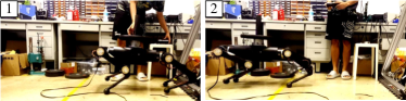
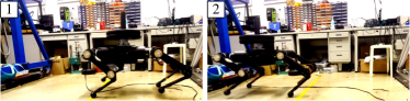
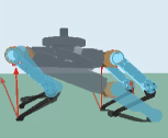
  We validate our controller in various simulations and real-world experiments on our quadruped robot Sirius-belt. The hardware tests showcase that the robot with the proposed control framework is able to trot forward stably while carrying a 20 kg un-modeled payload (84% of body weight) as shown in Fig. 1. Our method can not only reduce tracking errors but also the vibration amplitude of robot states under dynamic uncertainties.

In the context of Model Predictive Control (MPC) applied to quadruped robots, commonly the robot’s body is treated as a Single Rigid Body (SRB) and the state of the robot can be defined as follows:

$\displaystyle{\bm{x}}=[{\bm{\theta}}^{T}~{}{\bm{p}}^{T}~{}{\bm{\omega}}^{T}~{}{\bm{v}}^{T}~{}g]^{T}$

(1)

Where ${\bm{\theta}},{\bm{p}},{\bm{\omega}},{\bm{v}}\in\mathbb{R}^{3}$ are the Euler angles, positions, angle velocities, and linear velocities of robot body in the world frame, ${g}$ is the gravitational acceleration.

In each control cycle of the MPC algorithm, the future behavior of the robot is predicted using the floating base model, and its discrete-time formulation [1] is as follows:

$\displaystyle{\bm{x}_{t+1}}={A_{t}\bm{x}_{t}}+{B_{t}\bm{u}_{t}}$

(2)

Where ${\bm{x}_{t}}\in\mathbb{R}^{13}$ is the states of the robot at time step ${t}$, ${\bm{u}_{t}}\in\mathbb{R}^{12}$ are Ground React Forces (GRFs) which are inputs of the system at time step ${t}$, ${A_{t}}\in\mathbb{R}^{13\times 13}$ is the matrix related with states at time step ${t}$, and ${B_{t}\in\mathbb{R}^{13\times 12}}$ is the matrix about inputs at time step ${t}$.

The equation (2) is based on the model of the robot body after being linearized and simplified (ignoring the dynamic of legs). In real-world scenarios, practical robots inevitably exhibit deviations from this model as mentioned before.

The primary sensors commonly employed in quadruped robots are the inertial measurement unit (IMU) and encoders, which provide measurements of essential robot states, such as Euler angles and body height. These sensor measurements are reasonable approximations of the true values of these states. Consequently, our focus lies in constructing the error model based on these sensor data.

In this paper, An ARMAV error model fitted from sensor data is implemented in traditional MPC to compensate for errors of dynamics uncertainties. By using estimated GRFs as indicators to predict potential state errors, we modify the method to improve its performance in quadruped robot applications. The modified ARMAV($n,m$) error model has the following form (derived from the procedure outlined in Section III-B and III-C):

$\displaystyle\begin{split}&{\bm{e}_{t}}-{\Phi_{1}}{\bm{e}_{t-1}}-{\Phi_{2}}{\bm{e}_{t-2}}+...+{\Phi_{n}}{\bm{e}_{t-n}}=\\ &{\bm{a}_{t}}-{\Theta_{1}}{\bm{a}_{t-1}}-{\Theta_{2}}{\bm{a}_{t-2}}...-{\Theta_{m}}{\bm{a}_{t-m}}+{C_{t}}{\bm{u}_{t}}\end{split}$

(3)

Where ${\bm{e}_{t}}\in\mathbb{R}^{4}$ is the error of robot state at time step ${t}$, ${n}$ is autoregression (AR) parameters of the model, ${m}$ is the moving average (MA) parameters of the model, ${\Phi_{i}}$, ${\Theta_{i}}\in\mathbb{R}^{4\times 4}$ are the matrix about AR and MA model respectively, ${C_{t}}\in\mathbb{R}^{4\times 12}$ is the matrix related with inputs in the error model.

Based on the error model (3) and obtaining predicted values of future state errors which is illustrated in Section III-A, the robot states after compensation are expressed as follows:

$\displaystyle{\bm{\tilde{x}_{t+1}}}={\bm{x}_{t+1}}+{S}{\bm{\hat{e}_{t+1}}}$

(4)

Where ${S}\in\mathbb{R}^{13\times 4}$ is the select matrix for error model.

Quadruped robot locomotion entails the critical task of regulating the position and orientation of the robot’s body, commonly referred to as robot states, in accordance with the desired commands. Based on the future states of the robot, MPC outputs the suitable GRFs to attain the desired robot states via optimization. This quadratic programming problem can be formulated as below:

	$\displaystyle\min_{\bm{u}}\quad\quad\quad$	$\displaystyle\sum_{k=0}^{N-1}l({\bm{\tilde{x}_{t+k}}},{\bm{u_{t+k}}})$		(5a)
	$\displaystyle{s.t.}\quad\quad\quad$	$\displaystyle{\bm{\tilde{x}_{t+k+1}}}=A_{t}{\bm{x}_{t+k}}+B_{t}{\bm{u}_{t+k}}+{S}{\bm{\hat{e}_{t+k+1}}},$		(5b)
		$\displaystyle k=0,1,...,N-1$
		$\displaystyle{\bm{x}_{t}}=\bm{x}(t)$		(5c)
		$\displaystyle g_{k}({\bm{\tilde{x}_{t+k}}},{\bm{u_{t+k}}})=0,\quad k=0,1,...,N$		(5d)
		$\displaystyle h_{k}({\bm{\tilde{x}_{t+k}}},{\bm{u_{t+k}}})\geq 0,\quad k=0,1,...,N$		(5e)

Where ${T}$ is the predict horizon, $l(\cdot)$ is the stage quadratic cost function, ${\bm{x}_{t}}$ is the current state at time step $t$, ${\bm{x}_{t+k}}$ is the predicted state at time step $t+k$ based on linear body dynamic, $g_{k}(\cdot)$ and $h_{k}(\cdot)$ are general equality, inequality constraints respectively.

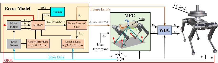
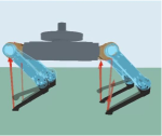
The overall control framework is illustrated in Fig. 2. The procedure is that the error model is derived from the error data collected in the sensors on the robot within every control cycle and the model uses historical data to predict future state errors. Subsequently, the Controller leverages these prognostic state errors to effectuate compensatory adjustments, countering discrepancies arising from the control model. The compensation strategy is twofold: 1. The error model employs a multi-step prediction approach to mitigate disparities within the MPC; 2. One step-ahead prediction is used to compensate for the Whole-body Control (WBC).

The ARMAV model[16] is a widely used statistical method for analyzing and predicting time series data. It has been successfully applied in various fields such as marketing prediction[17], manufacturing [18], resources management [19, 20], and so forth. One of its key strengths lies in its ability to capture and predict periodic behavior. Given that the locomotion of our quadruped robots exhibits periodic patterns, the ARMAV model is well-suited for error prediction in this context. The formulation of the ARMAV($n,m$) model is presented below:

	$\displaystyle{\bm{z}_{t}}-{\Phi_{1}}{\bm{z}_{t-1}}-{\Phi_{2}}{\bm{z}_{t-2}}-...-{\Phi_{n}}{\bm{z}_{t-n}}=$		(6)
	$\displaystyle{\bm{a}_{t}}-{\Theta_{1}}{\bm{a}_{t-1}}-{\Theta_{2}}{\bm{a}_{t-2}}-...-{\Theta_{m}}{\bm{a}_{t-m}}$

where ${\bm{z}_{t}}\in\mathbb{R}^{r}$ represents the data sample at time step ${t}$, ${\bm{a}_{t}}\in\mathbb{R}^{r}$ is the residual modeling noise at time step ${t}$, ${\Phi_{i}}\in\mathbb{R}^{r\times r}$ is the parameters matrix related with AR model and ${\Theta_{i}}\in\mathbb{R}^{r\times r}$ is the parameters matrix about MA model.

The update of ${\bm{a}_{t}}$ and one-step ahead prediction of ARMAV($n,m$) model can be obtained as the following equation:

	$\displaystyle{\bm{\hat{z}_{t+1}}}={E}[{\bm{z}_{t}}|t]={\Phi_{1}}{\bm{z}_{t}}+{\Phi_{2}}{\bm{z}_{t-1}}+...+{\Phi_{n}}{\bm{z}_{t-n+1}}$		(7)
	$\displaystyle-{\Theta_{1}}{\bm{a}_{t}}-{\Theta_{2}}{\bm{a}_{t-1}}-...-{\Theta_{m}}{\bm{a}_{t-m+1}}$

$\displaystyle{\bm{a}_{t+1}}={\bm{z}_{t+1}}-{\bm{\hat{z}_{t+1}}}$

(8)

Where ${\bm{\hat{z}_{t+1}}}$ is the predicted value for time step ${t+1}$.

As for k-step ahead prediction, it is derived from iteration which means that the next predicted values are based on the before predicted values as well as real data:

	$\displaystyle{\bm{\hat{z}_{t+k}}}$	$\displaystyle={\Phi_{1}}{\bm{\hat{z}_{t+k-1}}}+{\Phi_{2}}{\bm{\hat{z}_{t+k-2}}}+...+{\Phi_{n}}{\bm{z}_{t+k-n}}$		(9)
		$\displaystyle-{\Theta_{1}}{\bm{\hat{a}_{t+k-1}}}-{\Theta_{2}}{\bm{\hat{a}_{t+k-2}}}-...-{\Theta_{m}}{\bm{a}_{t+k-m}}$

$${\bm{\hat{a}_{t+l-m}}}=0,l=1,2,3,...,k$$

(10)

Due to the nonlinearity of the ARMAV($n,m$) model, parameter estimation is a non-linear problem. A viable solution is to obtain the initial guess values through the inverse function of ARMAV($n,m$):

$${\bm{a}_{t}}={\bm{z}_{t}}-{I_{1}}{\bm{z}_{t-1}}-{I_{2}}{\bm{z}_{t-2}}-...-{I_{l}}{\bm{z}_{t-l}}...$$

(11)

Where ${I_{l}}$ is the inverse coefficient.

In the inverse function form of the ARMAV model, the relations in ${\Phi_{i}}$ and ${\Theta_{i}}$ expressed by the inverse coefficients ${I_{j}}$ are linear for an arbitrary ARMAV($n,m$) model. Since coefficients ${I_{j}}$ are AR parameters of the infinite expansion of the ARMAV model, it can be estimated well by the Least-Squares (LS) approach.

Substituting for ${\bm{a}_{t}}$ from equation (11) in equation (6), the relation between ${\Phi_{i}}$, ${\Theta_{i}}$ and ${I_{j}}$ can be expressed as following:

$$\begin{split}&({E}-{\Phi_{1}}B-...{\Phi_{n}}B^{n}){\bm{z}_{t}}=\\ &({E}-{\Theta_{1}}B-...-{\Theta_{m}}B^{m})({E}-{I_{1}}B-{I_{2}}B^{2}-...){\bm{z}_{t}}\end{split}$$

(12)

Where ${E}$ is identity matrix and ${B}$ is back shift operator (for instance, ${B^{i}\bm{z}_{t}=\bm{z}_{t-i}}$).

Equating the coefficients of equal powers of $B$, the following is obtained:

$\displaystyle\begin{split}&{\Phi_{1}}={\Theta_{1}}+{I_{1}}\\ &{\Phi_{2}}={\Theta_{2}}-{\Theta_{1}}{I_{1}}+{I_{2}}\\ &{\Phi_{3}}={\Theta_{3}}-{\Theta_{1}}{I_{2}}-{\Theta_{2}}{I_{1}}+{I_{3}}\\ &.\ .\ .\\ &{\Phi_{j}}={\Theta_{j}}-{\Theta_{1}}{I_{j-1}}-{\Theta_{2}}{I_{j-2}}-...-{\Theta_{j-1}}{I_{1}}+{I_{j}}\end{split}$

(13)

Where it is assumed that ${\Theta_{j}}=0$ for ${j>m}$ and ${\Phi_{j}}=0$ for ${j>n}$.

According to equation (13), for ${j>\max(n,m)}$ the particular case of it can be derived:

$$({E}-{\Theta_{1}}B-{\Theta_{2}}B^{2}-...-{\Theta_{m}}B^{m}){I_{j}}=0$$

(14)

It is straightforward that once estimated values of inverse coefficients are known the initial values of AR parameters as well as MA parameters can be derived from equation (13) and (14). The initial guess of ${I_{j}}$ is given from pure AR($p$) model:

$${\bm{z}_{t}}={\Phi_{1}}{\bm{z}_{t-1}}+{\Phi_{2}}{\bm{z}_{t-2}}+...+{\Phi_{p}}{\bm{z}_{t-p}}+{\bm{a}_{t}}$$

(15)

Based on the estimates of ${I_{j}}$ in AR($p$) model, ${\Theta_{i}}$ is derived from equation (14). Then by substituting these ${\Theta_{i}}$ in equation (13), the explicit solution of ${\Phi_{i}}$ is got. Since the initial values of ${\Theta_{i}}$ are derived from equation (14) that requires ${j>\max(n,m)}$, for getting all the ${\Theta_{i}}$, it is reasonable to take the order of AR($p$) model as:

$$p=\max(n,m)+m$$

(16)

One of the reasons why the ARMAV model is so popular is that it is always possible to represent the dynamics of a stable stationary stochastic system with the ARMAV($n,m$) model, which means that only if the order of system $n$ and $m$ increases can the error of the model decrease into as small as we want. This flexibility allows for fitting the data to different orders of the ARMAV model based on the complexity of the system and the desired level of accuracy.

The reduced trend of residual sum of squares (RSS) is a good indicator to evaluate the adequacy of the model, when RSS drops significantly which means that the model may not be enough and the order of ARMAV($n,m$) should be increased. F checking criterion [16] is an indicator to evaluate the drop trend of RSS :

$\displaystyle F=\frac{A_{1}-A_{0}}{s}\div\frac{A_{0}}{N-r}\sim F(s,N-r)$

(17)

Where ${A_{0}}$ is the smaller RSS in the unrestricted model, ${A_{1}}$ is the larger RSS in the restricted model, ${s}$ is the number of restricted parameters, ${N}$ is the number of samples, ${r}$ is the number of estimated parameters, and ${F(s,N-r)}$ is F-distribution with ${s}$ and ${N-r}$ degrees of freedom. If ${F<F_{s,N-r}^{\alpha}}$, RSS can be regarded as drop significantly with confidence ${\alpha}$.

The procedure of the F-testing method based on equation (17) is used to choose the order of the ARMAV model. The first step is to determine the AR order $n$ by comparing the RSS of ARMAV($2k+2,2k+1$) and ARMAV($2k,2k-1$) starting from $k=1$. Then, the MA order $m$ is reduced to determine the desired value by a similar method. At last, the autocorrelation of residuals with lag $l$ should be confirmed:

$\displaystyle\rho_{l}=\frac{\sum_{t=1}^{N-l}a_{t}a_{t+l}}{N-l}\div\frac{\sum_{t=1}^{N}a_{t}a_{t}}{N}$

(18)

In this case, to assess the performance of the proposed controller when model parameters are inaccurate, two groups have been established: 1. the control model is perfect (ground truth case); 2. the mass of the model is set to 34.7 kg (the real mass of the robot is 23.7 kg).

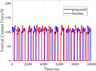
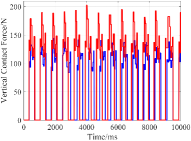
The locomotion performances of quadruped robots in two cases are compared based on the displacement of CoM and the GRFs in the vertical direction. The comparative outcomes are visually presented in Fig. 3 and Fig. 4.

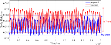
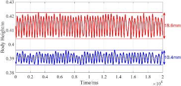
In the simulation, the robot’s desired body height is set to 0.38 m. Fig. 3 shows that the error model helps to bring the robot’s state closer to the desired value, and reduces the vibration amplitude of the body height for both cases. For the perfect model case, errors mostly arise from the model’s simplified and linearized process. Therefore, the error model only achieves a slight improvement of locomotion by reducing 21.7% vibration of CoM, from 8.7 mm to 6.9 mm. In the inaccurate mass case, there is an 11 kg gap in the mass parameter between the robot and the model. This is the reason why the body height vibrates largely. By adding the error model, this model inaccuracy is compensated and its CoM vertical vibration is decreased by 41.4%, from 18.6 mm to 10.9 mm. Fig. 4 shows that the error model helps MPC adjust the GRFs to achieve more suitable values for such improvement. In conclusion, the error model can improve the locomotion performance of the robot in both cases, and the improvement is more obvious under the inaccurate model parameter situation.

For the quadruped robot in the real world, transporting various payloads is one of its common applications. However, the parameters of payload such as mass are random depending on application scenarios and it is difficult to be included in the control model in advance. To simulate such a situation, in this part, an un-modeled payload is applied to the robot body.

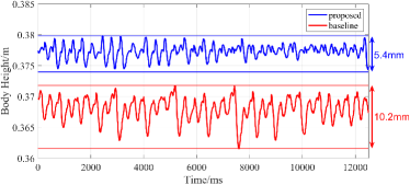
In the simulation, an 8 kg payload is exerted on the robot body, which is excluded from the control model. The vibration of body height under this situation is shown in Fig. 5(a). The baseline controller fails to restore the robot to the desired state, as the payload is not modeled, and the body height remains below the desired value of 0.38 m. On the other hand, the proposed controller has a noticeable effect in raising the body height to the desired value while simultaneously reducing the vibration by 47.1%. Additionally, as shown in Fig. 5(b) and Fig. 5(c), the performance of the robot with the baseline controller is less stable compared to the robot with the proposed controller and it falls down after 30 seconds of trotting. In conclusion, the proposed controller can make the robot attain the desired body height, reduce the vibration of CoM, and ensure stable trotting even under an unknown payload in the simulation.

The experiments are all implemented in our quadruped robot Sirius-Belt. Each leg of the robot consists of three degrees of freedom (DoFs) actuated by three electric motors. So Sirius-Belt has a total of 18 DoFs. The dimension (Length$\times$Width$\times$Height) of the robot is $0.78\times 0.37\times 0.54$ m (fully standing). The maximum torque for knee joint actuators (Gear Ratio: 9 to 1) and hip joint actuators (Gear Ratio: 6 to 1) are 38 Nm and 30 Nm respectively. The controller runs in an onboard Upboard (ATOM x5-Z8350).

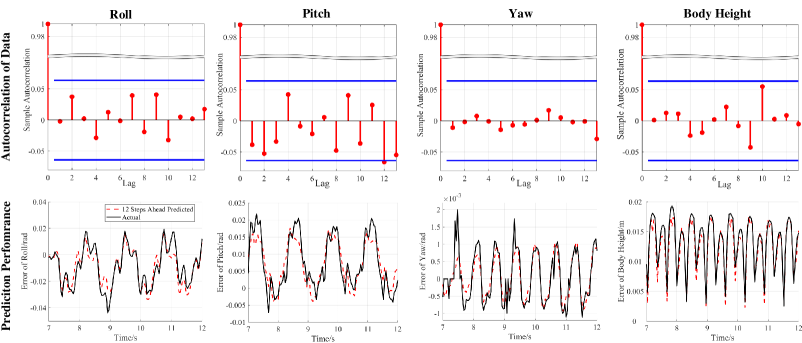
Real-world data are collected from the actual robotic system during trotting. By equation (18), the residuals autocorrelation of Euler angles and body height in the error model is depicted in the up part of Fig. 6. It can be seen that the autocorrelation of residuals between different times are all within the boundary of ${-\frac{2}{\sqrt{N}}}$ and ${\frac{2}{\sqrt{N}}}$ (blue lines in Fig. 6), which can prove that residuals in error model can be regarded as uncorrelated data with mean zero and variance ${N^{-1}}$. The below part of Fig. 6 shows 12 (which is our MPC predicted horizon) steps ahead of predicted values from the error model in Euler angles and body height which are very close to the true values of the real-world robot.

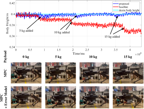
In the first hardware experiment, the payload from 5 kg to 15 kg is added on the Sirius-Belt during trotting in place one by one. Concurrently, the data of real robot states in the baseline controller and proposed controller are recorded to evaluate their performance. The body height of the robot during the experiment is shown in Fig. 7.

Table. I shows the performance of the proposed controller and baseline in the real-world experiment by Mean Absolute Error (MAE) and Mean Squared Error (MSE). It reveals that the proposed controller exhibits improved state tracking performance for roll, pitch, and body height in comparison to the baseline controller. However, it indicates that no significant effect is observed in the yaw state due to its pretty small errors.

The second experiment is to evaluate the performance of the proposed controller in the robot’s forward trotting. The results shown in Fig. 1 prove that the proposed controller enables the Sirius-Belt carrying a 20 kg un-modeled payload to achieve a stable forward trotting, where the mean of CoM height is 0.397 m (the desired value is 0.4 m) with standard deviation (STD) of 0.0011 m. However, the counterpart with the baseline controller is unstable even in a 10 kg payload (mean = 0.369 m and STD = 0.0035 m).

The obtained results validate the effectiveness of the proposed controller in facilitating stable trotting for the robot, even when confronted with un-modeled payloads. Notably, the robot with the proposed controller consistently maintains the desired body height throughout the experiments. This capability proves advantageous when the robot is tasked with carrying heavy loads, as it prevents excessive strain on the knee actuators.

References

- [1] Di Carlo, Jared, et al. ”Dynamic locomotion in the MIT cheetah 3 through convex model-predictive control.” 2018 IEEE/RSJ international conference on intelligent robots and systems (IROS). IEEE, 2018.
- [2] Kim, Donghyun, et al. ”Highly dynamic quadruped locomotion via whole-body impulse control and model predictive control.” arXiv preprint arXiv:1909.06586 (2019).
- [3] Song, Zhitao, et al. ”An Optimal Motion Planning Framework for Quadruped Jumping.” 2022 IEEE/RSJ International Conference on Intelligent Robots and Systems (IROS). IEEE, 2022.
- [4] Feng, Gilbert, et al. ”Genloco: Generalized locomotion controllers for quadrupedal robots.” Conference on Robot Learning. PMLR, 2023.
- [5] Neunert, Michael, et al. ”Whole-body nonlinear model predictive control through contacts for quadrupeds.” IEEE Robotics and Automation Letters 3.3 (2018): 1458-1465.
- [6] Meduri, Avadesh, et al. ”Biconmp: A nonlinear model predictive control framework for whole body motion planning.” IEEE Transactions on Robotics 39.2 (2023): 905-922.
- [7] Tournois, Guido, et al. ”Online payload identification for quadruped robots.” 2017 IEEE/RSJ International Conference on Intelligent Robots and Systems (IROS). IEEE, 2017.
- [8] Minniti, Maria Vittoria, et al. ”Adaptive CLF-MPC with application to quadrupedal robots.” IEEE Robotics and Automation Letters 7.1 (2021): 565-572.
- [9] Sombolestan, Mohsen, Yiyu Chen, and Quan Nguyen. ”Adaptive force-based control for legged robots.” 2021 IEEE/RSJ International Conference on Intelligent Robots and Systems (IROS). IEEE, 2021.
- [10] Pandala, Abhishek, et al. ”Robust predictive control for quadrupedal locomotion: Learning to close the gap between reduced-and full-order models.” IEEE Robotics and Automation Letters 7.3 (2022): 6622-6629.
- [11] Sun, Yu, et al. ”Online learning of unknown dynamics for model-based controllers in legged locomotion.” IEEE Robotics and Automation Letters 6.4 (2021): 8442-8449.
- [12] Yang, Wen-Shan, Wei-Chun Lu, and Pei-Chun Lin. ”Legged robot running using a physics-data hybrid motion template.” IEEE Transactions on Robotics 37.5 (2021): 1680-1695.
- [13] Fawcett, Randall T., et al. ”Toward a data-driven template model for quadrupedal locomotion.” IEEE Robotics and Automation Letters 7.3 (2022): 7636-7643.
- [14] Chang, Alexander H., et al. ”Learning to jump in granular media: Unifying optimal control synthesis with Gaussian process-based regression.” 2017 IEEE International Conference on Robotics and Automation (ICRA). IEEE, 2017.
- [15] Torrente, Guillem, et al. ”Data-driven MPC for quadrotors.” IEEE Robotics and Automation Letters 6.2 (2021): 3769-3776.
- [16] Pandit, Sudhakar Madhavrao, Shien‐Ming Wu, and Talivaldis I. Šmits. ”Time Series and System Analysis with Applications by Sudhakar Madhavrao Pandit and Shien‐Ming Wu.” (1984): 1924-1925.
- [17] Xu, Weijun, et al. ”Forecasting energy consumption using a new GM–ARMA model based on HP filter: The case of Guangdong Province of China.” Economic Modelling 45 (2015): 127-135.
- [18] Aghdam, B. H., M. Vahdati, and M. H. Sadeghi. ”Vibration-based estimation of tool major flank wear in a turning process using ARMA models.” The International Journal of Advanced Manufacturing Technology 76 (2015): 1631-1642.
- [19] Shafaei, Maryam, and Ozgur Kisi. ”Lake level forecasting using wavelet-SVR, wavelet-ANFIS and wavelet-ARMA conjunction models.” Water Resources Management 30 (2016): 79-97.
- [20] Erdem, Ergin, and Jing Shi. ”ARMA based approaches for forecasting the tuple of wind speed and direction.” Applied Energy 88.4 (2011): 1405-1414.
- [21] Di Carlo, Jared. Software and control design for the MIT Cheetah quadruped robots. Diss. Massachusetts Institute of Technology, 2020.