Adaptive Real-Time Grid Operation via Online Feedback Optimization with Sensitivity Estimation
Abstract
In this paper we propose an approach based on an Online Feedback Optimization (OFO) controller with grid input-output sensitivity estimation for real-time grid operation, e.g., at subsecond time scales. The OFO controller uses grid measurements as feedback to update the value of the controllable elements in the grid, and track the solution of a time-varying AC Optimal Power Flow (AC-OPF). Instead of relying on a full grid model, e.g., grid admittance matrix, OFO only requires the steady-state sensitivity relating a change in the controllable inputs, e.g., power injections set-points, to a change in the measured outputs, e.g., voltage magnitudes. Since an inaccurate sensitivity may lead to a model-mismatch and jeopardize the performance, we propose a recursive least-squares estimation that enables OFO to learn the sensitivity from measurements during real-time operation, turning OFO into a model-free approach. We analytically certify the convergence of the proposed OFO with sensitivity estimation, and validate its performance on a simulation using the IEEE 123-bus test feeder, and comparing it against a state-of-the-art OFO with constant sensitivity.
Index Terms:
Online Feedback Optimization, Real-time AC Optimal Power Flow, Recursive Estimation, Voltage Regulation1 These two authors contributed equally.
Funding by the Swiss Federal Office of Energy through the projects “ReMaP” (SI/501810-01) and “UNICORN” (SI/501708), the Swiss National Science Foundation through the NCCR Automation, and by the ETH Foundation is gratefully
acknowledged.
I Introduction
The increasing amount of controllable, yet sometimes unpredictable, power resources in electrical grids, e.g., renewable generation, electric vehicles, flexible loads, etc., leads to new challenges and opportunities in the operation of power systems. On the one hand, these new controllable elements allow to minimize the grid operational cost and promote a transition to a more sustainable power system. On the other hand, given the volatility and unpredictability of these resources, fast control decisions are required to avoid constraint violations, e.g., overvoltages. This is especially relevant in distribution grids, where many of these resources are deployed. However, measurement scarcity and poor grid models challenge grid operation at such low voltage levels.
One way to leverage the controllability of these resources and to optimize the grid operation is by solving an AC Optimal Power Flow (AC-OPF) [1], an optimization problem to determine the set-points of controllable resources that minimize the operational cost and enforce grid safety requirements, e.g., voltage limits, line thermal limits, etc. Unfortunately, standard AC-OPF requires a) full grid observability, e.g., measurements of all active and reactive power injections and consumptions, and b) an accurate nonlinear grid model, e.g., its admittance matrix [1]. Yet, learning the model may require an extensive deployment of measurements across the network [2, 3], usually not available or affordable on the distribution system level. Furthermore, the volatility of renewable energy sources and household loads requires high sampling and control-loop rates to satisfy the grid constraints. Yet, solving a computationally expensive AC-OPF may pose a limit on these rates.
Online Feedback Optimization (OFO) [4, 5, 6] is a novel computationally efficient approach that allows to track the solutions of an AC-OPF problem under time-varying conditions using subsecond control-loop rates. OFO is based on a controller that uses grid measurements as feedback to iteratively steer the controllable input set-points towards the AC-OPF solutions, and has already been successfully tested in both simulations and experimental settings [7]. Furthermore, OFO neither requires full grid observability [8], nor an accurate nonlinear grid model. It only needs measurements of the outputs that need to be controlled, and the input-output sensitivity that matches a change in the input to a change in the output. This sensitivity is essentially a derivative of the power flow equations at the operating point [9], and thus depends on the grid state and exogenous disturbances, e.g., loads. Hence, constructing an accurate sensitivity requires the grid model and full measurements of the grid to evaluate it. To avoid these requirements, some OFO approaches use a constant approximate linear model, and thus a constant approximate sensitivity [6, 8, 7]. Even though OFO is robust against small approximation errors in this sensitivity [7], an inaccurate sensitivity introduces a model-mismatch that may lower the approach performance [10]. Therefore, some model-free approaches try to operate the system optimally without requiring a model or sensitivity. First, reinforcement learning allows to disregard the model, and instead take decisions based solely on measurements [11]. However, reinforcement learning has limited theoretical guarantees, and may not be able to enforce the grid safety constraints during its learning phase. Second, data-driven control [12, 13, 14] based on Willems Fundamental lemma [15] allows to compute the sensitivity after gathering sufficient data. Yet, these approaches estimate a constant linear model, and thus may fail to adapt to different operating points. Finally, zeroth-order gradient-free methods as [16] allow to operate the system while continuously estimating and updating the sensitivity. However, [16] requires a sufficient time-scale separation between the sensitivity estimation procedure and the feedback optimization, which may lower the convergence rate of the entire approach if the measurement sample rate is restricted due to communication limits.
Therefore, in this paper, with a similar spirit as in the extremum seeking approach [16], we propose a model-free OFO approach that sequentially estimates a time-varying sensitivity while operating the grid, bypassing the need to know the whole grid model accurately, and to have full grid observability. Our contributions are as follows: First, we design a sensitivity learning approach via recursive least squares [17, 18]. We use as measurements the change in the outputs caused by a change of the controllable inputs. Second, we combine this sensitivity estimation with a persistently exciting OFO that gathers enough information about the sensitivity while driving the control inputs towards the AC-OPF solutions. Third, we certify the convergence of both the estimated sensitivity and the control input towards the true sensitivity and the time-varying solution of the AC-OPF, respectively. Fourth and finally, we simulate the proposed OFO controller with sensitivity estimation on the 3-phase, unbalanced IEEE 123-bus test feeder [19] using real consumption data, and show its superior performance over a state-of-the-art OFO with a constant sensitivity approximation.
The paper is structured as follows: Section II presents some preliminaries on grid models, AC-OPF and OFO. Section III explains our proposed OFO with sensitivity estimation approach, and provides theoretical convergence guarantees. Section IV shows the simulation on a test feeder. Finally, Section V concludes and discusses further work.
II Preliminaries: Grid Model, AC-OPF and OFO
II-A Grid Model
For each bus of a -bus power system we define the voltage magnitude as , the active and reactive power as and , respectively. We obtain the vectors , , and of dimension by stacking the individual bus quantities, i.e., . We define the control input vector consisting of all the controllable resources (e.g. active and reactive generation and flexible loads in and , slack bus voltage magnitude through tap changers); the output vector (e.g. voltage magnitude elements in ) with all the quantities that we measure and want to control through the inputs; and the disturbance vector with all uncontrollable power injections (e.g. conventional consumption loads in and ). The grid admittance matrix and the power flow equations allow to define an input-output map that characterizes the output as a non-linear function of and :
| (1) |
The input-output map is not typically available in closed form, since in general it is not possible to derive an analytical expression of (in ) as a function of and (in and ) using the power flow equations [1]. Yet, the local existence of a continuous differentiable map can be guaranteed by the implicit function theorem [20].
II-B AC Optimal Power Flow for Grid Operation
The operation of a power grid consists of deciding the input at each time instant . An AC-OPF allows to formulate this decision process as an optimization problem:
| (2) | ||||
where is the operational cost on the input ; is a penalty function to enforce some grid specification on the output , e.g., voltage limits; is the time-varying set of admissible inputs that defines the operational constraints on , e.g., power limits ; and is the disturbance value at time , e.g., uncontrollable loads or non-dispatchable generation. The nonlinear input-output model (1) in (2) relates the outputs to the chosen input.
Optimal real-time decision making consists of first taking measurements ; then, solving the AC-OPF problem (2), and finally applying the solution to the system. Then, this is repeated at the next time step .
II-C Linear Power Flow Approximation
Solving AC-OPF problems (2) to determine the set-points of power resources is a compelling and valuable tool for grid operators, but it comes with some drawbacks: First, the full nonlinear model of the grid is needed. Second, solving the AC-OPF (2) can be computationally expensive, which may jeopardize its use for real-time grid operation. This can be circumvented by linearizing the map in (1) at an operating point [21, 22, 1], e.g., the zero-injection point , to obtain the approximation
| (3) | ||||
where is an offset representing the output value when , e.g., p.u. for all voltage magnitudes. The matrices and are evaluated at the operating point, and represent the sensitivities of the output with respect to changes in the input and disturbance , respectively. This linear approximation (3) can substitute the nonlinear map in the AC-OPF (2) to get
| (4) | ||||
II-D Online Feedback Optimization (OFO)
Solving the AC-OPF with linear power flow approximation (4) is computationally efficient and could be employed in real-time operation. However, this approach does not take advantage of output measurements , since it only feeds through the inaccurate linear model (3). Hence, such a feedforward approach introduces a model-mismatch that can cause a performance degradation, and even lead to constraint violations, e.g., under and overvoltages.
Instead, OFO is a novel approach [5, 6, 4] that uses as feedback to achieve a safer grid operation and track the solution of the AC-OPF (2) under time-varying conditions. For that, OFO turns a standard optimization algorithm, in our case projected gradient decent [23], into a feedback controller that takes the grid output measurements , instead of computing the output via the grid model (1) or the linearized one (3). Projected gradient decent consists of a gradient step and a projection: First, we compute the gradient of the cost function in (4):
To minimize the operational cost, the current input is pushed along the direction of the negative gradient with a step size , and then it is projected onto the feasible space to enforce the operational constraints on the input, i.e.,
| (5) | ||||
where is the projection of onto , which is typically easy to evaluate for power grid operation [6], especially if is a box constraint.
III Online Feedback Optimization with Sensitivity Estimation
The OFO controllers are robust, i.e., preserve stability, against using a constant power flow sensitivity approximation instead of the actual one [7, 10]. Unfortunately, even if the overall system is stable, a model mismatch between and may lead to a difference between the solution of the AC-OPF problem and the values produced by the OFO controller (5) [10]. Therefore, we propose an approach to sequentially update the sensitivity into a good approximation of the true sensitivity , and thus avoid a potential performance degradation. For that, we will consider the sensitivity as a time-varying parameter , and propose a recursive least-squares approach to generate sensitivity estimates using the measured variations of and over time, and respectively. Then, in every time step we feed this estimated sensitivity to the OFO as in Figure 1.
III-A Sensitivity Estimation
Due to the non-linearity of , the true sensitivity depends on the values of and . The temporal variation of the disturbance and the input , e.g., due to applying the OFO controller (5) in the input case, produces a time-varying sensitivity . Instead of learning the dependency on and , we model a time-varying sensitivity with the following random process:
| (6) | ||||
where is the column-wise vector representation of the sensitivity matrix , denotes a change of the input , and is a Gaussian process noise with covariance , that represents how the sensitivity changes over time. We make the part of the process noise proportional to , since a large can trigger a larger change in the true sensitivity that depends on , and the part independent of to account for a uncontrolled random change that can affect the sensitivity as well.
Next, to derive a measurement equation for the sensitivity , consider the first-order Taylor approximation of
| (7) | ||||
At each time , we measure , and compute the variation . Based on the Taylor approximation (7), we treat this variation as a noisy linear measurement of through a measurement model that depends on :
| (8) | ||||
where , with the Kronecker product , and is a Gaussian measurement noise with covariance . Again, the part independent of in the measurement noise represents the effect of an uncontrolled random disturbance change , while the other parts and encapsulate the second-order error of the Taylor approximation (7).
To update the sensitivity estimate , we combine the information given by the previous sensitivity estimate , and the measurements (8). We compute the new sensitivity estimate through a Bayesian update represented in the following least-squares problem [17, 18]:
where is the covariance matrix representing the uncertainty of the sensitivity estimate , and is the norm of with respect to a positive definite matrix . The resulting recursive estimation can be expressed as a Kalman filter [24]:
| (9) | ||||
where is the identity matrix, and is the Kalman gain, which is well defined for an invertible , see later Assumption 1.
Remark 1
Note that for a diagonal measurement noise covariance , in the limit , the gain is , thus the sensitivity is not updated, and we keep the initial sensitivity, i.e., . Similarly, a large diminishes , and helps to tune how fast we want to learn or differ from the initial sensitivity. On the other hand, the process noise covariance represents our trust in our current model, and it also helps to tune the learning rate.
III-B Persistently Exciting OFO
To learn the time-varying sensitivity , we need to capture enough information via the measurement equation (8), i.e, we need to use different to explore different reactions and infer different elements of from them. This can be formalized via the persistency of excitation condition [25]: is persistently exciting if there exists a time span , such that for all , the matrix formed by columns for has full rank, i.e., . To achieve persistency of excitation, we perturb the OFO step (5) with , a bounded zero-mean white noise with independent and identically distributed elements with standard deviation , e.g., a truncated Gaussian distribution. As a result, we obtain the following persistently exciting OFO with estimated sensitivity :
| (10) | ||||
The resulting interconnected OFO, sensitivity learning and power grid is represented in the block diagram in Figure 1. At each time , a complete loop of the online optimization with sensitivity estimation can be represented as:
Remark 2
The sensitivity learning approach (9) is independent of the method used to update the input , since it only requires the increment and the measured . Hence, it is not only compatible with the projected-gradient-based OFO in (10), but can be combined with linearly simplified AC-OPF as (4), or other OFO approaches, e.g., primal-dual methods [6, 7], quadratic programming [26, 27], which may have other desirable properties, like strict constraint satisfaction or a faster convergence.
III-C Convergence Analysis
In this section we analyze the convergence of the estimated sensitivity produced by the sensitivity learning (9), and the input produced by the OFO (10), towards the true sensitivity and the solution of the AC-OPF (2), respectively. We certify this convergence assuming that the true sensitivity behaves according to the simplified dynamic process (6) and satisfies the linear measurements equation (8); and that the projected gradient descent used in (10) is a strongly monotone and Lipschitz continuous operator:
Definition 1 (Monotone and Lipschitz operator)
An operator is -strongly monotone if for all , and -Lipschitz continuous if .
Assumption 1
The functions and in (2) are continuously differentiable. The sensitivity satisfies (6) and (8) with independent and . Furthermore, for all , have a positive lower and upper bound, i.e., there exists such that , ; there exists such that ; and the operator in (10) is -strongly monotone and -Lipschitz continuous.
The continuous differentiability of and is common for typical cost functions in power systems, e.g., linear or quadratic , and quadratic penalty functions like . For strongly convex and Lipschitz smooth cost functions , the strong monotonicity and Lipschitz continuity of the gradient operator holds in certain regions around nominal operating points [10]. In particular, it would hold if using a usual linear approximation for the input-output map (1) [8]. Since and are restricted by the grid physical limits, e.g., power ratings, the upper bound of and are justified, since is differentiable in a compact set. The persistency of excitation ensures that with high probability. Then, if at least one and one for some . Finally, even though the true sensitivity is state dependent, i.e., , the process and measurement noises in (6) and (8) allow to overapproximate the actual behavior of the sensitivity via these simplifications. In conclusion, Assumption 1 is reasonable. Then, with a persistently exciting as in (10), we have the following convergence result:
Proposition 1
Under Assumption 1, and the persistently excited OFO updates (10), the sensitivity estimates (9) satisfy:
| (11) | ||||
where denotes the expectation, are positive constants, and the limit as goes to infinity. Furthermore, if the step size in (10) satisfies , so that , then we have
| (12) | ||||
Proof:
See Appendix. ∎
Proposition 1 establishes first that the estimated sensitivity converges in expectation to the true sensitivity with a bounded covariance. Additionally, the control input converges to the AC-OPF solution from (2) with a quantifiable tracking error determined by the bound of the sensitivity estimation covariance, the variance of the persistency of excitation noise , and the temporal variation of the AC-OPF solution , where can also be bounded by the temporal variation of and in the AC-OPF (2) [28].
IV Test Case
In this section we validate the proposed OFO with sensitivity estimation. We simulate a benchmark distribution grid under time-varying conditions during a 1-hour simulation with 1-second resolution, hence a 1 second control-loop rate. In particular, we show its superior performance against an OFO approach with a constant sensitivity. First we explain the simulation setup, and then we comment the results obtained.
IV-A Simulation Setup
- •
-
•
Disturbance : We consider uncontrollable active and reactive loads in our disturbance vector . To generate these load profiles we use -second resolution data of the ECO data set [29], then aggregate households and rescale them to the base loads of the 123-bus feeder. This gives us values of for every second during simulation time of 1h.
-
•
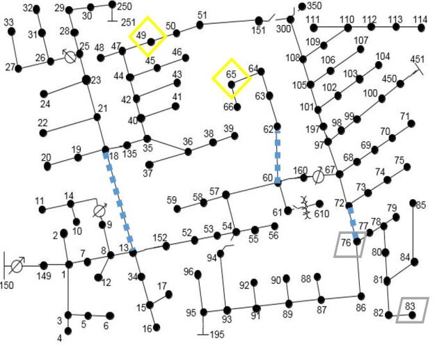
Controllable input set-points : We add two solar PV systems and two wind turbines to the grid as in [8], see Figure 2. They can inject active power, and inject and absorb reactive power on all three phases, which gives us 24 control inputs. We consider a slack bus 150 in Figure 2, with a controllable voltage magnitude through, e.g., a tap changer, which makes in total . The solar and wind generation profiles are generated based on a -minute solar irradiation profile [30] and a -minute wind speed profile [31]. Generation is assumed constant between samples. We use these profiles to set the time-varying upper limit of the feasible set , set the lower limit of active generation to , and define .
-
•
Output : We consider as output the voltage magnitudes of all phases at all buses except the slack bus, given that it is a control input.
-
•
AC-OPF cost function in (2): We use a quadratic cost that penalizes deviating from a reference: . The reference for the voltage magnitude at the slack bus is p.u. The reference for the controllable generation is the maximum installed power to promote using as much renewable energy as possible. The reference for reactive power is . Note that the cost function is continuously differentiable, and has a strongly monotone and Lipschitz continuous gradient as required in Assumption 1. We consider the voltage limits for all nodes as in [5, 8], and use the penalty function , with a sufficiently large penalization parameter to discourage violations. Again, this function is continuously differentiable, and has a monotone and Lipschitz continuous gradient.
- •
-
•
Persistency of excitation: We use a symmetric truncated Gaussian distribution with p.u. to introduce a low persistency of excitation noise that facilitates our sensitivity learning, but avoids introducing a big deviation in the input convergence, see (12).
-
•
Initializing sensitivity and linear model (3): We use the zero-injection operating point to initialize the sensitivity estimation, i.e., , see (3). In the first simulation (1: true admittance) we use the true admittance to compute , in the second (2: perturbed admittance) we use a perturbed admittance matrix, where we have introduce an up to error in the admittance of the lines indicated in Figure 2.
IV-B Results
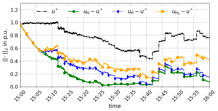
We analyze the simulation performance of OFO with sensitivity learning (9) and (10), and compare it against an OFO with constant sensitivity (5). We validate both results in Proposition 1: First, the estimated sensitivity converges to the real time-varying sensitivity . Second, the input converges to the AC-OPF solution (2).
IV-B1 True admittance
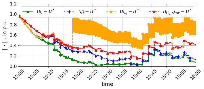
First we perform a simulation where we use the true admittance to derive the initial sensitivity in the linear power flow approximation (3). Figure 3 shows the norm of the AC-OPF solution of (2) that we calculate with the correct non-linear model and the disturbances . This optimal input is time-varying due to the changing solar radiation and wind speed in the limits , and the temporal variation of the loads in . Figure 3 shows how the OFO control input converges towards the optimal input using different sensitivities: The inputs produced by the OFO controller (5) with the exact sensitivity succeed in tracking the AC-OPF solution , with relatively small differences caused by the time-varying disturbances and/or available energy . However, when using the constant sensitivity in (5), there is a large difference between the generated control input and the optimal one . This gap is closed when using the OFO with sensitivity estimation (10), i.e., is able to converge to the AC-OPF solution of (2) with a small tracking error, as predicted by Proposition 1.
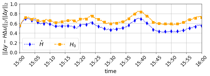
Figure 4 shows the relative error of the measurement equation (8). This helps to understand why OFO with sensitivity learning (9) performs better than with a constant sensitivity : The linearization error with estimated sensitivity gets lower respect to the one with . This means that the learned sensitivity becomes a more accurate linear approximation than (3), which causes the lower optimization error observed in Figure 3. Even though the error does not converge to when using , the sensitivity estimation approach (9) learns enough to drive the control set-points to the optimum, see Figure 3, which is our ultimate objective.
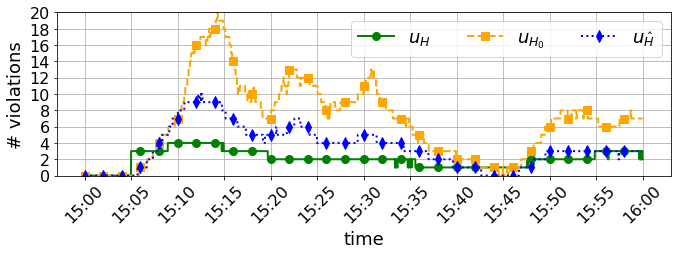
Finally, Figure 5 shows that the inputs , produced by the OFO with sensitivity estimation (10) result into much less voltage violations than from the OFO with constant sensitivity (5). Actually, the number of voltage violations of gets close to those of the OFO with true sensitivity . Hence, the OFO with sensitivity estimation not only reduces the distance to the AC-OPF solution, see Figure 3, but performs a better voltage regulation.
IV-B2 Perturbed admittance
In Figure 6 we show a simulation for which we perturb the admittance of the lines indicated in Figure 2 with an up to error. We observe how the OFO with sensitivity learning (10) is still able to track the AC-OPF solution of (2) in time-varying conditions. The OFO with a fixed sensitivity (5) and the same step size as diverges, since it tries to regulate the voltage with a wrong sensitivity that is too far from the actual one. Convergence is recovered with a lower step size in , but it still performs poorly at tracking the AC-OPF solution. This experiment allows us to conclude that the OFO with sensitivity estimation (10) is a model-free approach that does not require an accurate model, but learns it online.
V Conclusion and Outlook
Standard Online Feedback Optimization (OFO) typically uses an approximate input-output sensitivity, which may lower its performance. Alternative, one can compute the actual sensitivity, but that requires, having an accurate grid model and full grid observability, which is usually not available. In this work we have proposed a recursive estimation approach that provides Online Feedback Optimization (OFO) with a tool to learn the model sensitivity without extensive measurements, and thus improves its performance and turns OFO into a model-free approach. We have provided convergence guarantees when approximating the time-varying sensitivity behavior by a random process with linear measurements. We have established that even under time-varying conditions the estimated sensitivity and the control input converge to a neighborhood of the true sensitivity and the solution of the AC-OPF, respectively. Finally, we have validated with simulations using the IEEE 123-bus test feeder that our proposed OFO controller with sensitivity estimation performs successfully even though the actual sensitivity is state-dependent, i.e., it is able to track a time-varying optimal input while satisfying the grid specifications. In short, the proposed OFO controller with sensitivity estimation can be used as a model-free plug-and-play controller for real-time power grid operation that enables safe and optimal control.
An interesting future addition would be to investigate a more suitable way to design the persistency of excitation, possibly linked to the optimization problem, so that it explores specific directions of interest. Additionally, it would be interesting to observe how the proposed sensitivity estimation approach performs under a sudden change of topology caused by, e.g., a line fault, network split, etc.; under communication problems, e.g., delays, missing packages, recurrent outliers due to, for example, sensor misscalibration.
References
- [1] D. K. Molzahn and I. A. Hiskens, “A Survey of Relaxations and Approximations of the Power Flow Equations,” Foundations and Trends in Electric Energy Systems, vol. 4, no. 1-2, pp. 1–221, February 2019.
- [2] S. Bolognani, N. Bof, D. Michelotti, R. Muraro, and L. Schenato, “Identification of power distribution network topology via voltage correlation analysis,” in 52nd Conf. on Decision and Control, 2013, pp. 1659–1664.
- [3] K. Moffat, M. Bariya, and A. Von Meier, “Unsupervised impedance and topology estimation of distribution networks—limitations and tools,” IEEE Trans. Smart Grid, vol. 11, no. 1, pp. 846–856, 2020.
- [4] D. K. Molzahn, F. Dörfler, H. Sandberg, S. H. Low, S. Chakrabarti, R. Baldick, and J. Lavaei, “A survey of distributed optimization and control algorithms for electric power systems,” IEEE Trans. Smart Grid, vol. 8, no. 6, pp. 2941–2962, Nov. 2017.
- [5] A. Hauswirth, A. Zanardi, S. Bolognani, F. Dörfler, and G. Hug, “Online optimization in closed loop on the power flow manifold,” in 2017 IEEE Manchester PowerTech. IEEE, 2017, pp. 1–6.
- [6] E. Dall’Anese and A. Simonetto, “Optimal power flow pursuit,” IEEE Trans. Smart Grid, vol. 9, no. 2, pp. 942–952, Mar. 2018.
- [7] L. Ortmann, A. Hauswirth, I. Caduff, F. Dörfler, and S. Bolognani, “Experimental validation of feedback optimization in power distribution grids,” Electric Power Systems Research, vol. 189, p. 106782, 2020.
- [8] M. Picallo, S. Bolognani, and F. Dörfler, “Closing the loop: Dynamic state estimation and feedback optimization of power grids,” Electric Power Systems Research, vol. 189, p. 106753, 2020.
- [9] S. Bolognani and F. Dörfler, “Fast power system analysis via implicit linearization of the power flow manifold,” in 53rd Annual Allerton Conf. on Communication, Control, and Computing. IEEE, 2015, pp. 402–409.
- [10] M. Colombino, J. W. Simpson-Porco, and A. Bernstein, “Towards robustness guarantees for feedback-based optimization,” in 2019 IEEE 58th Conf. on Decision and Control. IEEE, 2019, pp. 6207–6214.
- [11] X. Chen, G. Qu, Y. Tang, S. Low, and N. Li, “Reinforcement learning for decision-making and control in power systems: Tutorial, review, and vision,” arXiv preprint arXiv:2102.01168, 2021.
- [12] J. Coulson, J. Lygeros, and F. Dörfler, “Data-enabled predictive control: In the shallows of the deepc,” in 2019 18th European Control Conference (ECC). IEEE, 2019, pp. 307–312.
- [13] C. Mugnier, K. Christakou, J. Jaton, M. De Vivo, M. Carpita, and M. Paolone, “Model-less/measurement-based computation of voltage sensitivities in unbalanced electrical distribution networks,” in 2016 Power Systems Computation Conference (PSCC). IEEE, 2016, pp. 1–7.
- [14] G. Bianchin, M. Vaquero, J. Cortes, and E. Dall’Anese, “Data-driven synthesis of optimization-based controllers for regulation of unknown linear systems,” Dec. 2021.
- [15] J. C. Willems, P. Rapisarda, I. Markovsky, and B. L. De Moor, “A note on persistency of excitation,” Systems & Control Letters, vol. 54, no. 4, pp. 325–329, 2005.
- [16] X. Chen, J. I. Poveda, and N. Li, “Model-free optimal voltage control via continuous-time zeroth-order methods,” Dec. 2021.
- [17] L. Lennart, “System identification: theory for the user,” PTR Prentice Hall, Upper Saddle River, NJ, vol. 28, 1999.
- [18] R. Isermann and M. Münchhof, Identification of dynamic systems: an introduction with applications. Springer Science & Business Media, 2010.
- [19] W. Kersting, “Radial distribution test feeders,” IEEE Trans. Power Syst., vol. 6, no. 3, pp. 975–985, 1991.
- [20] S. G. Krantz and H. R. Parks, The implicit function theorem: history, theory, and applications. Springer Science & Business Media, 2012.
- [21] S. H. Low, “Convex relaxation of optimal power flow—part i: Formulations and equivalence,” IEEE Transactions on Control of Network Systems, vol. 1, no. 1, pp. 15–27, 2014.
- [22] S. Bolognani and S. Zampieri, “On the existence and linear approximation of the power flow solution in power distribution networks,” IEEE Transactions on Power Systems, vol. 31, no. 1, pp. 163–172, 2015.
- [23] D. P. Bertsekas, “Nonlinear programming,” Journal of the Operational Research Society, vol. 48, no. 3, pp. 334–334, 1997.
- [24] A. H. Jazwinski, “Mathematics in science and engineering,” Stochastic processes and filtering theory, vol. 64, 1970.
- [25] E. Bai and S. Sastry, “Persistency of excitation, sufficient richness and parameter convergence in discrete time adaptive control,” Systems & Control Letters, vol. 6, no. 3, pp. 153–163, 1985.
- [26] V. Häberle, A. Hauswirth, L. Ortmann, S. Bolognani, and F. Dörfler, “Non-convex feedback optimization with input and output constraints,” IEEE Control Systems Letters, vol. 5, no. 1, pp. 343–348, 2020.
- [27] M. Picallo, D. Liao-McPherson, S. Bolognani, and F. Dörfler, “Cross-layer design for real-time grid operation: Estimation, optimization and power flow,” arXiv preprint arXiv:2109.13842, 2021.
- [28] I. Subotic, A. Hauswirth, and F. Dorfler, “Quantitative sensitivity bounds for nonlinear programming and time-varying optimization,” IEEE Transactions on Automatic Control, 2021.
- [29] C. Beckel, W. Kleiminger, R. Cicchetti, T. Staake, and S. Santini, “The ECO data set and the performance of non-intrusive load monitoring algorithms,” in Proc. 1st ACM Conf. on Embedded Systems for Energy-Efficient Buildings, 11 2014.
- [30] HelioClim-3, “HelioClim-3 Database of Solar Irradiance,” http://www.soda-pro.com/web-services/radiation/helioclim-3-archives-for-free, accessed: 2017-12-01.
- [31] MERRA-2, “The Modern-Era Retrospective analysis for Research and Applications, Version 2 (MERRA-2) Web service,” http://www.soda-pro.com/web-services/meteo-data/merra, accessed: 2017-12-01.
- [32] Tzyh-Jong Tarn and Y. Rasis, “Observers for nonlinear stochastic systems,” IEEE Trans. Autom. Control, vol. 21, no. 4, pp. 441–448, Aug. 1976.
Appendix: Proof of Proposition 1
Consider the information matrix . Since for all , we have , and . Since is persistently exciting, there exists a sufficiently large and so that , and thus . Hence, the matrix pair from the dynamic system (6) and (8) is uniformly completely observable, and, additionally, uniformly complete controllable given [24, Ch. 7]. As a result, the sensitivity converges exponentially in expectation, and is exponentially bounded in mean square [24, 32], i.e., there exists positive constants satisfying (11).
Then, under Assumption 1 we have
where in the second inequality we use that satisfies , i.e., due to optimality is a fixed point of the operator (10) with and the true sensitivity instead of the estimated one . In the fourth inequality, where , we use that the operator is -strongly monotone and -Lipschitz continuous. Hence, in expectation we have
where in the second inequality we apply the first one recursively. In the second and third inequality we bound the geometric series , and use that is subadditive.