Adaptive Second Order Coresets for Data-efficient Machine Learning
Abstract
Training machine learning models on massive datasets incurs substantial computational costs. To alleviate such costs, there has been a sustained effort to develop data-efficient training methods that can carefully select subsets of the training examples that generalize on par with the full training data. However, existing methods are limited in providing theoretical guarantees for the quality of the models trained on the extracted subsets, and may perform poorly in practice. We propose AdaCore, a method that leverages the geometry of the data to extract subsets of the training examples for efficient machine learning. The key idea behind our method is to dynamically approximate the curvature of the loss function via an exponentially-averaged estimate of the Hessian to select weighted subsets (coresets) that provide a close approximation of the full gradient preconditioned with the Hessian. We prove rigorous guarantees for the convergence of various first and second-order methods applied to the subsets chosen by AdaCore. Our extensive experiments show that AdaCore extracts coresets with higher quality compared to baselines and speeds up training of convex and non-convex machine learning models, such as logistic regression and neural networks, by over 2.9x over the full data and 4.5x over random subsets111 Code is available at https://github.com/opooladz/AdaCore.
1 Introduction
Large datasets have been crucial for the success of modern machine learning models. Learning from massive datasets, however, incurs substantial computational costs and becomes very challenging (Asi & Duchi, 2019; Strubell et al., 2019; Schwartz et al., 2019). Crucially, not all data points are equally important for learning (Birodkar et al., 2019; Katharopoulos & Fleuret, 2018; Toneva et al., 2018). While several examples can be excluded from training without harming the accuracy of the final model (Birodkar et al., 2019; Toneva et al., 2018), other points need to be trained on many times to be learned (Birodkar et al., 2019). To improve scalability of machine learning, it is essential to theoretically understand and quantify the value of different data points on training and optimization. This allows identifying examples that contribute the most to learning and safely excluding those that are redundant or non-informative.
To find essential data points, recent empirical studies used heuristics such as the fully trained or a smaller proxy model’s uncertainty (entropy of predicted class probabilities) (Coleman et al., 2020), or forgetting events (Toneva et al., 2018) to identify examples that frequently transition from being classified correctly to incorrectly. Others employ either the gradient norm (Alain et al., 2015; Katharopoulos & Fleuret, 2018) or the loss (Loshchilov & Hutter, 2015; Schaul et al., 2015) to sample important points that reduce variance of stochastic optimization methods. Such methods, however, do not provide any theoretical guarantee for the quality of the trained model on the extracted examples.
Quantifying the importance of different data points without training a model to convergence is very challenging. First, the value of each example cannot be measured without updating the model parameters and measuring the loss or accuracy. Second, as the effect of different data points changes throughout training, their value cannot be precisely measured before training converges. Third, to eliminate redundancies, one needs to look at the importance of individual data points as well as the higher-order interactions between data points. Finally, one needs to provide theoretical guarantees for the performance and convergence of the model trained on the extracted data points.
Here, we focus on finding data points that contribute the most to learning and automatically excluding redundancies while training a model. A practical and effective approach is to carefully select a small subset of training examples that closely approximate the full gradient, i.e., the sum of the gradients over all the training data points. This idea has been recently employed to find a subset of data points that guarantee convergence of first-order methods to near-optimal solution for training convex models (Mirzasoleiman et al., 2020). However, modern machine learning models are high dimensional and non-convex in nature. In such scenarios, subsets selected based on gradient information only capture gradient along the sharp dimensions, and lack diversity within groups of examples with similar training dynamics. Hence, they representative large groups of examples with a few data points with substantial weights. This introduces a large error in the gradient estimation and result in first-order coresets to perform poorly.
We propose ADAptive second-order COREsets (AdaCore) that incorporates the geometry of the data to iteratively select weighted subsets (coresets) of training examples that captures the gradient of the loss preconditioned with the Hessian, by maximizing a submodular function. Such subsets capture the curvature of the loss landscape along different dimensions, and provide convergence guarantees for first and second-order methods. As a naive use of Hessian at every iteration is prohibitively expensive for overparameterized models, AdaCore relies on Hessian-free methods to extract coresets that capture the full gradient preconditioned by the Hessian diagonal. Furthermore, AdaCore exponentially averages first and second-order information in order to smooth the noise in the local gradient and curvature information.
We first provide a theoretical analysis of our method and prove its convergence for convex and non-convex functions. For a -smooth and -strongly convex loss function and a subset selected by AdaCore that estimates the full preconditioned gradient by an error of at most , we prove that Newton’s method and AdaHessian applied to with constant stepsize converges to a neighborhood of the optimal solution, in exponential rate. For non-convex overparameterized functions such as deep networks, we prove that for a -smooth and -PL∗ loss function satisfying , (stochastic) gradient descent applied to subsets found by AdaCore has similar training dynamics to that of training on full data, and converges at a exponential rate. In both cases, AdaCore leads to a speedup by training on smaller subsets.
Next, we empirically study the examples selected by AdaCore during training. We show that as training continues, AdaCore selects more uncertain or forgettable samples. Hence, AdaCore effectively determines the value of every learning example, i.e., when and how many times a sample needs to be trained on, and automatically excludes redundant and non-informative instances. Importantly, incorporating curvature in selecting coresets allows AdaCore to quantify the value of training examples more accurately, and find fewer but more diverse samples than existing methods.
We demonstrate the effectiveness of various first and second-order methods, namely SGD with momentum, Newton’s method and AdaHessian, applied to AdaCore for training models with a convex loss function (logistic regression) as well as models with a non-convex loss functions, namely ResNet-20, ResNet-18, and ResNet-50, on MNIST, CIFAR10, (Imbalanced) CIFAR100, and BDD100k (Deng, 2012; Krizhevsky et al., 2009; Yu et al., 2020). Our experiments show that AdaCore can effectively extract crucial samples for machine learning, resulting in higher accuracy while achieving over 2.9x speedup over the full data and 4.5x over random subsets, for training models with convex and non-convex loss functions.
2 Related Work
Data-efficient methods have recently gained a lot of interest. However, existing methods often require training the original (Birodkar et al., 2019; Ghorbani & Zou, 2019; Toneva et al., 2018) or a proxy model (Coleman et al., 2020) to convergence, and use features or predictions of the trained model to find subsets of examples that contribute the most to learning. While these results empirically confirm the existence of notable semantic redundancies in large datasets (Birodkar et al., 2019), such methods cannot identify the crucial subsets before fully training the original or the proxy model on the entire dataset. Most importantly, such methods do not provide any theoretical guarantees for the model’s performance trained on the extracted subsets.
There have been recent efforts to take advantage of the difference in importance among various samples to reduce the variance and improve the convergence rate of stochastic optimization methods. Those that are applicable to overparameterized models employ either the gradient norm (Alain et al., 2015; Katharopoulos & Fleuret, 2018) or the loss (Loshchilov & Hutter, 2015; Schaul et al., 2015) to compute each sample’s importance. However, these methods do not provide rigorous convergence guarantees and cannot provide a notable speedup. A recent study proposed a method, Craig, to find subsets of samples that closely approximate the full gradient, i.e., sum of the gradients over all the training samples (Mirzasoleiman et al., 2020). Craig finds the subsets by maximizing a submodular function, and provides convergence guarantees to a neighborhood of the optimal solution for strongly-convex models. GradMatch (Killamsetty et al., 2021) proposes a variation to address the same objective using orthogonal matching pursuit (OMP) (Killamsetty et al., 2021), and Glister Killamsetty et al. (2020) aims at finding subsets that closely approximate the gradient of a held-out validation set. However, Glister requires a validation set, and GradMatch uses OMP which may return subsets as little as 0.1% of the intended size. Such subsets are then augmented with random samples. In contrast, our method successfully finds subsets of higher quality by preconditioning the gradient by the Hessian information.
3 Background and Problem Setting
Training machine learning models often reduces to minimizing an empirical risk function. Given a not-necessarily convex loss , one aims to find model parameter vector in the parameter space that minimizes the loss over the training data:
| (1) | |||
Here, is an index set of the training data, is the parameters of the model being trained, and is the loss function associated with training example with feature vector and label . We denote the gradient of the loss w.r.t. model parameters by , and the corresponding second derivative (i.e., Hessian) by .
First order gradient methods are popular for solving Problem (1). They start from an initial point and at every iteration , step in the negative direction of the gradient multiplied by learning rate . The most popular first-order method is Stochastic Gradient Descent (SGD) (Robbins & Monro, 1951):
| (2) |
SGD is often used with momentum, i.e., where , accelerating it in dimensions whose gradients point in the same directions and dampening oscillations in dimensions whose gradients change directions (Qian, 1999). For larger datasets, mini-batched SGD is used, where , where is the size of the mini-batch of datapoints whose indices are uniformly drawn with replacement from , at each iteration .
Second-order gradient methods rely on the geometry of the problem to automatically rotate and scale the gradient vectors, using the curvature of the loss landscape. In doing so, second-order methods can choose a better descent direction and automatically adjust the learning rate for each parameter. Hence, second-order methods have superior convergence properties compared to first-order methods. Newton’s method (Bertsekas, 1982) is a classical second order method that preconditions the gradient vector with inverse of the local Hessian at every iteration, :
| (3) |
As inverting the Hessian matrix requires quadratic memory and cubic computational complexity, several methods approximate Hessian information to significantly reduce time and memory complexity (Nocedal, 1980; Schaul et al., 2013; Martens & Grosse, 2015; Xu et al., 2020). In particular, AdaHessian (Yao et al., 2020) directly approximates the diagonal of the Hessian and relies on exponential moving averaging and block diagonal averaging to smooth out and reduce the variation of the Hessian diagonal.
4 AdaCore: Adaptive Second order Coresets
The key idea behind our proposed method is to leverage the geometry of the data, precisely the curvature of the loss landscape, to select subsets of the training examples that enable fast convergence. Here, we first discuss why coresets that only capture the full gradient perform poorly in various scenarios. Then, we show how to incorporate curvature information in subset selection for training convex and non-convex models with provable convergence guarantees— ameliorating problems of first-order coresets.
4.1 When First-order Coresets Fail
First-order coreset methods iteratively select weighted subsets of training data that closely approximate the full gradient at particular values of , e.g. beginning of every epoch (Killamsetty et al., 2021, 2020; Mirzasoleiman et al., 2020):
| (4) |
where and are the gradient and the weight of element in the coreset . Such subsets often perform poorly for high-dimensional and non-convex functions, due to the following reasons: (1) the scale of gradient is often different along different dimensions. Hence, the selected subsets estimate the full gradient closely only along dimensions with a larger gradient scale. This can introduce a significant error in the optimization trajectory for both convex and non-convex loss functions; (2) the loss functions associated with different data points may have similar gradients but very different curvature properties at a particular . Thus, for a small , the gradients at may be totally different than the gradients at . Consequently, subsets that capture the gradient well at at a particular point during training may not provide a close approximation of the full gradient after a few gradient updates, e.g., mini-batches. This often results in inferior performance, particularly when selecting larger subsets for non-convex loss functions; (3) subsets that only capture the gradient, select one representative example with a large weight from data points with similar gradients at . Such subsets lack diversity and cannot distinguish different subgroups of the data. Importantly, the large weights introduce a substantial error in estimating the full gradient and result in a poor performance, as we show in Fig. 7 in the Appendix.
4.2 Adaptive Second-order Coresets
To address the above issues, our main idea is to select subsets of training examples that capture the full gradient preconditioned with the curvature of the loss landscape. In doing so, we normalize the gradient by multiplying it by the Hessian inverse, , before selecting the subsets. This allows selecting subsets that (1) can capture the full gradient in all dimensions equally well; (2) contain a more diverse set of data points with similar gradients, but different curvature properties; and (3) allow adaptive first and second-order methods trained on the coresets to obtain similar training dynamics to that of training on the full data.
Formally, our goal in AdaCore is to adaptively find the smallest subset and corresponding per-element weights that approximates the full gradient preconditioned with the Hessian matrix, with an error of at most at every iteration , I.e.,:
| (5) | ||||
where and are preconditioned gradients of the full data and the subset .
4.3 Scaling up to Over-parameterized Models
Directly solving the optimization problem (5) requires explicit calculation and storage of the Hessian matrix and its inverse. This is infeasible for large models such as neural networks. In the following, we first address the issue of calculating the inverse Hessian at every iteration. Then, we discuss how to efficiently find a near-optimal subset to estimates the full preconditioned gradient by solving Eq. (5).
Approximating the Gradients
For neural networks, derivative of the loss w.r.t. the input to the last layer (Katharopoulos & Fleuret, 2018; Mirzasoleiman et al., 2020) or the penultimate layer (Killamsetty et al., 2021) can capture the variation of gradient norm well. We extend these results (Appendix B.2) to show that the normed difference preconditioned gradient difference between data points can be approximately efficiently bound by:
| (6) | |||
where is gradient preconditioned by the inverse of the Hessian of the loss w.r.t. the input to the last layer for data point , and are constants. Since the upper bound depends on the weight parameters, we need to update our subset using AdaCore during the training.
Calculating the last layer gradient often requires only a forward pass, which is as expensive as calculating the loss, and does not require any extra storage. For example, having a softmax as the last layer, the gradients of the loss w.r.t. the input to the softmax is , where is the output the softmax and is the one-hot encoded label with the same dimensionality as the number of classes. Using this low-dimensional approximation for the gradient we can efficiently calculate the preconditioned gradient for every data point. For non-convex functions, the local gradient information can be very noisy. To smooth out the local gradient information and get a better approximation of the global gradient, we apply exponential moving average with a parameter to the low-dimensional gradient approximations:
| (7) |
Approximating the Hessian Preconditioner
Since it is infeasible to calculate, store, and invert the full Hessian matrix every iteration, we use an inexact Newton method, where an approximate Hessian operator is used instead of the full Hessian. To efficiently calculate the Hessian diagonal, we first use the Hessian-Free method (Yao et al., 2018) to compute the multiplication between Hessian and a random vector with Rademacher distribution. To do so, we backpropagate on the low-dimensional gradient estimates multiplied by to get . Now, we can use the Hutchinson’s method of obtains a stochastic estimate of the diagonal of the Hessian matrix as follows:
| (8) |
without having to form the Hessian matrix explicitly (Bekas et al., 2007). The diagonal approximation has the same convergence rate as using Hessian for strongly convex, and strictly smooth functions (Proof in Appendix A.1). Nevertheless, our method can be applied to general machine learning problems, such as deep networks and regularized classical methods (e.g., SVM, LASSO), which are strongly-convex. To smooth out the noisy local curvature and get a better approximation of the global Hessian information, we apply an exponential moving average with parameter to the Hessian diagonal estimate in Eq. (8):
| (9) |
Using exponentially averaged gradient and Hessian approximations in Eq. (7), and (9), the preconditioned gradients in Eq. (5) can be approximated as follows:
| (10) | ||||
Next, we discuss how to efficiently find near-optimal weighted subsets that closely approximate the full preconditioned gradient by solving Eq. (5).
4.4 Extracting Second-order Coresets
The subset selection problem (5) is NP-hard (Natarajan, 1995). However, it can be considered as a special case of the sparse vector approximation problem that has been studied in the literature, including convex optimization formulations—e.g. basis pursuit (Chen et al., 2001), sparse projections (Pilanci et al., 2012; Kyrillidis et al., 2013), LASSO (Tibshirani, 1996), and compressed sensing (Donoho, 2006). These methods, however, are expensive to solve and often require tuning regularization coefficients and thresholding to ensure cardinality constraints. More recently, the connection between sparse modeling and submodular222A set function is submodular if for any and . optimization have been demonstrated (Elenberg et al., 2018; Mirzasoleiman et al., 2020). The advantage of submodular optimization is that a fast and simple greedy algorithm often provides a near-optimal solution. Next, we briefly discuss how submodularity can be used to find a near-optimal solution for Eq. (5). We build on the recent result of (Mirzasoleiman et al., 2020) that showed that the error of estimating an expectation by a weighted sum of a subset of elements is upper-bounded by a submodular facility location function. In particular, via the above result, we get:
| (11) | ||||
Setting the upper bound in the right-hand side of Eq. (11) to be less than results in the smallest weighted subset that approximates full preconditioned gradient by an error of at most , at iteration . Formally, we wish to solve the following optimization problem:
| (12) | ||||
By introducing a phantom example , we can turn the minimization problem (12) into the following submodular cover problem, with a facility location objective :
| (13) | ||||
where is a constant upper-bounding the value of . The subset obtained by solving the maximization problem (13) is the medoid of the preconditioned gradients, and the weights are the number of elements that are closest to the medoid , i.e. . For the above submodular cover problem, the classical greedy algorithm provides a logarithmic approximation guarantee (Wolsey, 1982). The greedy algorithm starts with the empty set , and at each iteration , it chooses an element that maximizes the marginal utility . Formally, . The computational complexity of the greedy algorithm is . However, its complexity can be reduced to using stochastic methods (Mirzasoleiman et al., 2015), and can be further improved using lazy evaluation (Minoux, 1978) and distributed implementations (Mirzasoleiman et al., 2013). The pseudocode can be found in Alg. 1 in Appendix A.3.
One coreset for convex functions
For convex functions, normed gradient differences between data points can be efficiently upper-bounded by the normed difference between feature vectors (Allen-Zhu et al., 2016; Hofmann et al., 2015; Mirzasoleiman et al., 2020). We apply a similar idea to upper-bound the normed difference between preconditioned gradients. This allows us to find one subset before the training. See proof in Appendix B.1.
4.5 Convergence Analysis
Here, we analyze the convergence rate of first and second order methods applied to the weighted subsets found by AdaCore. By minimizing Eq. (13) at every iteration , AdaCore finds subsets that approximate full preconditioned gradient by an error of at most , i.e. . This allows us to effectively analyze the reduction in the value of the loss function at every iteration . Below, we discuss the convergence of a first and second-order gradient methodapplied to subsets extracted by AdaCore.
Convergence for Newton’s Methods and AdaHessian We first provide the convergence analysis for the case where the function in Problem (1) is strongly convex, i.e. there exist a constant such that we have , and each component function has a Lipschitz gradient, i.e. we have . We get the following results by applying Newton’s method and AdaHessian to the weighted subsets extracted by AdaCore.
Theorem 4.1.
Assume that is -strongly convex and -smooth. Let be a weighted subset obtained by AdaCore that estimate the preconditioned gradient by an error of at most at every iteration , i.e., . Then with learning rate , Newton’s method with update rule of Eq. (3) applied to the subsets has the following convergence behavior:
| (14) |
In particular, the algorithm converges to a -neighborhood of the optimal solution .
Corollary 4.2.
For an -strongly convex and -smooth loss , AdaHessian with Hessian power , applied to subsets found by AdaCore converges to a -neighborhood of the optimal solution , and satisfies:
| (15) |
The proofs can be found in Appendix A.1.
Convergence for (S)GD in Over-parameterized Case Next, we discuss the convergence behavior of gradient descent applied to the subsets found by AdaCore. In particular, we build upon the recent results of (Liu et al., 2020) that guarantees convergence for first-order methods on a broad class of general over-parameterized non-linear systems, including neural networks for which the tangent kernel, defined as are not close to constant, but satisfy the Polyak-Lojasiewicz (PL) condition. Where is the Jacobian of the function with respect to the parameters . A loss function is -PL∗ on a set , if .
Theorem 4.3.
Assume that the loss function is -smooth, and -PL∗ on a set , and is a weighted subset obtained by AdaCore that estimates the preconditioned gradient by an error of at most , i.e., . Then with learning rate , gradient descent with update rule of Eq. (2) applied to the subsets have the following convergence behavior at iteration :
| (16) |
where is the minimum eigenvalue of all Hessian matrices during training, and is an upper bound on the norm of the gradients.
Theorem 4.4.
Under the same assumptions as in Theorem 4.3, for mini-batch SGD with mini-batch size , the mini-batch SGD with update rule Eq. (2), with learning rate , applied to the subsets have the following convergence behavior:
| (17) |
where is the minimum eigenvalue of all Hessian matrices during training, and is an upper bound on the norm of the gradients, and the expectation is taken w.r.t. the randomness in the choice of mini-batch.
The proofs can be found in Appendix A.2.
5 Experiments
In this section, we evaluate the effectiveness of AdaCore, by answering the following questions: (1) how does the performance of various first and second-order methods compare when applied to subsets found by AdaCore vs. the full data and baselines; (2) how effective is AdaCore for extracting crucial subsets for training convex and non-convex over-parameterized models with different optimizers; and (3) how does AdaCore perform in eliminating redundancies and enhancing diversity of the selected elements.
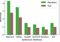
Baselines In the convex setting, we compare the performance of AdaCore with Craig (Mirzasoleiman et al., 2020) that extracts subsets that approximate the full gradient, as well as Random subsets. For non-convex experiments, we additionally compare AdaCore with GradMatch and Glister (Killamsetty et al., 2021, 2020). For AdaCore and Craig, we use the gradient w.r.t the input to the last layer, and for Glister and GradMatch we use the gradient w.r.t the penultimate layer, as specified by the methods. In all cases, we select subsets separately from each class proportional to the class sizes, and train on the union of the subsets. We report average test accuracy across 3 trials in all experiments.
5.1 Convex Experiments
In our convex experiments, we apply AdaCore to select a coreset to classify the Ijcnn1 dataset using L2-regularized logistic regression: . Ijcnn1 includes 49,990 training and 91,701 test data points of 22 dimensions, from 2 classes with 9-to-1 class imbalance ratio. In the convex setting, we only need to calculate the curvature once to find one AdaCore subset for the entire training. Hence, we utilize the complete Hessian information, computed analytically, as discussed in Appendix B.3. We apply an exponential decay learning schedule with learning rate parameters and . For each model and method (including the random baseline) we tuned the parameters via a search and reported the best results.
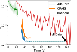
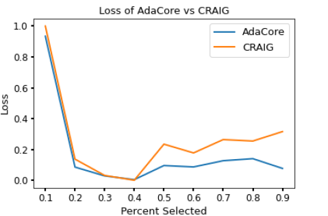
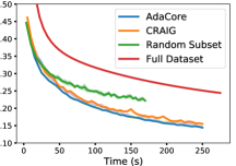
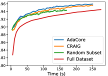
AdaCore achieves smaller loss residual with a speedup Figure 1 compares the loss residual for SGD and Newton’s method applied to coresets of size 10% extracted by AdaCore (blue), Craig (orange), and random (green) with that of full dataset (red). We see that AdaCore effectively minimizes the training loss, achieving a better loss residual than Craig and random sampling. In particular, AdaCore matches the loss achieved on the full dataset with more than a 2.5x speedup for SGD and Newton’s methods. We note that training on random 10% subsets of the data cannot effectively minimize the training loss. We show the superior performance of training with SGD on subsets of size 10% to 90% found with AdaCore vs Craig in Appendix Fig. 6.
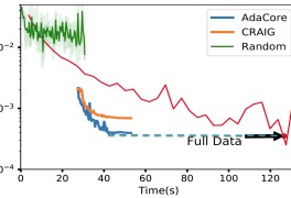
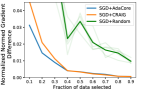
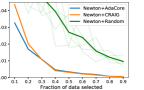
AdaCore better estimates the full gradient Fig. 2 shows the normalized gradient difference between gradient of the full data vs. weighted gradient of subsets of different sizes obtained by AdaCore vs Craig and Random, at the end of training by each method. We see that by considering curvature information, AdaCore obtains a better gradient estimate than Craig and Random subsets.
| AdaHessian | SGD+Momentum | |
| Random | ||
| Craig | ||
| GradMatch | ||
| Glister | ||
| AdaCore (no avg) | ||
| AdaCore (avg g) | ||
| AdaCore (avg H) | ||
| AdaCore | ||
| AdaCore |
5.2 Non-Convex Experiments
Datasets We use CIFAR10 (60k points from 10 classes) , class imbalanced version of CIFAR10 (32.5k points from 10 classes) and CIFAR100 (32.5k points from 100 classes) (Krizhevsky et al., 2009), BDD100k (100k points from 7 classes) (Yu et al., 2020). The results on MNIST (70k points from 10 classes) (Deng, 2012) can be found in Appendix C.6. Images are normalized to [0,1] by division with 255.
Models and Optimizers We train ResNet-20 and ResNet-18 (He et al., 2016), with convolution, average pooling and dense layers with softmax outputs and weight decay of . We use a batch size of 256 in all experiments (except Table 3, Fig. 4a), and train using SGD with momentum of 0.9 (default), or AdaHessian. For training, we use standard learning rate scheduler for ResNet starting with 0.1 and exponentially decaying by factor 0.1 at epochs 100 and 150. We used linear learning rate warm-up for the first 20 epochs to prevent weights from diverging when training with subsets. All experiments were ran on a 2.4GHz CPU and RTX 2080 Ti GPU.
Calculating the Curvature To calculate the Hessian diagonal using Eq. (8), we use a batch size of to calculate the expected Hessian diagonal over the training data. We observed that a smaller batch size provides a higher quality Hessian compared to larger batch sizes, as shown in Table 1.
Baseline Comparison and Ablation Study Table 1 shows the accuracy of training ResNet-20, using SGD with momentum of 0.9 and AdaHessian, for 200 epochs on =1% subsets of CIFAR-10 chosen every =1 epoch by different methods. For SGD+momentum, AdaCore outperforms Craig by 12%, Random by 10%, GradMatch by 6%, and Glister by 16.8%. Note that in total, AdaCore selects 74% of the dataset during the entire training process, whereas Random visits 87%. Thus, AdaCore effectively selects subsets contributing the most to generalization. We see that the accuracy gap between the baselines and AdaCore shrinks when applying more powerful optimizers such as AdaHessian. Table 1 also shows the effect of exponential averaging of gradients and Hessian diagonal, and larger batch sizes for calculating the Hessian diagonal . We see that exponential averaging help AdaCore achieving better performance, and smaller provides better results.
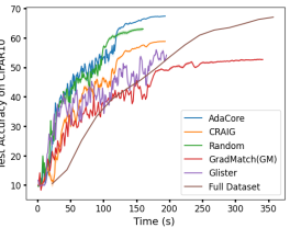
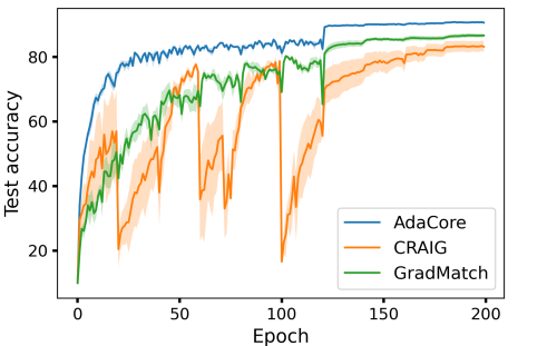
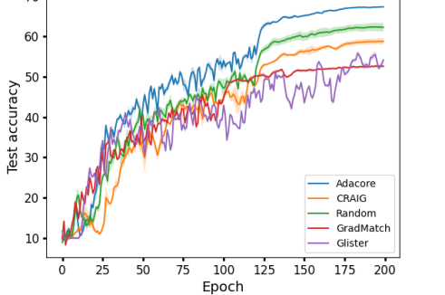
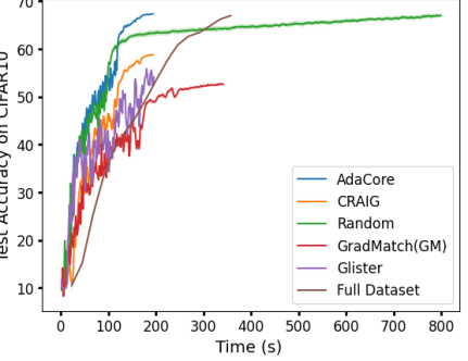
Fig. 3a compares the performance of ResNet-18 on 1% subsets selected from CIFAR-10 with different methods. We compare the performance of training on AdaCore, Craig, GradMatch, Glister, and Random subsets for 200 epochs, with training on full data for 15 epochs. This is the number of iterations required for training on the full data to achieve a comparable performance to that of AdaCore subsets. We see that training on AdaCore coresets achieves a better accuracy 2.5x faster than training on the full dataset, and more than 4.5x faster than the next best subset selection algorithm for this setting (c.f. Fig. 8b in Appendix for complete results).
| =, =20 | =, =10 | =, =5 | |
|---|---|---|---|
| AdaCore | |||
| Craig | |||
| Random | |||
| GradM | |||
| Glister |
| AdaC. | Craig | Rand |
|
|
|||||
|---|---|---|---|---|---|---|---|---|---|
|
58.32% | 56.32% | 49.14% | 1.69% | 8.91% | ||||
|
68.23% | 58.3% | 60.7% | 9.93% | 8.16% | ||||
|
66.89% | 58.17% | 65.46% | 8.81% | 1.52% |
| ResNet20, CIFAR10 = , = 20 | ResNet20, CIFAR10 = , = 20 | ResNet18, CIFAR10-IMB = , = 20 | ResNet18, CIFAR10-IMB = , = 20 | |
|---|---|---|---|---|
| AdaCore | ||||
| Craig |
Frequency and size of subsets selection Table 2, 4 shows the performance of different methods for selecting subsets of size of the data every epochs, from CIFAR-10 and imbalanced CIFAR-10. Table 2 shows that selecting subsets of size 1% every epochs with AdaCore achieves a superior performance compared to the baselines. Table 4 shows that AdaCore can successfully select larger subsets of size and outperform Craig (Std is reported in Appendix, Table 5).
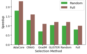
AdaCore speeds up training Fig 4 compares the speedup of various methods during training ResNet18 on 10% subsets selected every epochs from BDD 100k and CIFAR-100. All the methods are trained to achieve a test accuracy between 72% and 74% on BDD 100k, and between 57% and 50% on CIFAR-100. On BDD 100k, AdaCore achieves 74% accuracy in 100 epochs and training on full data achieves a similar performance in 45 epochs. For CIFAR-100, AdaCore achieves 59% accuracy in 200 epochs and training on full data achieves a similar performance in 40 epochs. Complete results on speedup and test accuracy of each method can be found in Appendix C.3, C.4. We see that AdaCore achieves 2.5x speedup over training on full data and 1.7x over that of training on random subsets on BDD 100k. For CIFAR-100, AdaCore achieves 4.2x speedup over training on random subsets and 2.9x over training on full data. Compared to the baselines, AdaCore can achieve achieve the desired accuracy much faster.
Effect of batch size Table 3 compares the performance of training with different batch sizes on subsets found by various methods. We see that training with larger batch size on subsets selected by AdaCore can achieve a superior accuracy. As AdaCore selects more diverse subsets with smaller weights, one can train with larger mini-batches on the subsets without increasing the gradient estimate error. In contrast, Craig subsets have elements with larger weights and hence training with fewer larger mini-batches has larger gradient error and does not improve the performance.
In summary, see that AdaCore consistently outperforms the baselines over various architectures, optimizers, subset sizes, selection frequency, and batch sizes.
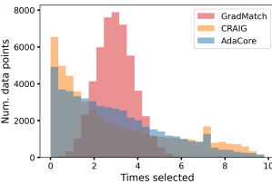
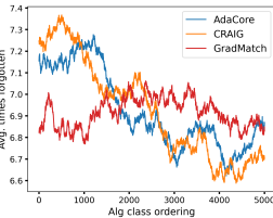
AdaCore selects more diverse subsets Fig. 3b shows the number of times different methods selected a particular elements during the entire training. We see that AdaCore successfully selects a more diverse set of examples compared to Craig. We note that GradMatch may not be able to select subsets with the desired size, and instead augments the selected subset with randomly selected examples. Hence, it has a normal-shaped distribution. Fig. 3c shows mean forgetting score for all examples within a class ranked by AdaCore at the end of training, over sliding window of size 100. We see that AdaCore prioritizes selecting less forgettable examples. This shows that indeed AdaCore is able to distinguish different groups of easier examples better, and hence can prevent catastrophic forgetting by including their representatives in the coresets.
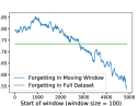
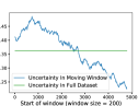


AdaCore vs Forgettability and Uncertainty Fig. 5a, 5b show mean forgettability and uncertainty in sliding windows of size 100, 200 over examples sorted by AdaCore at the end of training. We see that AdaCore heavily biases its selections towards forgettable and uncertain points, as training proceeds. Interestingly, 5a reveals that AdaCore avoids the most forgettable samples in favor of slightly more memorable ones, suggesting that AdaCore can better distinguish easier groups of examples. Figure 5b shows similar bias towards uncertain samples. Fig. 5c, 5d show the most and least selected images by AdaCore, respectively. We see the redundancies in the never selected images, whereas images frequented by AdaCore are quite diverse in color, angles, occluded subjects, and airplane models. This confirms the effectiveness of AdaCore in extracting the most crucial subsets for learning and eliminating redundancies.
6 Conclusion
We proposed AdaCore, a method that leverages the topology of the dataset to extract salient subsets of large datasets for efficient machine learning. The key idea behind AdaCore is to dynamically incorporate the curvature and gradient of the loss function via an adaptive estimate of the Hessian to select weighted subsets (coresets) which closely approximate the preconditioned gradient of the full dataset. We proved exponential convergence rate for first and second-order optimization methods applied to AdaCore coresets, under certain assumptions. Our extensive experiments, using various optimizers e.g., SGD, AdaHessian, and Newton’s method, show that AdaCore can extract higher quality coresets compared to baselines, rejecting potentially redundant data points. This speeds up the training of various machine learning models, such as logistic regression and neural networks, by over 4.5x while selecting fewer but more diverse data points for training.
Acknowledgements
This research was supported in part by UCLA-Amazon Science Hub for Humanity and Artificial Intelligence.
References
- Alain et al. (2015) Alain, G., Lamb, A., Sankar, C., Courville, A., and Bengio, Y. Variance reduction in sgd by distributed importance sampling. arXiv preprint arXiv:1511.06481, 2015.
- Allen-Zhu et al. (2016) Allen-Zhu, Z., Yuan, Y., and Sridharan, K. Exploiting the structure: Stochastic gradient methods using raw clusters. In Advances in Neural Information Processing Systems, pp. 1642–1650, 2016.
- Asi & Duchi (2019) Asi, H. and Duchi, J. C. The importance of better models in stochastic optimization. arXiv preprint arXiv:1903.08619, 2019.
- Bekas et al. (2007) Bekas, C., Kokiopoulou, E., and Saad, Y. An estimator for the diagonal of a matrix. Applied Numerical Mathematics, 57(11):1214–1229, 2007. ISSN 0168-9274. doi: https://doi.org/10.1016/j.apnum.2007.01.003. URL https://www.sciencedirect.com/science/article/pii/S0168927407000244. Numerical Algorithms, Parallelism and Applications (2).
- Bertsekas (1982) Bertsekas, D. P. Projected newton methods for optimization problems with simple constraints. SIAM Journal on control and Optimization, 20(2):221–246, 1982.
- Birodkar et al. (2019) Birodkar, V., Mobahi, H., and Bengio, S. Semantic redundancies in image-classification datasets: The you don’t need. arXiv preprint arXiv:1901.11409, 2019.
- Boyd & Vandenberghe (2004) Boyd, S. and Vandenberghe, L. Convex Optimization. Cambridge University Press, USA, 2004. ISBN 0521833787.
- Chen et al. (2001) Chen, S. S., Donoho, D. L., and Saunders, M. A. Atomic decomposition by basis pursuit. SIAM review, 43(1):129–159, 2001.
- Coleman et al. (2020) Coleman, C., Yeh, C., Mussmann, S., Mirzasoleiman, B., Bailis, P., Liang, P., Leskovec, J., and Zaharia, M. Selection via proxy: Efficient data selection for deep learning. In International Conference on Learning Representations (ICLR), 2020.
- Deng (2012) Deng, L. The mnist database of handwritten digit images for machine learning research. IEEE Signal Processing Magazine, 29(6):141–142, 2012.
- Donoho (2006) Donoho, D. L. Compressed sensing. IEEE Transactions on information theory, 52(4):1289–1306, 2006.
- Elenberg et al. (2018) Elenberg, E. R., Khanna, R., Dimakis, A. G., Negahban, S., et al. Restricted strong convexity implies weak submodularity. Annals of Statistics, 46(6B):3539–3568, 2018.
- Ghorbani & Zou (2019) Ghorbani, A. and Zou, J. Data shapley: Equitable valuation of data for machine learning. In International Conference on Machine Learning, pp. 2242–2251. PMLR, 2019.
- He et al. (2016) He, K., Zhang, X., Ren, S., and Sun, J. Deep residual learning for image recognition. In Proceedings of the IEEE conference on computer vision and pattern recognition, pp. 770–778, 2016.
- Hofmann et al. (2015) Hofmann, T., Lucchi, A., Lacoste-Julien, S., and McWilliams, B. Variance reduced stochastic gradient descent with neighbors. In Advances in Neural Information Processing Systems, pp. 2305–2313, 2015.
- Katharopoulos & Fleuret (2018) Katharopoulos, A. and Fleuret, F. Not all samples are created equal: Deep learning with importance sampling. In International conference on machine learning, pp. 2525–2534. PMLR, 2018.
- Killamsetty et al. (2020) Killamsetty, K., Sivasubramanian, D., Ramakrishnan, G., and Iyer, R. Glister: Generalization based data subset selection for efficient and robust learning. arXiv preprint arXiv:2012.10630, 2020.
- Killamsetty et al. (2021) Killamsetty, K., Sivasubramanian, D., Mirzasoleiman, B., Ramakrishnan, G., De, A., and Iyer, R. Grad-match: A gradient matching based data subset selection for efficient learning. arXiv preprint arXiv:2103.00123, 2021.
- Krizhevsky et al. (2009) Krizhevsky, A., Nair, V., and Hinton, G. Cifar-10 (canadian institute for advanced research). 2009. URL http://www.cs.toronto.edu/~kriz/cifar.html.
- Kyrillidis et al. (2013) Kyrillidis, A., Becker, S., Cevher, V., and Koch, C. Sparse projections onto the simplex. In International Conference on Machine Learning, pp. 235–243. PMLR, 2013.
- Liu et al. (2020) Liu, C., Zhu, L., and Belkin, M. Toward a theory of optimization for over-parameterized systems of non-linear equations: the lessons of deep learning. arXiv preprint arXiv:2003.00307, 2020.
- Loshchilov & Hutter (2015) Loshchilov, I. and Hutter, F. Online batch selection for faster training of neural networks. arXiv preprint arXiv:1511.06343, 2015.
- Martens & Grosse (2015) Martens, J. and Grosse, R. Optimizing neural networks with kronecker-factored approximate curvature. In International conference on machine learning, pp. 2408–2417. PMLR, 2015.
- Minoux (1978) Minoux, M. Accelerated greedy algorithms for maximizing submodular set functions. In Optimization techniques, pp. 234–243. Springer, 1978.
- Mirzasoleiman et al. (2013) Mirzasoleiman, B., Karbasi, A., Sarkar, R., and Krause, A. Distributed submodular maximization: Identifying representative elements in massive data. In Advances in Neural Information Processing Systems, pp. 2049–2057, 2013.
- Mirzasoleiman et al. (2015) Mirzasoleiman, B., Badanidiyuru, A., Karbasi, A., Vondrák, J., and Krause, A. Lazier than lazy greedy. In Twenty-Ninth AAAI Conference on Artificial Intelligence, 2015.
- Mirzasoleiman et al. (2020) Mirzasoleiman, B., Bilmes, J., and Leskovec, J. Coresets for data-efficient training of machine learning models. In International Conference on Machine Learning, pp. 6950–6960. PMLR, 2020.
- Natarajan (1995) Natarajan, B. K. Sparse approximate solutions to linear systems. SIAM journal on computing, 24(2):227–234, 1995.
- Nocedal (1980) Nocedal, J. Updating quasi-newton matrices with limited storage. Mathematics of Computation, 35(151):773–782, 1980. ISSN 00255718, 10886842. URL http://www.jstor.org/stable/2006193.
- Pilanci et al. (2012) Pilanci, M., El Ghaoui, L., and Chandrasekaran, V. Recovery of sparse probability measures via convex programming. 2012.
- Qian (1999) Qian, N. On the momentum term in gradient descent learning algorithms. Neural networks, 12(1):145–151, 1999.
- Robbins & Monro (1951) Robbins, H. and Monro, S. A stochastic approximation method. The annals of mathematical statistics, pp. 400–407, 1951.
- Schaul et al. (2013) Schaul, T., Zhang, S., and LeCun, Y. No more pesky learning rates. In International Conference on Machine Learning, pp. 343–351. PMLR, 2013.
- Schaul et al. (2015) Schaul, T., Quan, J., Antonoglou, I., and Silver, D. Prioritized experience replay. arXiv preprint arXiv:1511.05952, 2015.
- Schwartz et al. (2019) Schwartz, R., Dodge, J., Smith, N. A., and Etzioni, O. Green ai. arXiv preprint arXiv:1907.10597, 2019.
- Strubell et al. (2019) Strubell, E., Ganesh, A., and McCallum, A. Energy and policy considerations for deep learning in nlp. In Proceedings of the 57th Annual Meeting of the Association for Computational Linguistics, pp. 3645–3650, 2019.
- Tibshirani (1996) Tibshirani, R. Regression shrinkage and selection via the lasso. Journal of the Royal Statistical Society: Series B (Methodological), 58(1):267–288, 1996.
- Toneva et al. (2018) Toneva, M., Sordoni, A., des Combes, R. T., Trischler, A., Bengio, Y., and Gordon, G. J. An empirical study of example forgetting during deep neural network learning. In International Conference on Learning Representations, 2018.
- Wolsey (1982) Wolsey, L. A. An analysis of the greedy algorithm for the submodular set covering problem. Combinatorica, 2(4):385–393, 1982.
- Xu et al. (2020) Xu, P., Roosta, F., and Mahoney, M. W. Second-order optimization for non-convex machine learning: An empirical study. In Proceedings of the 2020 SIAM International Conference on Data Mining, pp. 199–207. SIAM, 2020.
- Yao et al. (2018) Yao, Z., Xu, P., Roosta-Khorasani, F., and Mahoney, M. W. Inexact non-convex newton-type methods. arXiv preprint arXiv:1802.06925, 2018.
- Yao et al. (2020) Yao, Z., Gholami, A., Shen, S., Keutzer, K., and Mahoney, M. W. Adahessian: An adaptive second order optimizer for machine learning. arXiv preprint arXiv:2006.00719, 2020.
- Yu et al. (2020) Yu, F., Chen, H., Wang, X., Xian, W., Chen, Y., Liu, F., Madhavan, V., and Darrell, T. Bdd100k: A diverse driving dataset for heterogeneous multitask learning. In IEEE/CVF Conference on Computer Vision and Pattern Recognition (CVPR), June 2020.
Appendix A Proofs of Theorems
A.1 Proof of Theorem 4.1
See 4.1
Proof.
We prove Theorem 4.1 (similarly to the proof of Newton’s method in (Boyd & Vandenberghe, 2004)) for the following general update rule for :
| (18) | |||
| (19) |
For , this corresponds to the update rule of the Newton’s method. Define . Since is -smooth, we have
| (20) | ||||
| (21) |
where in the last equality, we used
| (22) |
Therefore, using step size we have
| (23) |
Since , we have
| (24) |
and therefore decreases as follows,
| (25) |
Now for the subset, from Eq. (5) we have that . Hence, via reverse triangle inequality , and we get
| (26) |
where and are the gradient and Hessian of the subset respectively. In Eq. (26) the RHS follows from operator norms and the LHS follows from the following lower bound on the norm of the product of two matrices:
| (27) |
Hence,
| (28) |
Therefore, on the subset we have
| (29) | ||||
| (30) | ||||
| (31) |
The algorithm stops descending when . From strong convexity we know that
| (32) |
Hence, we get
| (33) |
Descent property for Equation 5 For a strongly convex function, , we have that the diagonal elements of the Hessian are positive (Yao et al., 2020). This allows the diagonal to approximate the full Hessian which has good convergence properties.
Given a function which is strongly convex and strictly smooth, we have that is upper and lower bounded by two constants and , so that , for all . For a strongly convex function the diagonal elements in diag() are all positive, and we have:
| (34) |
where represents the natural basis vectors. Therefore, the diagonal entries of are in the range . Therefore, the average of a subset of the numbers are still in the range . As such, we can prove that Eq. (10) has the same convergence rate as its full matrix counterpart, by following the same proof as Theorem 4.1.
A.2 Proof of Theorem 4.3 and 4.4
A loss function is considered -PL on a set , if the following holds:
| (35) |
where is a global minimizer. When additionally , the -PL condition is equivalent to the - condition
| (36) |
See 4.3
For Lipschitz continuous and -PL∗ condition, gradient descent on the entire dataset yields
| (37) |
and,
| (38) |
which was shown in (Liu et al., 2020).
We build upon this result to an AdaCore subset.
Proof.
For the subset we have
| (41) |
By substituting Eq. (40) we have.
| (42) | |||
| (43) | |||
| (44) | |||
| (45) |
Where we can upper bound the norm of in Eq. (43) by a constant . And Eq. (45) follows from the -PL condition from Eq. (35).
Hence,
| (46) |
Since, , for a constant learning rate we get
| (47) |
∎
See 4.4 For Lipschitz continuous and -PL∗ condition, gradient descent on the entire dataset yields
| (48) |
and,
| (49) |
which was shown in (Liu et al., 2020).
We build upon this result to an AdaCore subset.
Proof.
For the subset we have
| (52) |
Fixing and taking expectation with respect to the randomness in the choice of the batch (noting that those indices are i.i.d.), we have
| (53) | ||||
| (54) | ||||
| (55) |
We can upper bound the norm of in Eq. (45) by a constant . And Eq. (45) follows from the -PL condition from Eq. (35) and assuming .
| (56) | |||
| (57) | |||
| (58) | |||
| (59) |
By optimizing the quadratic term in the upper bound with respect to we get .
| (60) |
Hence,
| (61) |
∎
A.3 Discussion on Greedy to Extract Near-optimal Coresets
As discussed in Section 4.4, a greedy algorithm can be applied to find near-optimal coresets that estimate the general descent direction with an error of at most by solving the submodular cover problem Eq. (13). For completeness, we include the pseudocode of the greedy algorithm in Algorithm 1. The AdaCore algorithm is run per class.
Appendix B Bounding the Norm of Difference Between Preconditioned Gradients
B.1 Convex Loss Functions
We show the normed difference for ridge regression. Similar results can be deduced for other loss functions such as square loss (Allen-Zhu et al., 2016), logistic loss, smoothed hinge losses, etc.
For ridge regression , we have . Furthermore for invertable Hessian H, let and . Therefore,
| (62) |
| (63) | |||
| (64) | |||
| (65) | |||
| (66) | |||
| (67) | |||
| (68) | |||
| (69) | |||
| (70) |
In Eq. (70) we have the norm of the inverse of the Hessian matrix. Since H is invertible we have min
| (71) | |||
| (72) |
where the substitution was made, and utilized that since H is invertible. Hence,
| (73) | |||
| (74) |
For , and .
Assuming that is bounded for all , an upper bound on the euclidean distance between preconditioned gradients can be precomputed.
B.2 Neural Networks
We closely follow proofs from (Katharopoulos & Fleuret, 2018) and (Mirzasoleiman et al., 2020) to show that we can bound the difference between the Hessian inverse preconditioned gradients of an entire NN up to a constant of the difference between the Hessian inverse preconditioned gradients of the last layer of the NN, between arbitrary datapoints and .
Consider an -layer perceptron, where is the weight matrix for the layer with hidden units. Furthermore assume is a Lipschitz continuous activation function. Then we let,
| (75) | ||||
| (76) | ||||
| (77) |
With,
| (78) | ||||
| (79) |
We have,
| (80) | ||||
| (81) | ||||
| (82) | ||||
| (83) | ||||
| (84) | ||||
From (Katharopoulos & Fleuret, 2018), (Mirzasoleiman et al., 2020), we have that the variation of the gradient norm is mostly captured by the gradient of the loss function with respect to the pre-activation outputs of the last layer of our neural network. Here we have a similar result, where, the variation of the gradient preconditioned on the inverse of the Hessian norm is mostly captured by the gradient preconditioned on the inverse of the Hessian of the loss function with respect to the pre-activation outputs of the last layer of our neural network. Assuming is bounded, we get
| (85) |
where are constants. The above holds for an affine operation followed by a slope-bounded non-linearity .
B.3 Analytic Hessian for Logistic Regression
Here we provide the analytical formulation of the Hessian of the binary cross entropy loss per data point with respect to weights for Logistic Regression.
For Binary Logistic Regression we have a loss function defined as:
| (86) |
and is the sigmoid function.
We form a Hessian matrix for each data point based on loss function as follows:
This allows us to analytically form the Hessian information per point which is needed to precompute a single coreset which will be used throughout training of the convex regularized logistic regression problem.
Appendix C Further Empirical Evidence
C.1 AdaCore estimates full gradient closely, reaching smaller loss
AdaCore obtains a better estimate of the preconditioned gradient by considering curvature and gradient information compared to the state-of-the-art algorithm Craig and random subsets. This is quantified by calculating the difference between weighted gradients of coresets and the gradient of the complete dataset.
Fig 6, shows the difference in loss reached by AdaCore vs Craig over different subset sizes. This shows that corsets selected using AdaCore to classify the Ijcnn1 dataset using logistic regression can reach a lower loss over varying subset sizes than Craig.
C.2 Class imbalance CIFAR-10
To provide further empirical evidence, we include results using a class-imbalanced version of the CIFAR-10 dataset for ResNet18. We skewed the class distribution linearly, keeping of class 9, of class 8 … of class 1, and of class 0, and trained for 200 epochs. Selecting a coreset for every epoch can be computationally expensive; instead, one can compute a coreset once every epochs. Here we investigate AdaCore’s performance on various values. As Table 5 shows, AdaCore can withstand class imbalance much better than Craig and randomly selected subsets. When , AdaCore achieves final test accuracy, above Craig, above Random, 27.4% above GradMatch and 36.2% above Glister.
| Accuracy | |||
|---|---|---|---|
| AdaCore | |||
| Craig | |||
| Random | |||
| GradMatch | |||
| Glister |
Not only is AdaCore able to outperform Craig, random, GradMatch, and Glister, but it can do so while selecting a smaller fraction of the data points during training, as shown under all settings in Table 5.
C.3 Class imbalance BDD100k
Additionally, we compared AdaCore to Craig and random selection for the BDD100k dataset, which has seven inherently imbalanced classes and 100k data points. We train ResNet50 with SGD + momentum for 100 epochs choosing subset size (s = 10%) every (R = 20) epochs on the weather prediction task. We see that AdaCore can outperform Craig by 2% and random by 8.8% seen in Table 6.
| SGD + Momentum Accuracy | S = 10% R = 20 |
|---|---|
| AdaCore | 74.3% |
| Craig | 72.3% |
| Random | 65.5% |
Additionally, Table 7 shows that AdaCore outperforms baseline methods on BDD100k providing 2.3x speedup vs. training on the entire dataset and a 1.8x speedup vs. random. We see that Craig, GradMatch & Glister do not reach the accuracy of AdaCore even given more time and epochs. The epoch value is seen in parenthesis by accuracy. These experiments were run with SGD+momentum.
| BDD100k | Speedup over | |||||||||
|---|---|---|---|---|---|---|---|---|---|---|
|
|
|
Rand | Full | ||||||
| AdaCore | 7331 | 1.8 | 2.3 | |||||||
| Craig | 10996 | 1.3 | 1.6 | |||||||
| Random | 13050 | 1 | 1.2 | |||||||
| GradMatch | 14040 | .7 | 1.1 | |||||||
| Glister | 12665 | 1.03 | 1.2 | |||||||
| Full Dataset | 16093 | 0.8 | 1 | |||||||
C.4 CIFAR-100
Table 8 shows that AdaCore outperforms baseline methods on CIFAR100, providing 4x speedup vs. training on the entire dataset and a 3.8x speedup vs. Random. We see that Craig, GradMatch and Glister do not reach the accuracy of AdaCore even given more time and epochs. The epoch value is seen in parenthesis by accuracy. These experiments were run with SGD+momentum.
| CIFAR100 | Speedup over | |||||||||
|---|---|---|---|---|---|---|---|---|---|---|
|
|
|
Rand | Full | ||||||
| AdaCore | 58.8%(200) | 341 | 4.3 | 2.8 | ||||||
| Craig | 57.3%(250) | 426 | 3.5 | 2.2 | ||||||
| Random | 58.1%(864) | 1470 | 1 | 0.65 | ||||||
| GradMatch | 57%(200) | 980 | 1.5 | 0.97 | ||||||
| Glister | 56%(300) | 1110 | 1.3 | 0.86 | ||||||
| Full Dataset | 59% (40) | 960 | 1.5 | 1 | ||||||
C.5 When first order coresets fail, continued
By preconditioning with curvature information, AdaCore is able to magnify smaller gradient dimensions that would otherwise be ignored during coreset selection. Moreover, it allows AdaCore to include points with similar gradients but different curvature properties. Hence, AdaCore can select more diverse subsets compared to Craig as well as GradMatch. This allows AdaCore to outperform first order coreset methods in many regimes, such as when subset size is large (e.g. 10%) and for larger batch size (e.g. 128).
In addition to the results shown in Figure 3a, (reproduced here as Fig 8a) where , AdaCore outperforms Craig as well as GradMatch when we increase the coreset selection period . Fig 7 shows that for larger , first-order methods succumb to catastrophic forgetting each time a new subset is chosen, whereas AdaCore achieves a smooth rise in classification accuracy. This increased stability between coresets is another benefit of AdaCore’s greater selection diversity. Interestingly, AdaCore achieves higher final test accuracy while selecting a smaller fraction of data points to train on during the training than Craig. Note that since AdaCore takes curvature into account while selecting the coresets, it can successfully select data points with a similar gradient but different curvature properties and extract a more diverse set of data points than Craig. However, as the coresets found by AdaCore provide a close estimation of the full preconditioned gradients for several epochs during training, the number of distinct data points selected by AdaCore is smaller than Craig.
C.6 MNIST
For our MNIST classifier, we use a fully-connected hidden layer of 100 nodes and ten softmax output nodes; sigmoid activation and L2 regularization with and mini-batch size of 32 on the MNIST dataset of handwritten digits containing 60,000 training and 10,000 test images all normalized to [0,1] by division with 255. We apply SGD with a momentum of 0.9 to subsets of size 40% of the dataset chosen at the beginning of each epoch found by AdaCore, CRAIG, and random. Fig 9 compares the training loss and test accuracy of the network trained on coresets chosen by AdaCore, CRAIG, and random, with that of the entire dataset. We see that AdaCore can benefit from the second-order information and effectively finds subsets that achieve superior performance to that of baselines and the entire dataset. At the same time, it achieves a 2.5x speedup over training on the entire dataset.
C.7 How batch size affects coreset performance
We see in Table 9 that training with larger batch size on subsets selected by AdaCore can achieve a superior accuracy. We reproduce Table 3 here with standard deviation values.
| AdaCore | Craig | Rand |
|
|
|||||
|---|---|---|---|---|---|---|---|---|---|
|
|||||||||
|
|||||||||
|
C.8 Potential Social Impacts
Regarding social impact, our coreset method can outperform other methods in accuracy while selecting fewer data points over training and providing over 2.5x speedup. This will allow for a more efficient learning pipeline resulting in a lesser environmental impact. Our method can significantly decrease the financial and environmental costs of learning from big data. The financial costs are due to expensive computational resources, and environmental costs are due to the substantial energy consumption and the produced carbon footprint.