Adaptive Split Balancing for Optimal Random Forest
Abstract
In this paper, we propose a new random forest algorithm that constructs the trees using a novel adaptive split-balancing method. Rather than relying on the widely-used random feature selection, we propose a permutation-based balanced splitting criterion. The adaptive split balancing forest (ASBF), achieves minimax optimality under the Lipschitz class. Its localized version, which fits local regressions at the leaf level, attains the minimax rate under the broad Hölder class of problems for any and . We identify that over-reliance on auxiliary randomness in tree construction may compromise the approximation power of trees, leading to suboptimal results. Conversely, the proposed less random, permutation-based approach demonstrates optimality over a wide range of models. Although random forests are known to perform well empirically, their theoretical convergence rates are slow. Simplified versions that construct trees without data dependence offer faster rates but lack adaptability during tree growth. Our proposed method achieves optimality in simple, smooth scenarios while adaptively learning the tree structure from the data. Additionally, we establish uniform upper bounds and demonstrate that ASBF improves dimensionality dependence in average treatment effect estimation problems. Simulation studies and real-world applications demonstrate our methods’ superior performance over existing random forests.
1 Introduction
Renowned for their empirical success, random forests are the preferred method in numerous applied scientific domains. Their versatility has greatly contributed to their popularity, extending well beyond conditional mean problems to include quantile estimation [36], survival analysis [30, 29], and feature selection [24, 37, 34, 33, 4]. Despite its widespread use, the theoretical analysis remains largely incomplete, even in terms of minimax optimality.
Consider estimating the conditional mean function for any , where is the response and is the covariate vector. Let be independent and identically distributed (i.i.d.) samples, with . Let be the random forest estimate constructed from . This paper focuses on the integrated mean squared error (IMSE) , where the expectation is taken with respect to the new observation .
Breiman’s original algorithm [8] is based on Classification And Regression Trees (CART) [9]. Its essential components, introduce auxiliary randomness through bagging and the random feature selection and play a crucial role in the algorithm’s effectiveness. At each node of every tree, the algorithm optimizes Ginny index (for classification) or prediction squared error (for regression) by selecting axes-aligned splitting directions and locations from a subset of randomly chosen set of features, using a subset of samples. The overall forest is obtained by averaging over an ensemble of trees. [42] established consistency of Breiman’s original algorithm under additive models with continuous components, but did not specify a rate. Recently, [14] established the rate under a “sufficient impurity decrease” (SID) condition for high dimensional setting, and [32] extended this to cases where covariates’ dimension grows sup-exponentially with the sample size. These results suggest that Breiman’s original algorithm retains consistency with discontinuous conditional mean functions and high-dimensional covariates. However, the established consistency rates for smooth functions were observed to be slow. For instance, for simple linear functions, the rates are no faster than and , respectively; see Table 1.1. Given the theoretical complexities associated with CART-split criterion, [5]111The results presented by [5] necessitate prior knowledge of the active features, information that is typically unknown in practice. As an alternative, the author also suggested the honest technique albeit without providing any theoretical guarantees., [1], and [31] investigated a simplified version named the “centered forest,” where the splitting directions are chosen randomly, and splitting points are selected as midpoints of parent nodes. A more advanced variant, the “median forest,” [31, 17], selects sample medians as splitting points. Importantly, both centered and median forests’ consistency rates are slow, with minimax rates attained only when ; see Table 1.1 and Figure 1.
| Methods | Consistency rate | Functional class | Random Forest | Splitting criterion |
|---|---|---|---|---|
| [23] | , | Purely uniform | Data-independent | |
| [5] | -sparse | Centered | Data-independent | |
| [1] | , | Centered | Data-independent | |
| , | , | |||
| [38] | , | Mondrian | Data-independent | |
| [40] | , , | Tessellation | Data-independent | |
| [12] | , , | Debiased Mondrian | Data-independent | |
| [10] | , , | Extrapolated tree | Data-independent | |
| [31] | , | Centered | Data-independent | |
| Median | Unsupervised | |||
| [17] | Median | Unsupervised | ||
| [42] | Only | Additive model | Breiman | Supervised |
| [32] | Additive model | Breiman | Supervised | |
| [14] | , , | SID(, | Breiman | Supervised |
| [3] | , | Honest | Unsupervised if , | |
| , | supervised if | |||
| [19] | , | Local linear honest | Supervised | |
| , | ||||
| This paper | ASBF | Unsupervised if , | ||
| , , | L-ASBF | supervised if |
Centered forests and other “purely random forests” [38, 40, 6, 1, 31], grow trees independently from all the samples. Few studies among these have achieved minimax rates for smooth functions. [21] achieved near-minimax rates exclusively for Lipschitz functions by using an “early stopping” technique, though their splitting criterion remains data-independent. Mondrian forests [38] attain IMSE minimax optimal rate for the Hölder class when . [40] introduced Tessellation forests, extending minimax optimality to . [12] proposed debiased Mondrian forests, establishing minimax optimal rates any and in the point-wise mean squared error (MSE) for fixed interior points. However, this debiasing procedure only corrects for interior bias and not boundary bias, preventing it from achieving minimax optimality in terms of the IMSE. [10] allows arbitrary and established nearly optimal in-sample excess risk; however, they did not provide upper bounds for the out-of-sample IMSE. All aforementioned works use data-independent splits, restricting the use of data during tree growth. As a result, purely random forests lose the unique advantages of tree-based methods.
Recently, [3, 47, 46, 19] explored “honest forest” variant that differs from Breiman’s forest in two key aspects: (a) the splitting point ensures that child nodes contain at least fraction of parent’ samples, and (b) the forest is “honest” using two independent sub-samples per tree. One sub-sample’s outcomes and all the covariates, are used for splitting, while the other sub-sample’s outcomes are used for local averaging. Now, the splits depend on both the covariates and outcomes as long as . For , their method degenerates to the median forest. Without the -fraction constraint, splits tend to concentrate at the parent node endpoints, resulting in inaccurate local averaging; see [28, 9, 11]. However, the consistency rates for honest forests remain sub-optimal; see Table 1.1 and Figure 1.
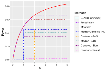
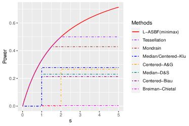
We aim to improve upon the existing methods, which either fail to achieve minimax rates or do not fully utilize the data’s information. To address these limitations, we propose a new splitting criterion that eliminates the auxiliary randomness of the random feature selection. Instead, our approach employs a permutation-based splitting criterion that balances the depth of the tree branches, resulting in minimax optimal rates in simple, smooth situations. Detailed construction is deferred to Algorithm 1. A special case of the proposed method is balanced median forest which attains the minimax optimal rate for Lipschitz continuous functions. We propose a local ASBF (L-ASBF) for the Hölder class , that performs -th order local polynomial regression within the terminal leaves for any . A specific case is the local linear approach of [19], where now the addition of balanced splitting ensures a faster convergence rate; see Table 1.1. We show that the L-ASBF reaches minimax optimality over the broad Hölder class for any and . To the best of our knowledge, this marks the first random forest that attains minimax optimal rates in terms of the IMSE for the Hölder smoothness class with any and , as seen in Figure 1. We also derive uniform rates and demonstrate minimax optimality for any ; see in Section 3.3.
Random forests have been extensively applied to causal inference, with much of the literature focusing on estimating the conditional average treatment effect (CATE); see [46, 3]. Estimating the average treatment effect (ATE), however, poses unique challenges; see Remark 1. We use ASBF with augmented inverse propensity weighting (AIPW) to estimate ATE. In contrast to existing random forest methods for which ATE inferential guarantees would confine feature dimensions to one, our methods advance the field. They support multi-dimensional features, therefore significantly broadening the practical applications for forest-based ATE inference.
2 Adaptive Split Balancing Forest
The regression tree models function by recursively partitioning the feature space into non-overlapping rectangles, generally called leaves or nodes. For any given point , a regression tree estimates using the average of responses for those samples in the same leaf as : , where denotes all the auxiliary randomness in the tree-growing process and is independent of the samples, denotes the support of , is the indices of training samples used for local averaging and possibly depends on , and represents the terminal leaf containing the point .
Random forests consider ensembles of regression trees, where the forests’ predictions are the average of all the tree predictions. Let denote the collection of regression trees in a forest, where is the number of trees and are i.i.d. auxiliary variables. For any , random forests estimate the conditional mean as where for any function , denotes the empirical average over the auxiliary variables, and we omit the dependence of such an expectation on for the sake of notation simplicity. Using the introduced notations, random forests can also be represented as a weighted average of the outcomes:
| (2.1) |
To study the estimation rates of random forests, we consider the following decomposition of IMSE: where is the stochastic error originating from the random noise , and is the approximation error. Let be the minimum leaf size. Standard techniques lead to ; see (LABEL:thm:balance_eq2) of the Supplement. The control of the remaining approximation error is the key to reaching an optimal overall IMSE.
2.1 Auxiliary randomness and approximation error
We focus on the Lipschitz class here, with the Hölder class explored in Section 3. In the following, we illustrate how the auxiliary randomness introduced by the widely-used random feature selection affects the approximation error of tree models.
Assumption 1 (Lipschitz continuous).
Assume that satisfies for all with some constant .
For any leaf , let be its diameter. Under the Lipschitz condition, the approximation error can be controlled by the leaves’ diameters: Therefore, it suffices to obtain an upper bound for the diameters. Although the Breiman’s algorithm selects up to features at random, we find it worthwhile to study the special case with , as seen in centered and median forests. Recall that in the centered forest, a splitting direction is randomly selected (with probability ) for each split, and the splitting location is chosen as the center point of the parent node. For the moment, let , meaning the forest is the ensemble of infinitely many trees. Suppose that each terminal leaf has been split for times, and consider a sequence of consecutive leaves containing , with the smallest (terminal) leaf denoted as .
For each and , let if the -th split is performed along the -th coordinate, and otherwise. Here, and represent the corresponding probability measure and the expectation taken with respect to , respectively. For any given , the sequence is i.i.d., with for centered forest. Let be the length of the longest segment parallel to the -th axis that is a subset of . Then,
| (2.2) |
The discrepancy introduced by the strict inequality (i),“Jensen gap”, stems from the variation in the quantity , representing the count of splits along the -th direction induced by the auxiliary randomness . This discrepancy results in a relatively large approximation error (up to logarithmic terms). By selecting an optimal (or ) that strikes a balance between stochastic and approximation errors, the centered forest yields an overall IMSE of the size – which is not minimax optimal for Lipschitz functions as long as , as depicted in Figure 1.
The sub-optimality stems from the forests’ excessive reliance on auxiliary randomness, leading to a significant number of redundant and inefficient splits. When splitting directions are chosen randomly, there is a non-negligible probability that some directions are overly selected while others are scarcely chosen. Consequently, terminal leaves tend to be excessively wide in some directions and overly narrow in others. For centered and median forests, this long and narrow leaf structure is solely due to auxiliary randomness and is unrelated to the data. This prevalence of long and narrow leaves increases the expected leaf diameter, resulting in a significant approximation error that deviates from the optimal one. Averaging across the trees stabilizes the forest, but to attain minimax optimal rates, controlling the number of splits at the tree level is essential to mitigate the Jensen gap, as shown in (2.2).
Instead of selecting splitting directions randomly, we adopt a permutation-based and more balanced approach. By ensuring a sufficiently large for each and reducing dependence on auxiliary randomness , we achieve an approximation error of , as shown in Lemma 2.1. This upper bound mirrors the right-hand side of (2.2) (whereas centered or median forests cannot improve the left-hand side) when , resulting in a minimax optimal rate for the overall IMSE when (or ) is chosen to balance the approximation and the stochastic error.
2.2 Adaptive Split Balancing
In order to reduce the large approximation error caused by auxiliary randomness, we propose a permutation-based splitting method. Each time a leaf is split, we randomly select a direction from one of the sides that has been split the least number of times. Moreover, the splitting directions are chosen in a balanced fashion – we have to split once in each direction on any given tree path before proceeding to the next round.
| (2.3) | |||
| (2.4) |
| (2.5) |
To further enhance the practical performance, we employ data-dependent splitting rules of the “honest forests” approach that are dependent on both and . This flexibility is particularly valuable when the local smoothness level varies in different directions and locations. For each tree, we partition the samples into two sets, denoted by and . Additionally, we impose constraints on the child node -fraction and terminal leaf size . With and , we require the following conditions to hold: (a) each child node contains at least an -fraction of observations within the parent node, and (b) the number of observations within terminal leaves is between and . The splitting locations are then determined to minimize the empirical mean squared error (or maximize the impurity gain) within each parent node, selected from the set of points satisfying the above conditions. For more details, refer to Algorithm 1 and an illustration in Figure 2.
Any controls the balance in leaf lengths, and any prevents greedy splits near the endpoints of the parent node. For any , while the terminal leaves may still vary in width, they will be more balanced than before, hence the term “adaptive split-balancing.” Unlike centered and median forests, this time, the long and narrow leaf structure depends on the data. This distinction sets it apart from methods with data-independent splitting rules (e.g., [38, 40, 21]), allowing us to improve empirical performance, particularly when covariates have distinct local effects on the outcome.
While Algorithm 1 selects splitting points data-dependently and can adaptively learn local smoothness levels for different directions, it still encounters challenges in the presence of certain sparse structures. Notably, even if some covariates are entirely independent of the outcome, Algorithm 1 may still make splits along such directions. These splits are redundant, as they do not contribute to reducing the approximation error but increase the stochastic error, due to the smaller sample sizes in the resulting child nodes.
To address sparse situations, we introduce a tuning parameter, , representing the number of candidate directions for each split. Unlike existing methods, we select candidate directions in a balanced fashion instead of randomly. In each round, we initiate a collection of index sets, each containing mtry distinct directions, ensuring each direction appears in exactly mtry sets. At each split, we randomly select one unused index set for the current round. Alternatively, we can achieve the same result by shuffling the directions before each round and setting the index sets as , , etc., in a random order; see Figure 3. The selected index set provides the candidate splitting directions for the current node. Details are provided in Algorithm 2.
When the true conditional mean function is sparse, setting a relatively large mtry avoids splits on redundant directions. Conversely, when all directions contribute similarly, a smaller mtry prevents inefficient splits due to sample randomness. However, existing methods select candidate sets randomly, causing some directions to be frequently considered as candidate directions. This randomness can reduce approximation power by neglecting important features. In contrast, our balanced approach ensures all features are equally considered for selection at the tree level, making all the trees perform similarly and leading to a smaller estimation error for the forest. Due to the Jensen gap, the error of the averaged forest mainly stems from the poorer-performing trees, as the approximation power non-linearly depends on the number of splits in important features. The tuning parameters (location) and mtry (direction) control the “greediness” of each split during the tree-growing procedure. Greedy splits, characterized by a small and a large mtry, lead to better adaptability but are sensitive to noise, making them sub-optimal under the Lipschitz or Hölder class. Conversely, non-greedy splits, which use a larger and a smaller mtry, achieve minimax optimal results under smooth functional classes but are non-adaptive to complex (e.g., sparse) scenarios.
2.3 Theoretical results
For simplicity, we consider uniformly distributed with support , as seen in [1, 23, 5, 31, 10, 17, 42, 19, 11, 36, 35, 46]. We first highlight the advantages of the balanced approach.
Lemma 2.1.
For any and , the leaves constructed by Algorithm 1 satisfy
The right most term of the above expression dominates the rest and determines the expected size of the diameter . Recall that the sample-splitting fraction remains constant and that the minimum node size, is such that . According to Lemma 2.1, the proposed forests’ approximation error is at the order of . Our balanced median forest, with yields a rate of , whereas, a standard median forest with random feature selection has a strictly larger rate of [31], whenever ; for , the rates are the same (no need to choose a splitting direction). Centered forests achieve comparable upper bounds, which suggests the sub-optimality of auxiliary randomness.
We further assume the following standard condition for the noise variable.
Assumption 2.
Assume that almost surely with some constant .
The following theorem characterizes the IMSE of the proposed forest in Algorithm 1.
Theorem 2.2.
The issue of excess auxiliary randomness is inherent at the tree level, meaning that merely collecting more samples or further averaging does not address the optimality of the approximation error. Our approach to resolving this involves a new splitting criterion that has yielded minimax optimal rates.
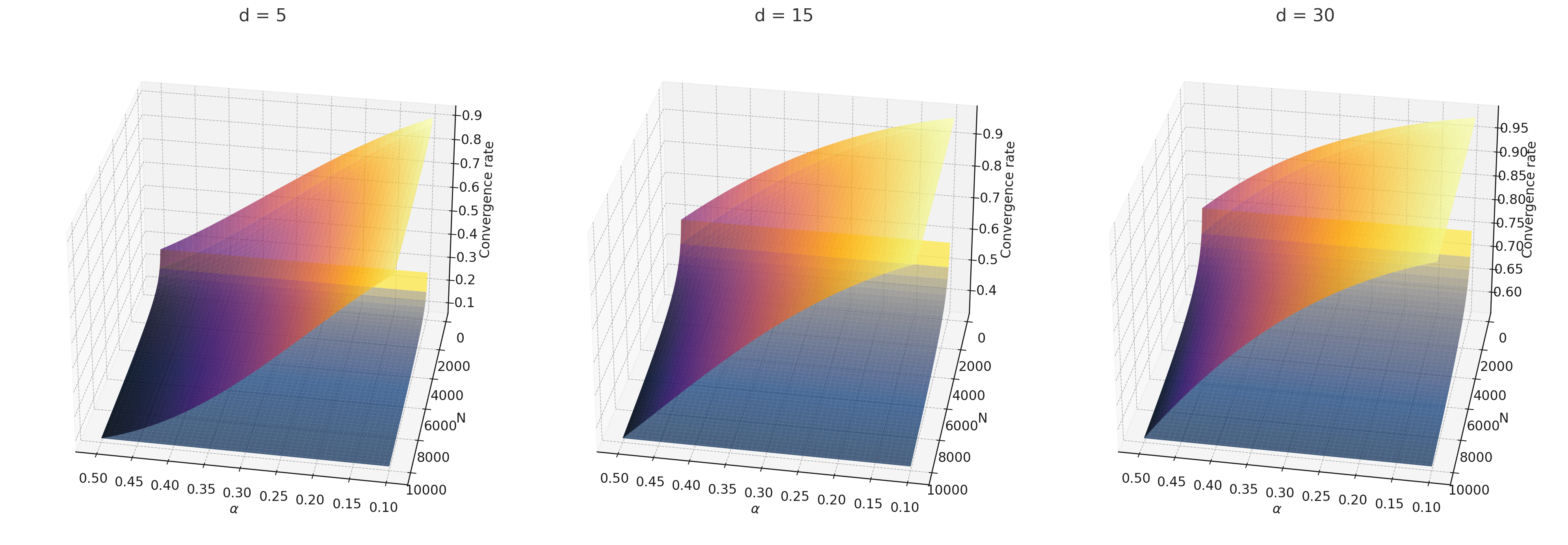
For instance, split-balancing median forest is the first minimax optimal median forest. When setting , split-balancing random forest becomes new, balanced median forest, with the optimal minimax rate of . In contrast, existing median and center forests [31, 17, 5, 1] do not achieve the minimax optimal rate; see Table 1.1 and Figure 1. The conclusions of Theorem 2.2 remain valid for any constant in the range . Greedy splits (small ) enhance adaptability by leveraging information from both and , whereas non-greedy splits attain minimax optimality, necessitating a balance in practice. The rates are represented in Figure 4.
3 Local Adaptive Split Balancing Forest
In this section, we extend our focus to more general Hölder smooth functions and introduce local adaptive split-balancing forests capable of exploiting higher-order smoothness levels.
3.1 Local polynomial forests
To capture the higher-order smoothness of the conditional mean function , we propose to fit a -th local polynomial regression within the leaves of the split-adaptive balanced forest of Section 2.2. We first introduce the polynomial basis of order . For any and , let , where . For instance, , , and . Denote as the -th order polynomial basis, where . For any , define the weights as in (2.1). Using the training samples indexed by , we consider the weighted polynomial regression:
| (3.1) |
The -th order local adaptive split balancing forest is proposed as
Unlike Algorithm 1, where local averages are used as tree predictions, our approach here involves conducting polynomial regressions within the terminal leaves. To optimize the behavior of the final polynomial regressions, we minimize the following during the leaf construction:
| (3.2) |
where with denoting the least squares estimate within the parent node , and is the average of within the child node for each . As in Section 2.2, we also require that both child nodes contain at least an -fraction of samples from the parent node. Additional specifics are outlined in Algorithm 3. Note that Algorithm 1 is a special case of Algorithm 3 with . To further improve the forests’ empirical behavior in the presence of certain sparse structures, we also introduce a generalized sparse version of the local adaptive split balancing forest following; see Algorithm 4 in the Supplement for more details.
3.2 Theoretical results with higher-order smoothness levels
Assumption 3 (Hölder smooth).
Assume that with and . The Hölder class contains all functions that are times continuously differentiable, with (a) for all and multi-index satisfying , and (b) for all and satisfying , where is a constant.
The following theorem characterizes the convergence rate of the local adaptive split balancing forest proposed in Algorithm 3.
Theorem 3.1.
When , the rate given by (3.3) is , which is minimax optimal for the Hölder class ; see, e.g., [44]. This accomplishment represents the first random forest with IMSE reaching minimax optimality when ; refer to Table 1.1 and Figure 1.
Theorem 3.1 is built upon several key technical components. To mitigate the issue of multicollinearity during local polynomial regression within terminal leaves, we first demonstrate that , where assesses the degree of multicollinearity. Here, , , and . Unlike [19], which imposes an upper bound on the random quantity by assumption, we rigorously prove that this quantity is uniformly bounded above with high probability; see the equivalent form in Lemma S.4. Additionally, by employing localized polynomial regression, we reduce the approximation error to under the Hölder class , as detailed in (LABEL:consistency:R1) of the Supplement. Together with our proposed permutation-based splitting rule, previous results on leaf diameter (Lemma 2.1) ensure a sufficiently small rate.
[38] achieved minimax optimal IMSE for and by leveraging forest structure and concentration across trees. However, for , their optimality is limited to interior points where . Our approach broadens the range of Hölder smooth functions addressed, using polynomial approximation and split-balancing to eliminate the approximation error at the tree level.
Tessellation forest of [40] addressed this boundary issue, achieving minimax optimal IMSE for and any . Theorem 3.1 further highlights that the local split-balancing median forest (with ) is minimax optimal not only for but also for any arbitrary . This signifies a major breakthrough in attaining minimax optimality for higher-order smoothness levels.
Debiased Mondrian forests by [12] achieve minimax optimality for any and , in terms of point-wise MSE at interior points. However, their results do not yield an optimal rate for the IMSE, as their debiasing technique does not extend for boundary points. Additionally, [10] achieved a nearly optimal rates for any and but their findings are limited to in-sample excess risk.
It’s important to note that while all previous works grow trees completely independently of the samples, our approach employs supervised splitting rules with after tuning, significantly enhancing forest performance. Only [7, 19] considered data-dependent splitting rules and studied local linear forests under the special case . However, [7] only demonstrated the consistency of their method, without providing any explicit rate of convergence. [19] provided asymptotic normal results at a given . However, their established upper bound for the asymptotic variance is no faster than , which is slow as the splitting directions are chosen randomly.
3.3 Uniform consistency rate
In the following, we extend our analysis to include uniform-type results for the estimation error of the forests. These are useful for our particular applications to causal inference and more broadly are of independent interest. As Algorithm 1 is a specific instance of Algorithm 3, we focus on presenting results for the latter.
To begin, we establish a uniform bound on the diameter of the leaves as follows.
Lemma 3.2.
Suppose that , , and are constants. Choose any satisfying . Then,
with probability at least and some constant .
The result in Lemma 3.2 holds for a single tree and also for an ensemble forest. In fact, obtaining uniform results for a single tree is relatively simple – it suffices to control the diameter of each terminal leaf with high probability and take the uniform bound over all the leaves, as the number of terminal leaves is at most . However, such an approach is invalid for forests – the number of all terminal leaves in a forest grows with the number of trees . Hence, such a method can be used only when is relatively small; however, in practice, we would like to set as large as possible unless constrained by computational limits. To obtain a uniform result for forests, we approximate all the possible leaves through a collection of rectangles.
Subsequently, we present a uniform upper bound for the estimation error of the forests.
Theorem 3.3.
Let Assumption 3 hold. Suppose that . Let , , and be constants. Choose any and satisfying . Then, as ,
Moreover, let , we have
Comparing with the results in Theorem 3.1, the rates above consist of additional logarithm terms. This is due to the cost of seeking uniform bounds. When , an optimally tuned leads to the rate , which is minimax optimal for sup-norms; see, e.g., [44]. To the best of our knowledge, we are the first to establish minimax optimal uniform bounds for forests over the Hölder class for any .
3.4 Application: causal inference for ATE
In this section, we apply the proposed forests to estimate the average treatment effect (ATE) in the context of causal inference. We consider i.i.d. samples , and denote as its independent copy. Here, denotes the outcome of interest, is a binary treatment variable, and represents a vector of covariates uniformly distributed in . We operate within the potential outcome framework, assuming the existence of potential outcomes and , where represents the outcome that would be observed if an individual receives treatment . The ATE is defined as , representing the average effect of the treatment on the outcome . To identify causal effects, we make the standard assumptions seen in [41, 16, 27].
Assumption 4.
(a) Unconfoundedness: . (b) Consistency: . (c) Overlap: , where is a constant and the propensity score (PS) function is defined as for any .
Define the true outcome regression function for and consider the doubly robust score function: for any ,
As the ATE parameter can be represented as , it can be estimated as the empirical average of the score functions as long as we plug in appropriate estimates of the nuisance functions . In the following, we introduce the forests-based ATE estimator using the double machine-learning framework of [13].
For any fixed integer , split the samples into equal-sized parts, indexed by . For the sake of simplicity, we assume . For each , denote . Under Assumption 4, we can identify the outcome regression function as for each . Hence, we construct using Algorithm 3, based on samples . Additionally, we also construct using Algorithm 3, based on samples . For the sake of simplicity, we denote . The number of trees and the orders of polynomial forests are chosen in advance, where we use to denote the polynomial orders considered in the estimation of for each . Further denote as the hyperparameters for estimating . To appropriately select , we further split the samples indexed by into training and validation sets. After obtaining the nuisance estimates for each , we define the ATE estimator as
While the double machine-learning framework offers a flexible and robust approach for estimating causal parameters like the ATE, the validity of statistical inference based on these methods requires careful consideration, as asymptotic normality depends on sufficiently fast convergence rates in nuisance estimation. For instance, even when minimax optimal nuisance estimation is achieved within the Lipschitz class, inference can still be inaccurate under worst-case scenarios when . To address this, we focus on the widely used random forest method and develop techniques that enhance convergence rates. By integrating the split-balancing technique with local polynomial regression, we enhance the method’s convergence rate, thereby providing solid theoretical guarantees for forest-based ATE estimation and delivering more reliable inference in practice. Additional discussion on the technical challenges can be found in Remark 1.
Now, we introduce theoretical properties of the ATE estimator.
Theorem 3.4.
Let Assumption 4 hold, , and for each , with some positive constants and . Suppose that , , and , where and for each . Let and be constants. Choose any and Moreover, let
for each . Then, as ,
and , where .
Remark 1 (Technical challenges of forest-based ATE estimation).
It is worth emphasizing that the following aspects are the main challenges in our analysis:
(a) Establish convergence rates for the integrated mean squared error (IMSE) of the nuisance estimates. As the ATE is a parameter defined through integration over the entire population, we require nuisance convergence results in the sense of IMSE; point-wise mean squared error results are insufficient. This distinguishes our work from [46, 3], which focused on the estimation and inference for the conditional average treatment effect (CATE).
(b) Develop sufficiently fast convergence rates through higher-order smoothness. The asymptotic normality of the double machine-learning method [13] requires a product-rate condition for the nuisance estimation errors. If we only utilize the Lipschitz continuity of the nuisance functions, root- inference is ensured only when . In other words, we need to establish methods that can exploit the higher-order smoothness of nuisance functions as long as . As shown in Theorem 3.4, the higher the smoothness levels are, the larger dimension we allow for.
(c) Construct stable propensity score (PS) estimates. As demonstrated in Lemma S.6 of the Supplement, as long as we ensure a sufficiently large minimum leaf size for the forests used in PS estimation, we can guarantee that each terminal leaf contains a non-negligible fraction of samples from both treatment groups, provided the overlap condition holds for the true PS function as in Assumption 4. Consequently, we can stabilize the PS estimates, avoiding values close to zero.
4 Numerical Experiments
In this section, we assess the numerical performance of the proposed methods in non-parametric regression through both simulation studies and real-data analysis. Additional results for the ATE estimation problem are provided in Section B of the Supplement.
4.1 Simulations for the conditional mean estimation
We first focus on the estimation of conditional mean function . Generate i.i.d. covariates and noise for each .
Consider the following models: (a) , (b) . In Setting (a), we utilize the well-known Friedman function proposed by [20], which serves as a commonly used benchmark for assessing non-parametric regression methods [50, 26, 35]. We set the covariates’ dimension to and consider sample sizes . In Setting (b), we investigate the performance of the forests under various sparsity levels, keeping , , and choosing .
We implement the proposed adaptive split balancing forest (ASBF, Algorithm 1), local linear adaptive split balancing forest (LL-ASBF, Algorithm 3 with ), and local quadratic adaptive split balancing forest (LQ-ASBF, Algorithm 3 with ). In Setting (b) where various sparsity levels are considered, we further evaluate the numerical performance of the sparse adaptive split balancing forest (S-ASBF, Algorithm 2), which is more suitable for scenarios with sparse structures. We choose and utilize of samples for training purposes, reserving the remaining for validation to determine the optimal tuning parameters , as well as mtry for the sparse versions. For the sake of simplicity, we fix the honest fraction and do not perform additional subsampling.
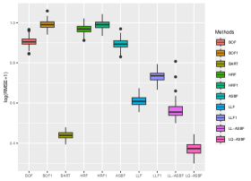
We also consider Breiman’s original forest (BOF), honest random forest (HRF), local linear forest (LLF), and Bayesian additive regression trees (BART). BOF is implemented using the R package ranger [49], HRF and LLF are implemented using the R package grf [45], and BART is implemented by the BART package [43]. HRF and LLF methods involve the tuning parameter , denoting the number of directions tried for each split. For comparison purposes, we also consider modified versions with fixed . This corresponds to the case where splitting directions are randomly chosen and is the only case that has been thoroughly studied theoretically [46, 19]. We denote the modified versions of HRF and LLF as HRF1 and LLF1, respectively. The only difference between HRF1 and the proposed ASBF is that ASBF considers a balanced splitting approach for the selection of splitting directions, instead of a fully random way; a parallel difference exists between LLF1 and LL-ASBF. Additionally, we also introduce a modified version of BOF with the splitting direction decided through random selection, denoted as BOF1.
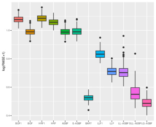
We evaluate the root mean square error (RMSE) within 1000 test points and repeat the procedure 200 times. Figures 5 and 6 depict boxplots comparing the log-transformed RMSE of all the considered methods across various settings introduced above.
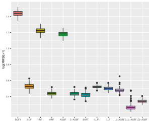
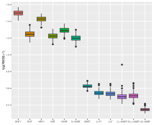
As shown in Figures 5 and 6, LQ-ASBF consistently exhibits the best performance across all the considered settings. When we focus on the choice of , the proposed ASBF method consistently outperforms the other local averaging methods BOF1 and HRF1, highlighting the distinct advantages offered by our balanced method in contrast to random feature selection. In addition, when the true model is dense, as shown in Figures 5 and 6(c), the ASBF method (with a fixed ) outperforms the general BOF and HRF methods, even when their mtry parameters are appropriately tuned. The only exception is when under Setting (a), where ASBF and BOF show similar performance. In sparse scenarios, as demonstrated in Figures 6(a)-(b), the proposed generalized sparse version S-ASBF, with an appropriately tuned mtry, clearly outperforms ASBF, especially when the sparsity level is small. Overall, the S-ASBF method consistently leads to a smaller RMSE than BOF and HRF methods in Figure 6 for all considered sparsity levels. The only exception occurs when , where S-ASBF and HRF exhibit similar behaviors. This similarity arises because, in scenarios with a small true sparsity level, the optimal mtry parameter is close to the dimension ; otherwise, it is likely that all candidate directions are redundant for certain splits. Meanwhile, when , there is no difference between the balanced and random approaches, as we always need to consider all directions as candidate directions for each split. Lastly, for forest-based local linear methods, we observe that the proposed balanced method LL-ASBF consistently outperforms both LLF1 and LLF under all considered scenarios.
4.2 Application to wine quality and abalone datasets
We further assess the performance of the considered methods in Section 4.1 using the wine quality and abalone datasets, both available from the UCI repository [2].
The wine quality dataset comprises red and white variants of the Portuguese “Vinho Verde” wine, with 4898 observations for white and 1599 observations for red. The quality variable serves as the response, measured on a scale from 0 (indicating the worst quality) to 10 (representing the highest quality). Additionally, the dataset includes 11 continuous features. For detailed information about the data, refer to [15].
The abalone dataset consists of 1 categorical feature and 7 continuous features, along with the age of abalones determined by cutting through the shell cone and counting the number of rings. This age is treated as the response variable. The categorical feature pertains to sex, classifying the entire dataset into three categories: male (1528 observations), female (1307 observations), and infant (1342 observations). For more details, refer to [39].
| Method | BOF1 | BOF | HRF1 | HRF | ASBF | S-ASBF | BART | LLF1 | LLF | LL-ASBF | SLL-ASBF | LQ-ASBF |
| Wine (overall) | 0.830 | 0.826 | 0.833 | 0.828 | 0.808 | 0.804 | 0.824 | 0.773 | 0.767 | 0.728 | 0.725 | 0.715 |
| \hdashlineRed wine | 0.809 | 0.796 | 0.819 | 0.809 | 0.794 | 0.791 | 0.799 | 0.733 | 0.735 | 0.729 | 0.719 | 0.719 |
| White wine | 0.837 | 0.835 | 0.837 | 0.834 | 0.812 | 0.809 | 0.832 | 0.786 | 0.778 | 0.728 | 0.727 | 0.714 |
| Abalone (overall) | 2.619 | 2.629 | 2.608 | 2.600 | 2.551 | 2.550 | 2.611 | 2.557 | 2.556 | 2.539 | 2.537 | 2.497 |
| \hdashlineMale abalone | 2.685 | 2.697 | 2.687 | 2.682 | 2.679 | 2.677 | 2.717 | 2.635 | 2.633 | 2.622 | 2.622 | 2.570 |
| Female abalone | 3.063 | 3.066 | 3.019 | 3.005 | 2.990 | 2.989 | 3.004 | 2.955 | 2.957 | 2.936 | 2.931 | 2.889 |
| Infant abalone | 2.006 | 2.025 | 2.025 | 2.018 | 1.839 | 1.838 | 2.016 | 1.993 | 1.988 | 1.962 | 1.961 | 1.944 |
Based on the categorical features, we initially divide the wine quality dataset into two groups (red and white) and the abalone dataset into three groups (male, female, and infant). Random forests are then constructed based on samples within each of the sub-groups. We standardize the continuous features using min-max scaling, ensuring that all features fall within the range . Each group of the data is randomly partitioned into three parts. With a total group size of , observations are used for training, observations for validation to determine optimal tuning parameters, and the prediction performance of the considered methods is reported based on the remaining testing observations. The tree size and subsampling ratio for honesty are chosen as and in advance.
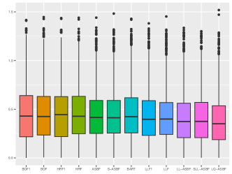
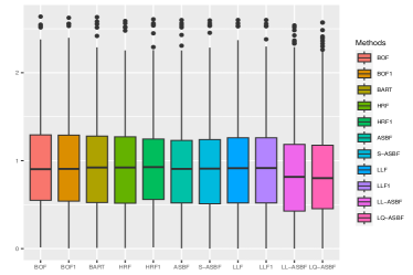
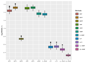
Table 4.1 reports the prediction performance of the considered random forest methods within each of the sub-groups. The proposed ASBF method and the sparse version S-ASBF outperform existing local averaging methods (including BOF, BOF1, HRF, and HRF), as well as BART, across all the sub-groups. The LL-ASBF method further outperforms existing local linear methods (LLF and LLF1), while the LQ-ASBF provides the most accurate prediction overall. Boxplots of the log-transformed absolute errors are also included in Figure 7, illustrating the overall performance for the wine quality dataset (including white and red) and the age of abalone dataset (including male, female, and infant).
5 Discussion
Since the introduction of random forest methods by [8], the infusion of randomness has played a pivotal role in mitigating overfitting and reducing the variance associated with individual greedy trees. However, this work raises pertinent concerns and queries regarding the over-reliance on such auxiliary randomness. Even for a simple median forest, opting for completely random splitting directions does not yield optimal results. Conversely, when we choose directions in a less random, or more balanced manner, we can achieve minimax results for smooth functions. Notably, as auxiliary randomness lacks information about the conditional distribution of interest, overemphasizing its role in constructing regression methods does not necessarily improve results; rather, it can compromise the approximation power of tree models. Our theoretical and numerical findings suggest that, especially for low-dimensional problems, adopting a more balanced approach in constructing trees and forests leads to more efficient outcomes. While our numerical results also indicate the efficacy of the proposed balanced method in complex scenarios, such as those involving sparse structures, further in-depth investigation is needed to understand its performance comprehensively in intricate situations.
References
- [1] S. Arlot and R. Genuer. Analysis of purely random forests bias. arXiv preprint arXiv:1407.3939, 2014.
- [2] A. Asuncion and D. Newman. UCI machine learning repository, 2007.
- [3] S. Athey, J. Tibshirani, and S. Wager. Generalized random forests. The Annals of Statistics, 47(2):1148–1178, 2019.
- [4] M. Behr, Y. Wang, X. Li, and B. Yu. Provable boolean interaction recovery from tree ensemble obtained via random forests. Proceedings of the National Academy of Sciences, 119(22):e2118636119, 2022.
- [5] G. Biau. Analysis of a random forests model. The Journal of Machine Learning Research, 13(1):1063–1095, 2012.
- [6] G. Biau, L. Devroye, and G. Lugosi. Consistency of random forests and other averaging classifiers. Journal of Machine Learning Research, 9(9), 2008.
- [7] A. Bloniarz, A. Talwalkar, B. Yu, and C. Wu. Supervised neighborhoods for distributed nonparametric regression. In Artificial Intelligence and Statistics, pages 1450–1459. PMLR, 2016.
- [8] L. Breiman. Random forests. Machine Learning, 45:5–32, 2001.
- [9] L. Breiman, J. Friedman, C. J. Stone, and R. Olshen. Classification and Regression Trees. CRC Press, 1984.
- [10] Y. Cai, Y. Ma, Y. Dong, and H. Yang. Extrapolated random tree for regression. In International Conference on Machine Learning, pages 3442–3468. PMLR, 2023.
- [11] M. D. Cattaneo, J. M. Klusowski, and P. M. Tian. On the pointwise behavior of recursive partitioning and its implications for heterogeneous causal effect estimation. arXiv preprint arXiv:2211.10805, 2022.
- [12] M. D. Cattaneo, J. M. Klusowski, and W. G. Underwood. Inference with mondrian random forests. arXiv preprint arXiv:2310.09702, 2023.
- [13] V. Chernozhukov, D. Chetverikov, M. Demirer, E. Duflo, C. Hansen, and W. Newey. Double/debiased/neyman machine learning of treatment effects. American Economic Review, 107(5):261–65, 2017.
- [14] C.-M. Chi, P. Vossler, Y. Fan, and J. Lv. Asymptotic properties of high-dimensional random forests. The Annals of Statistics, 50(6):3415–3438, 2022.
- [15] P. Cortez, A. Cerdeira, F. Almeida, T. Matos, and J. Reis. Modeling wine preferences by data mining from physicochemical properties. Decision Support Systems, 47(4):547–553, 2009.
- [16] R. K. Crump, V. J. Hotz, G. W. Imbens, and O. A. Mitnik. Dealing with limited overlap in estimation of average treatment effects. Biometrika, 96(1):187–199, 2009.
- [17] R. Duroux and E. Scornet. Impact of subsampling and tree depth on random forests. ESAIM: Probability and Statistics, 22:96–128, 2018.
- [18] H. Federer. Geometric measure theory. Springer, 2014.
- [19] R. Friedberg, J. Tibshirani, S. Athey, and S. Wager. Local linear forests. Journal of Computational and Graphical Statistics, 30(2):503–517, 2020.
- [20] J. H. Friedman. Multivariate adaptive regression splines. The Annals of Statistics, 19(1):1–67, 1991.
- [21] W. Gao, F. Xu, and Z.-H. Zhou. Towards convergence rate analysis of random forests for classification. Artificial Intelligence, 313:103788, 2022.
- [22] W. Gautschi. Some elementary inequalities relating to the gamma and incomplete gamma function. J. Math. Phys, 38(1):77–81, 1959.
- [23] R. Genuer. Variance reduction in purely random forests. Journal of Nonparametric Statistics, 24(3):543–562, 2012.
- [24] B. A. Goldstein, E. C. Polley, and F. B. Briggs. Random forests for genetic association studies. Statistical Applications in Genetics and Molecular Biology, 10(1), 2011.
- [25] W. Hoeffding. Probability inequalities for sums of bounded random variables. Journal of the American Statistical Association, 58(301):13–30, 1963.
- [26] T. Hothorn and A. Zeileis. Predictive distribution modeling using transformation forests. Journal of Computational and Graphical Statistics, 30(4):1181–1196, 2021.
- [27] G. W. Imbens and D. B. Rubin. Causal Inference in Statistics, Social, and Biomedical Sciences. Cambridge University Press, 2015.
- [28] H. Ishwaran. The effect of splitting on random forests. Machine Learning, 99:75–118, 2015.
- [29] H. Ishwaran and U. B. Kogalur. Consistency of random survival forests. Statistics & probability letters, 80(13-14):1056–1064, 2010.
- [30] H. Ishwaran, U. B. Kogalur, E. H. Blackstone, and M. S. Lauer. Random survival forests. The Annals of Applied Statistics, pages 841–860, 2008.
- [31] J. Klusowski. Sharp analysis of a simple model for random forests. In International Conference on Artificial Intelligence and Statistics, pages 757–765. PMLR, 2021.
- [32] J. M. Klusowski and P. M. Tian. Large scale prediction with decision trees. Journal of the American Statistical Association, pages 1–27, 2023.
- [33] X. Li, Y. Wang, S. Basu, K. Kumbier, and B. Yu. A debiased mdi feature importance measure for random forests. Advances in Neural Information Processing Systems, 32, 2019.
- [34] G. Louppe, L. Wehenkel, A. Sutera, and P. Geurts. Understanding variable importances in forests of randomized trees. Advances in Neural Information Processing Systems, 26, 2013.
- [35] B. Lu and J. Hardin. A unified framework for random forest prediction error estimation. The Journal of Machine Learning Research, 22(1):386–426, 2021.
- [36] N. Meinshausen and G. Ridgeway. Quantile regression forests. Journal of Machine Learning Research, 7(6), 2006.
- [37] L. Mentch and G. Hooker. Ensemble trees and CLTs: Statistical inference for supervised learning. Stat, 1050:25, 2014.
- [38] J. Mourtada, S. Gaïffas, and E. Scornet. Minimax optimal rates for mondrian trees and forests. The Annals of Statistics, 48(4):2253–2276, 2020.
- [39] W. J. Nash, T. L. Sellers, S. R. Talbot, A. J. Cawthorn, and W. B. Ford. The population biology of abalone (haliotis species) in tasmania. i. blacklip abalone (h. rubra) from the north coast and islands of bass strait. Sea Fisheries Division, Technical Report, 48:p411, 1994.
- [40] E. O’Reilly and N. M. Tran. Minimax rates for high-dimensional random tessellation forests. Journal of Machine Learning Research, 25(89):1–32, 2024.
- [41] P. R. Rosenbaum and D. B. Rubin. The central role of the propensity score in observational studies for causal effects. Biometrika, 70(1):41–55, 1983.
- [42] E. Scornet, G. Biau, and J.-P. Vert. Consistency of random forests. The Annals of Statistics, 43(4):1716–1741, 2015.
- [43] R. Sparapani, C. Spanbauer, and R. McCulloch. Nonparametric machine learning and efficient computation with bayesian additive regression trees: the bart r package. Journal of Statistical Software, 97:1–66, 2021.
- [44] C. J. Stone. Optimal global rates of convergence for nonparametric regression. The Annals of Statistics, pages 1040–1053, 1982.
- [45] J. Tibshirani, S. Athey, R. Friedberg, V. Hadad, D. Hirshberg, L. Miner, E. Sverdrup, S. Wager, M. Wright, and M. J. Tibshirani. Package ‘grf’, 2023.
- [46] S. Wager and S. Athey. Estimation and inference of heterogeneous treatment effects using random forests. Journal of the American Statistical Association, 113(523):1228–1242, 2018.
- [47] S. Wager and G. Walther. Adaptive concentration of regression trees, with application to random forests. arXiv preprint arXiv:1503.06388, 2015.
- [48] M. J. Wainwright. High-dimensional statistics: A non-asymptotic viewpoint, volume 48. Cambridge University Press, 2019.
- [49] M. N. Wright and A. Ziegler. ranger: A fast implementation of random forests for high dimensional data in C++ and R. arXiv preprint arXiv:1508.04409, 2015.
- [50] G. Zhang and Y. Lu. Bias-corrected random forests in regression. Journal of Applied Statistics, 39(1):151–160, 2012.
SUPPLEMENTARY MATERIALS FOR “ADAPTIVE SPLIT BALANCING FOR OPTIMAL RANDOM FOREST”
Notation
We denote rectangles by , where for all , writing the Lebesgue measure of as . The indicator function of a subset of a set is a function defined as if , and if . For any rectangle , we denote as the expected fraction of training examples falling within . Denote as the number of training samples falling within . For any matrix , let and denote the smallest and largest eigenvalues of the matrix , respectively. A -dimensional vector of all ones is denoted with . A tree grown by recursive partitioning is called -regular for some and if the following conditions to hold for the sample: (a) each child node contains at least an -fraction of observations within the parent node, and (b) the number of observations within terminal leaves is between and .
Appendix A The sparse local adaptive split balancing forests
In the following, we provide a generalized sparse version of the local adaptive split balancing forests proposed in Algorithm 3.
The generalized version considers an extra tuning parameter mtry, which has been also introduced in Algorithm 2, and performs local polynomial regressions within the terminal leaves as in Algorithm 3. It is worth noting that Algorithms 1-3 are all special cases of the most general version Algorithm 4.
Appendix B Simulations for the ATE estimation
In this section, we evaluate the behavior of the forest-based ATE estimator proposed in Section 3.4 through simulation studies.
We focus on the estimation of and describe the considered data generating processes below. Generate i.i.d. covariates and and noise for each . Let for each . The outcome variables are generated as . Consider the following models for the propensity score and outcomes:
-
(a)
Consider , , and .
-
(b)
Consider , , and .
| Method | Bias | RMSE | Length | Coverage | Bias | RMSE | Length | Coverage | |
|---|---|---|---|---|---|---|---|---|---|
| Setting (a): | Setting (b): | ||||||||
| BOF1 | 0.020 | 0.060 | 0.298 | 0.950 | -0.018 | 0.108 | 0.698 | 0.955 | |
| BOF | 0.020 | 0.062 | 0.303 | 0.970 | -0.012 | 0.106 | 0.714 | 0.945 | |
| HRF1 | 0.022 | 0.052 | 0.270 | 0.960 | 0.020 | 0.100 | 0.631 | 0.955 | |
| HRF | 0.018 | 0.053 | 0.270 | 0.950 | 0.015 | 0.100 | 0.634 | 0.955 | |
| ASBF | 0.016 | 0.051 | 0.263 | 0.955 | 0.011 | 0.098 | 0.627 | 0.950 | |
| \hdashlineBART | 0.022 | 0.055 | 0.269 | 0.960 | -0.015 | 0.104 | 0.632 | 0.940 | |
| LLF1 | 0.016 | 0.052 | 0.271 | 0.960 | -0.011 | 0.099 | 0.619 | 0.935 | |
| LLF | 0.015 | 0.051 | 0.271 | 0.950 | -0.016 | 0.102 | 0.622 | 0.930 | |
| LL-ASBF | 0.013 | 0.049 | 0.267 | 0.960 | -0.010 | 0.097 | 0.616 | 0.945 | |
| LQ-ASBF | 0.009 | 0.047 | 0.261 | 0.950 | -0.005 | 0.092 | 0.613 | 0.940 | |
In settings (a) and (b), we designate sample sizes as 1000 and 500, respectively, with covariate dimensions fixed at . Each setting is replicated 200 times. The results, presented in Table B.1, show that in both settings, all considered methods exhibit coverages close to the desired . In terms of estimation, the ATE estimator based on our proposed ASBF method outperforms other local averaging methods (BOF, BOF1, HRF, HRF1), as well as BART. Across both settings, we observe smaller biases (in absolute values) and RMSEs, highlighting the superior importance of the balanced technique. Furthermore, the proposed LL-ASBF consistently outperforms existing local linear methods LLF and LLF1. Notably, LQ-ASBF exhibits the best performance among the considered settings.
Appendix C Auxiliary Lemmas
Lemma S.1 (Theorem 7 of [47]).
Let and . Then, there exists a set of rectangles such that the following properties hold. Any rectangle of volume can be well approximated by elements in from both above and below in terms of Lebesgue measure. Specifically, there exist rectangles such that
Moreover, the set has cardinality bounded by
Lemma S.2 (Theorem 10 of [47]).
Suppose that , and are constants. Choose any satisfying . Let be the collection of all possible leaves of partitions satisfying -regular. Let be as defined in Lemma S.1, with and choosing as
| (C.1) |
Then, there exists an such that, for every , the following statement holds with probability at at least : for each leaf , we can select a rectangle such that , , and
Lemma S.3 (Lemma 12 of [47]).
Fix a sequence , and define the event
for any set of rectangles and threshold , where and is the number of rectangles of the set . Then, for any sequence of problems indexed by with
| (C.2) |
there is a threshold such that, for all , we have . Note that, above, , , and are all implicitly changing with .
Lemma S.4.
Suppose that , and are constants. Choose any satisfying . Then, there exists a positive constant such that the event
| (C.3) |
satisfies , where and are defined as in (LABEL:def:d_S). In addition, on the event , the matrices and are both positive-definite, and we also have
| (C.4) |
Lemma S.5.
Let the assumptions in Lemma S.4 hold. Define the event
| (C.5) |
Then, we have . Moreover, on the event , we have , and are both positive-definite, where .
In the following, we consider the average treatment effect (ATE) estimation problem and that the proposed forests provide stable propensity score estimates that are away from zero and one with high probability.
Lemma S.6.
Lemma S.6 demonstrates the stability of the inverse PS estimates, a requirement often assumed in the context of non-parametric nuisance estimates, as discussed in [13]. The above results suggest that, under the assumption of overlap, there is typically no necessity to employ any form of trimming or truncation techniques on the estimated propensities, provided the chosen tuning parameter is not too small. In fact, the parameter can also be viewed as a truncation parameter as it avoids the occurrence of propensity score estimates close to zero or one with high probability.
Appendix D Proofs of the results for the adaptive split balancing forests
Proof of Lemma 2.1.
For any and , let be the number of splits leading to the leaf , and let be the number of such splits along the -th coordinate. Define . By the balanced splitting rule, we know that the number of splits along different coordinates differs by at most one. That is, for all . Since , can be express as , with denoting the number of splits in last round if . Let be the successive nodes leading to , where and . Let be random variables denoting the number of points in located within the the successive nodes , where . Since the tree is -regular, we know that for each , and hence the following deterministic inequalities hold:
| (D.1) | |||
| (D.2) |
It follows that . Moreover, note that . Hence, we have and , which implies that
| (D.3) |