Adaptive tuning of Hamiltonian Monte Carlo methods
Abstract
With the recently increased interest in probabilistic models, the efficiency of an underlying sampler becomes a crucial consideration. A Hamiltonian Monte Carlo (HMC) sampler is one popular option for models of this kind. Performance of HMC, however, strongly relies on a choice of parameters associated with an integration method for Hamiltonian equations, which up to date remains mainly heuristic or introduce time complexity. We propose a novel computationally inexpensive and flexible approach (we call it Adaptive Tuning or ATune) that, by analyzing the data generated during a burning stage of an HMC simulation, detects a system specific splitting integrator with a set of reliable HMC hyperparameters, including their credible randomization intervals, to be readily used in a production simulation. The method automatically eliminates those values of simulation parameters which could cause undesired extreme scenarios, such as resonance artifacts, low accuracy or poor sampling. The new approach is implemented in the in-house software package HaiCS, with no computational overheads introduced in a production simulation, and can be easily incorporated in any package for Bayesian inference with HMC. The tests on popular statistical models using original HMC and generalized Hamiltonian Monte Carlo (GHMC) reveal the superiority of adaptively tuned methods in terms of stability, performance and accuracy over conventional HMC tuned heuristically and coupled with the well-established integrators. We also claim that the generalized formulation of HMC, i.e. GHMC, is preferable for achieving high sampling performance. The efficiency of the new methodology is assessed in comparison with state-of-the-art samplers, e.g. the No-U-Turn-Sampler (NUTS), in real-world applications, such as endocrine therapy resistance in cancer, modeling of cell-cell adhesion dynamics and influenza A epidemic outbreak.
keywords:
Hamiltonian Monte Carlo, GHMC, adaptive hyperparameters tuning, adaptive multi-stage splitting integration, randomization intervals, biomedical applications1 Introduction
Hamiltonian Monte Carlo (HMC) [1] has emerged as a powerful tool for sampling from high-dimensional complex probability distributions, making it invaluable in Bayesian inference applications [2]. By leveraging the Hamiltonian equations of motion for generating Monte Carlo proposals, HMC exploits gradient information on posterior distributions to enhance the convergence of the Markov chain and enables efficient exploration of the parameter space.
The Markov kernel based on Hamiltonian dynamics induces a set of hyperparameters and tuning blocks that critically impact sampling performance and include a numerical integrator for solving Hamiltonian equations, an integration step size , a number of integrations per iteration , a mass matrix . For instance, while a smaller ensures high acceptance rates and reduces computational waste, it also shortens proposal moves, increasing correlation between samples. Conversely, a larger enables longer trajectories and more independent samples but comes at the cost of increased computational overhead due to additional gradient evaluations per iteration. Consequently, significant research efforts have been devoted to identifying optimal parameter settings for HMC to balance computational efficiency and sampling performance.
Early strategies for tuning the integration step size, , focused on targeting an optimal acceptance rate for the Metropolis test [3, 4] or employing on-the-fly adaptation using primal-dual averaging algorithms [5]. Some sophisticated integration schemes have also been proposed, replacing the standard Verlet algorithm [6, 7] with more accurate multi-stage splitting integrators to enhance sampling performance and efficiency [8, 9, 10, 11, 12, 13, 14, 15]. Comprehensive reviews on numerical integration in HMC are available in [16, 17].
Regarding the number of integration steps per iteration, , a common recommendation is randomization [18, 19], though more advanced algorithms have been proposed, such as automated trajectory length selection based on the double-backing criterion [5].
Additional contributions to HMC tuning include position-dependent mass matrix adaptation [20] and methods for determining the proper number of Monte Carlo iterations to ensure convergence [21].
More recent advancements in optimization algorithms for HMC hyperparameters address both integration step size [22, 23, 24, 15, 25, 26] and number of integration steps per iteration [27, 28, 23, 25, 26].
In this study, we propose a computationally inexpensive adaptive tuning procedure that identifies an optimal numerical integrator along with a set of HMC hyperparameters tailored to a given simulation system. We call this procedure ATune and refer to an HMC method reinforced with such tuning as Adaptively-Tuned HMC (AT-HMC).
Furthermore, we extend our focus to Generalized Hamiltonian Monte Carlo (GHMC) [29, 30], a promising but relatively unexplored variant of standard HMC.
The key distinction between HMC and GHMC lies in the update mechanism for the momenta. In HMC, momenta are completely discarded after the Metropolis test and resampled at the beginnig of each iteration from a Gaussian distribution . On the contrary, GHMC performs a partial momentum update (PMU) [29]. The PMU introduces an additional hyperparameter , which, if not carefully chosen, can degrade sampling performance. This likely explains why GHMC has been less commonly used than HMC.
However, when properly tuned, GHMC can offer significant improvements in sampling accuracy and efficiency. There are two primary reasons for that.
First, in contrast to HMC, GHMC produces irreversible chains by construction [31, 2, 32]. This usually implies a faster convergence to equilibrium and a reduction in asymptotic variance [33, 34, 35, 32, 36]. Second, the partial momentum update in GHMC with a small momentum mixing angle makes a choice of the number of steps per integration leg less critical than in the case of HMC, enabling efficient sampling with shorter Hamiltonian trajectories [37], thereby enhancing both the speed and efficiency of the sampling process.
Although theoretical studies recognize potential of GHMC, little effort has been devoted to developing effective tuning strategies. Only recently, GHMC has begun to attract growing interest within the scientific community [38, 39, 40, 41].
Building on these insights, we extend our Adaptive Tuning to GHMC to derive AT-GHMC. Apart from the previously discussed in the literature choices of HMC and GHMC simulation parameters, we add to our optimal settings list randomization intervals for simulation parameters. Indeed, randomization of simulation parameters is part of any HMC-based algorithm [2], but until now its choice remains purely heuristic.
In summary, we aim to find optimal, or close to optimal choices for:
-
1.
an integration scheme for the Hamiltonian equations of motion
-
2.
a dimensional integration step size and its randomization interval
-
3.
a number of integration steps per Monte Carlo iteration and its randomization interval
-
4.
a noise control parameter (along with the appropriate randomization interval) in the PMU.
Our approach relies on the adaptive s-AIA integration method [14], which provides useful guidance on choices of integrators and optimal step size locations. According to [14], s-AIA integrators outperform the standard Velocity Verlet and other fixed-parameter multi-stage integrators in terms of both integration accuracy and their impact on sampling efficiency of HMC, for any simulation step size within a system-specific stability interval. Additionally, a key observation in [14] is that the highest performance of HMC is achieved near the center of the stability interval, provided a stability limit is accurately estimated. This also was suggested in [10, 42]. Using these findings and the analysis underlying the s-AIA approach, we identify optimal integration schemes and step size randomization intervals for both AT-HMC and AT-GHMC as well as an optimal randomization scheme for in AT-GHMC.
Moreover, we revisit the optimization strategies previously proposed for Modified HMC in [12], and adapt them to GHMC, refining the momentum refreshment procedure to derive an optimal, system-dependent noise parameter . Using the proposed settings, GHMC achieves efficient phase-space exploration even with a small number of integration steps [37].
The new tuning methodology does not incur additional computational overhead, as the optimal values are either system-specific (and can be determined a priori) or computed during a burn-in stage. Numerical experiments on standard benchmarks confirm the positive effect of proposed optimal settings on HMC and GHMC performance.
Additionally, we assess the efficiency of AT-HMC and AT-GHMC on three real-world applications, each relying on a different probabilistic model, and compare the results with those obtained using the state-of-the-art samplers commonly employed in Bayesian inference on such models. The applications include
-
1.
Patient resistance to endocrine therapy in breast cancer – a Bayesian Logistic Regression (BLR) model
-
2.
Cell-cell adhesion dynamics – a Partial Differential Equation (PDE) model
-
3.
Influenza A (H1N1) epidemics outbreak – an Ordinary Differential Equation (ODE) model.
The paper is organized as follows. Section 2 presents the essential background, covering HMC, GHMC and the numerical integration of Hamiltonian dynamics. Section 3 revisits the numerical experiments in [14], showing that optimal performance is consistently achieved near the center of a stability interval. In Section 4, we present the refined randomization interval for the optimal simulation step size and support our choice by numerical experiments.
Sections 5 and 6 introduce the optimization procedures for the random noise parameter and the number of integration steps per iteration . The Adaptive Tuning algorithm ATune is outlined in Section 7, validated on the set of benchmarks in Section 8 and systematically tested in the three real-world application studies in Section 9. Section 10 summarizes our conclusions.
2 Hamiltonian Monte Carlo
2.1 Standard formulation
Hamiltonian Monte Carlo [1] is a Markov Chain Monte Carlo (MCMC) method for obtaining correlated samples from a target probability distribution in , being the dimension of . HMC generates a Markov chain in the joint phase space with invariant distribution
| (1) |
and recovers by marginalizing out the auxiliary momentum variable (distributed according to ).
In (1), is the Hamiltonian
| (2) |
where is the symmetric positive definite mass matrix, and is the potential energy, which contains information about the target distribution :
HMC generates new proposals by alternating momentum update steps, where is drawn from a Gaussian , with the steps that update position and momenta through the numerical integration of the Hamiltonian equations
| (3) |
performed times using an explicit symplectic and reversible integrator [43]. Thus,
| (4) |
Symplecticity and reversibility of ensure that the generated Markov chain is ergodic, thus that is an invariant measure for the generated Markov chain.
Due to numerical integration errors, the Hamiltonian energy and hence the target density (1) are not exactly preserved. To address this issue, the invariance of the target density is secured through a Metropolis test with the acceptance probability
| (5) |
where
| (6) |
is the energy error resulting from the numerical integration (4). In case of acceptance, becomes the starting point for the subsequent iteration. Conversely, if the proposal is rejected, the previous state is retained for the next iteration. Regardless of acceptance or rejection, the momentum variable is discarded, and a new momentum is drawn from .
2.2 Generalized Hamiltonian Monte Carlo
Generalized Hamiltonian Monte Carlo [30] incorporates a Partial Momentum Update (PMU) [29] in standard Monte Carlo to replace the full refreshment of auxiliary momenta. The PMU reduces random-walk behavior by partially updating the auxiliary momenta through mixing with an independent and identically distributed (i.i.d) Gaussian noise :
| (7) |
Here, is a random noise parameter which determines the extent to which the momenta are refreshed. When , the update (7) reduces to the standard HMC momentum resampling scheme.
Notice that the PMU produces configurations that preserve the joint target distribution, as the orthogonal transformation in (7) maintains the distributions of . Since the momenta are not fully discarded, GHMC performs a momentum flip after each rejected proposal. As shown by Neal [2] and formally proved by Fang et al. [37], the three core steps of GHMC (Hamiltonian dynamics combined with the Metropolis test, the PMU, and momentum flip) each individually satisfy detailed balance and maintain reversibility, while their combination does not. This means that the resulting Markov chains are not reversible. Nevertheless, Fang et al. [37] demonstrated that GHMC fulfils the weaker modified detailed balance condition, ensuring the stationarity of the generated Markov chains.
2.3 Numerical integration of Hamiltonian dynamics
The most commonly used numerical scheme for solving the Hamiltonian equations (3) is the Velocity Verlet integrator [6, 7]. This scheme is widely favored due to its simplicity, good stability, and energy conservation properties. The algorithm reads
| (8) |
Here, represents the integration step size. The updates of momenta and position in (8) are often called momentum kick and position drift, respectively.
More sophisticated integration schemes have been proposed in literature, including multi-stage palindromic splitting integrators [44, 10, 45]. These methods perform multiple splits of the separable Hamiltonian system (3), applying a sequence of kicks and drifts (8) with arbitrary chosen step sizes, in contrast to the half-kick, drift, half-kick structure of the standard Verlet method. By denoting a position drift and a momentum kick, respectively, with
| (9) |
the family of -stage splitting integrators is defined as [16]
| (10) |
if , and
| (11) |
if . The coefficients , in (10)–(11) have to satisfy the conditions , and , respectively, to ensure an integration step of length . A term stage () refers to the number of gradient evaluations per integration. It is straightforward to verify that the only 1-stage splitting integrator of the form (11) is the Velocity Verlet scheme (8), which can be expressed as
| (12) |
Various choices of integration coefficients , in (10)–(11) yield integrators that reach their pick performance at different specific values of a simulation step size . To address the step size dependency, adaptive integration approaches AIA [11] and s-AIA [14] were developed for molecular simulations and Bayesian inference applications, respectively. For a given system and simulation step size , these methods select the most suitable 2- (AIA, s-AIA2) and 3- (s-AIA3) stage splitting integrator ensuring optimal energy conservation for harmonic forces. Examples of 2- and 3-stage integrators, including those used in this study, are reviewed in [10, 45, 14].
| Integrator | N. of stages () | Feature | References |
|---|---|---|---|
| Velocity Verlet | longest stability interval | [6, 7] | |
| BCSS | 2, 3 | minimizes at | [10, 45] |
| ME | 2, 3 | minimizes truncation error for | [46, 45] |
| sAIA | 2, 3 | minimizes | [14] |
3 Tracking the location of optimal step size
At first, we aim to demonstrate that top performance of HMC is typically achieved with a step size being near the center of the longest stability interval (CoLSI) for an integrator in use, as previously suggested in [42] and lately confirmed in [10] and [14]. We will use notations and for such dimensionless and dimensional step sizes, respectively. We recall that for a -stage integrator, the length of the longest dimensionless stability interval equals 2, hence, = [10, 14].
We consider the numerical experiments presented in [14] for the three benchmarks – 1000-dimensional multivariate Gaussian model, Gaussian 1 (for simplicity, from now on we call it G1000) and two BLR models, German and Musk, performed with the numerical integrators summarized in Table 1.
For each benchmark, we identify the integrator and integration step size which lead to the lowest ratio between the number of gradient evaluations, grad (which represents the bulk of the computational cost in an HMC simulation), and the minimum effective sample size [47] across variates, minESS, computed for HMC production chains of the length of iterations. Here is the number of samples in the production chains, required for reaching convergence [48, 49, 50]. We choose minESS (calculated through the effectiveSize function of the coda package of R [51]) as the most demanding one among the metrics considered in [14].
We refer to the performance metric introduced in such a way, i.e. grad/minESS, as gESS. In Section 8, we provide a detailed discussion of this metric and explore more performance metrics for validation of the proposed methodology. We emphasize that lower values of grad and higher minESS suggest faster convergence and better sampling efficiency, respectively, meaning that lower gESS indicates the improved overall performance.
Table 2 displays the best grad/minESS performance, i.e. the lowest achieved for each benchmark with -stage integrators, , and specifies the integrators along with the corresponding step sizes (normalized to the number of stages for clarity, i.e. normalized is equal to 1 for all -stage integrators) responsible for such performance. The results are visualized in Figure 1 using non-normalized step sizes.
| Benchmark | Integrator | |||
|---|---|---|---|---|
| G1000 | 2 | 6402 | 1.0 | s-AIA2 |
| 3 | 5177 | 1.1 | BCSS3 | |
| German | 2 | 28.83 | 0.9 | AIA2 |
| 3 | 26.43 | 0.8 | ME3 | |
| Musk | 2 | 249.3 | 0.8 | BCSS2 |
| 3 | 252.8 | 0.9 | s-AIA3 |
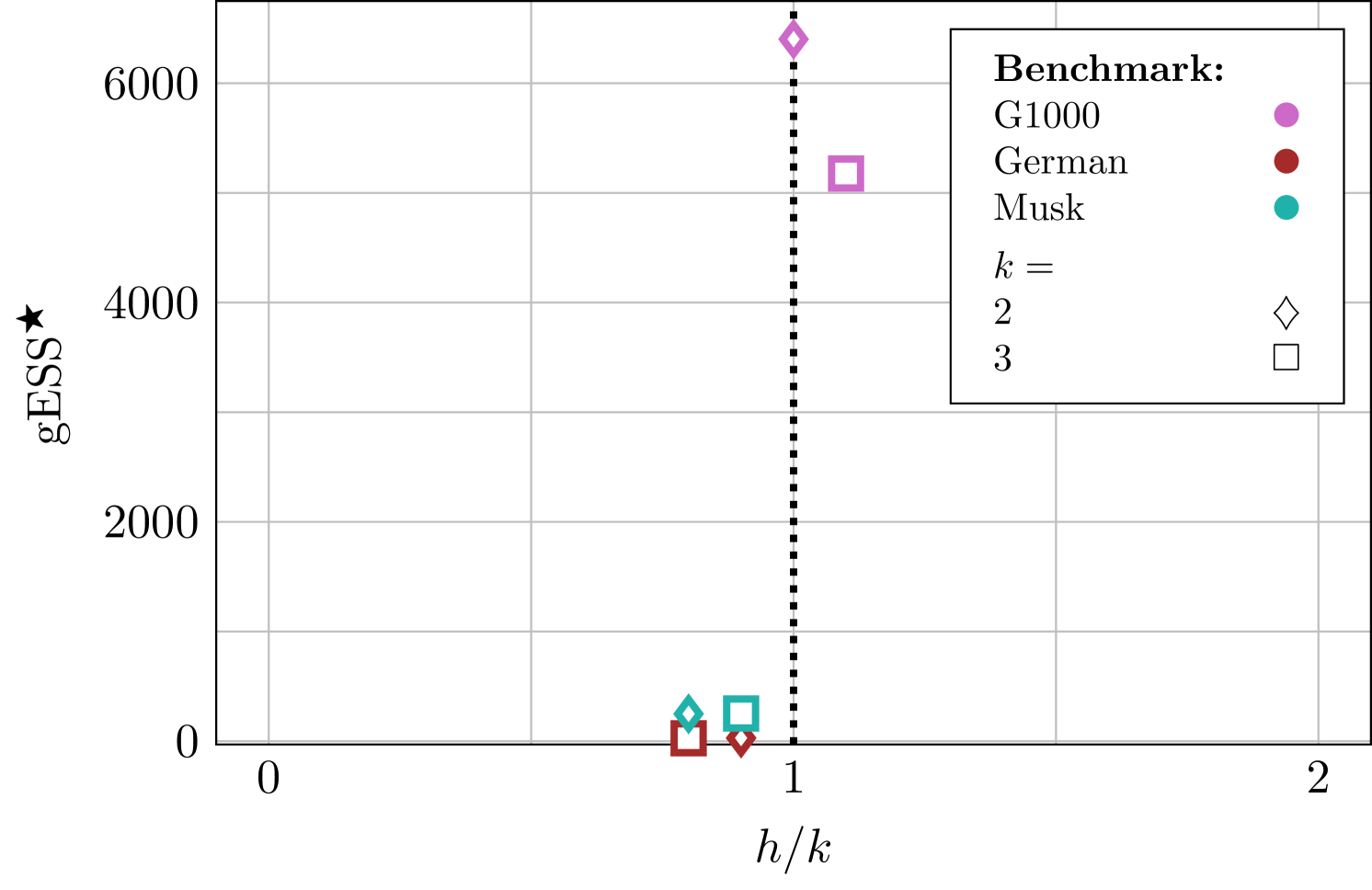
From Table 2, one can observe that top performance is consistently achieved around the CoLSI, , and thus is an obvious candidate for an optimal step size. The deviation of from is not critical at this stage as an optimal step size is to be randomized yet, and only performance at a randomized step matters.
Furthermore, 3-stage integrators always outperform 2-stage ones, as already noticed in [13] and [14]. Hence, it is natural to search for an optimal integrator within the class of 3-stage integrators. Unfortunately, Table 2 does not suggest a unique candidate for the best performed integrator in this class.
We remark that according to [14], BCSS3 and s-AIA3 around CoLSI give rise to very similar accuracy and performance of HMC for all considered benchmarks. For the German benchmark, the efficiencies of all the three 3-stage integrators, i.e. BCSS3, ME3 and s-AIA3, at CoLSI are almost indistinguishable. Thus, it is not surprising that all those integrators appear in Table 2. However, only s-AIA3 adapts its performance to a choice of a step size, and this property becomes important when randomization of a step size is applied. In this context, s-AIA3 looks like the best pick, but this has to be confirmed yet. In the next Sections, we propose a randomization interval for and use the 3-stage integrators (BCSS3, ME3, s-AIA3) and the standard 1-stage Velocity Verlet for its validation.
4 Randomizing optimal step size
Further, we propose an approach for finding an optimal randomization interval for an integration step size (and for its dimensional counterpart ) and compare the resulted HMC performance with the best grad/minESS performance in Table 2.
4.1 Randomization interval
To identify endpoints of a randomization interval for an optimal step size we refer to the upper bound of the expected energy error for 3-stage integrators derived in [14] and plotted for the range of integrators considered in this study in Figure 2.
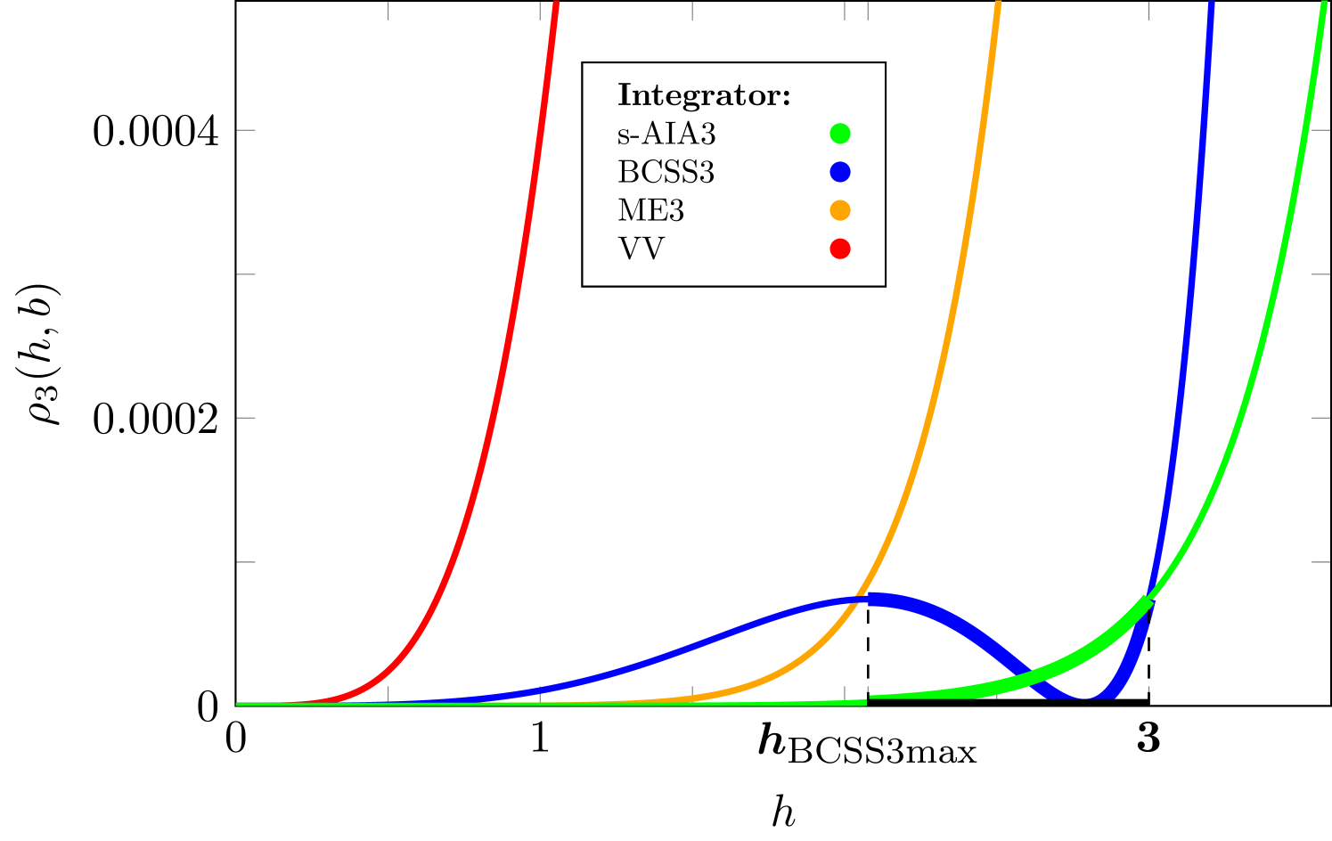
When searching for an optimal randomization interval for the following considerations have to be taken into account. First, the interval should include the step sizes that guarantee the high accuracy of the numerical integration, i.e. . Then, one should keep interval narrow enough to stay close to an estimated optimal value of a step size and to avoid including too small step sizes, which usually satisfy the aforementioned inequality but lead to correlated samples in HMC. Finally, the approximate analysis proposed in [14] may likely result in the overestimated values of the stability limit and thus (see A). This implies a reasonable choice for the right endpoint to be .
On the other hand, we recall that BCSS3 was derived to minimize the maximum of in and thus to achieve the best performance near . The inspection of Figure 2 reveals that with exhibits a local maximum on the left side of . Within the interval (, ) both s-AIA3 and BCSS3 demonstrate very high accuracy, which deteriorates after passing the center of the stability interval. Thus, such an interval obeys all requirements on an optimal randomization interval summarized above.
Therefore, the proposed randomization interval for the nondimensional optimal integration step size is
| (13) |
And the corresponding interval for the dimensional step size is
| (14) |
where and are calculated as proposed in [14] and briefly described in C.
| Benchmark | Sampler | Integrator | |||
|---|---|---|---|---|---|
| G1000 | HMC | s-AIA3 | 1 | ||
| BCSS3 | |||||
| ME3 | |||||
| VV | |||||
| GHMC | s-AIA3 | ||||
| BCSS3 | |||||
| ME3 | |||||
| VV | |||||
| German | HMC | s-AIA3 | 1 | ||
| BCSS3 | |||||
| ME3 | |||||
| VV | |||||
| GHMC | s-AIA3 | ||||
| BCSS3 | |||||
| ME3 | |||||
| VV | |||||
| Musk | HMC | s-AIA3 | 1 | ||
| BCSS3 | |||||
| ME3 | |||||
| VV | |||||
| GHMC | s-AIA3 | ||||
| BCSS3 | |||||
| ME3 | |||||
| VV |
4.2 Validation
To validate the proposed optimal randomized step size and to choose an optimal integrator among the 3-stage integrators, we run HMC simulations with s-AIA3, BCSS3, ME3 and VV at in (14) (in 1-stage units for VV) for all benchmarks introduced in Section 3 and listed in Table 2. The remaining HMC parameters, namely, a number of integration steps per Monte Carlo iteration, , and numbers of burn-in and production iterations, are kept the same as in the numerical experiments in [14]. In addition, we conduct GHMC simulations to evaluate the efficacy of the proposed randomization interval with this sampler in comparison with HMC. For the PMU in Eq. (7), we set to be uniformly selected from the interval (a standard recommendation) and use twice shorter trajectories than for HMC. We remark that this choice of GHMC parameters is based on heuristic intuition. The optimal selection of these parameters are investigated in the following Sections.
The simulation parameters for HMC and GHMC used in this section are summarized in Table 3.
Figure 3 compares performance (in terms of gESS) of HMC and GHMC using and a randomization interval (14) with in Table 2 through /gESS relations.
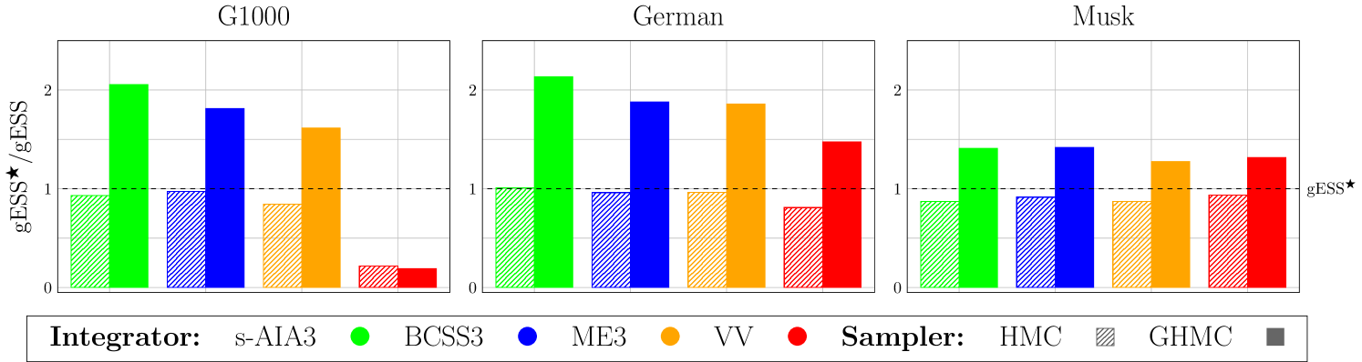
First, we recognize that, as expected, for all benchmarks and for both HMC and GHMC, the adaptive s-AIA3 integrator yields either better or similar sampling performance (in terms of gESS) compared with other tested integrators. Moreover, for GHMC, this performance is visibly higher (up to 2x) than gESS observed in HMC with the newly proposed settings (see Table 3) and with the previously reported setup (Table 2). We notice that the new settings for HMC with s-AIA3 do not necessarily improve the results in Table 2 for each benchmark, but they always stay close to them. We recall that the values in Table 2 for each benchmark were achieved with various integrators and at different step sizes by trial and error, whereas our new settings were generated by the procedure universal for all simulated systems.
In summary, the numerical experiments not only justify the proposed optimal choices for a numerical integrator (s-AIA3), a step size ( / ), and a randomization interval ((13) / (14)), which we will consider for the rest of this study, but also reveal the performance superiority of GHMC over HMC.
We remark that, in contrast to the HMC experiments which relied on the recommended choices of , the results for GHMC in Figure 3 were obtained without a proper tuning of and its additional parameter for the PMU. Obviously, refining these two parameters can further improve performance of GHMC.
Our next objective is to search for optimal, or close to optimal choices of the remaining GHMC parameters.
5 Randomization interval for
We note that GHMC is not a sole HMC-based method which partially refreshes the momenta. The Modified Hamiltonian Monte Carlo, or MHMC, methods for sampling with modified Hamiltonians also rely on the PMU procedure, though the PMU is Metropolized to secure sampling in a modified ensemble [12]. Both GHMC and MHMC use Hamiltonian dynamics for generating proposals but they are accepted more frequently in MHMC due to the better conservation of modified Hamiltonians by symplectic integrators. On the contrary, partially refreshed momentum is always accepted in GHMC, whereas for MHMC, it is accepted according to the modified Metropolis test. Clearly, the MHMC method with very high acceptance rates in the PMU and the GHMC method with very high acceptance rate in the Metropolis test will behave almost indistinguishably.
Here, we aim to derive an optimal parameter for a GHMC method with its optimal settings, i.e. when using the s-AIA3 integrator with (13) or (14). With this in mind, we refer to the procedure proposed in [12] which links in MHMC with the target acceptance rate in the modified Metropolis test in the PMU (see equation (22) in the aforementioned study). Following this idea we express in terms of a step size, parameters of the integrator in use and the target acceptance rate to obtain
| (15) |
Here, is the expected acceptance rate for updated momentum, is the dimension of the system, is the dimensionless counterpart of the integration step size in use, is the coefficient depending on – a number of stages of a numerical integrator – and – the integrator coefficients. In particular [13],
| (16) |
We remark that in the notations of this study corresponds to in [12]. Next, we adapt (15) to the conditions of this work. More precisely, we are interested in optimizing performance of GHMC with s-AIA3 (i.e. ) in . We recall that for s-AIA3, the integrator parameters and are step size dependent and so is .
Given that for GHMC the expected acceptance rates for momentum update are equal to 1, in order to mimic the behavior of (15) in GHMC we set . Therefore, we obtain
| (17) |
where
| (18) |
Moreover, from (7), , which yields
| (19) |
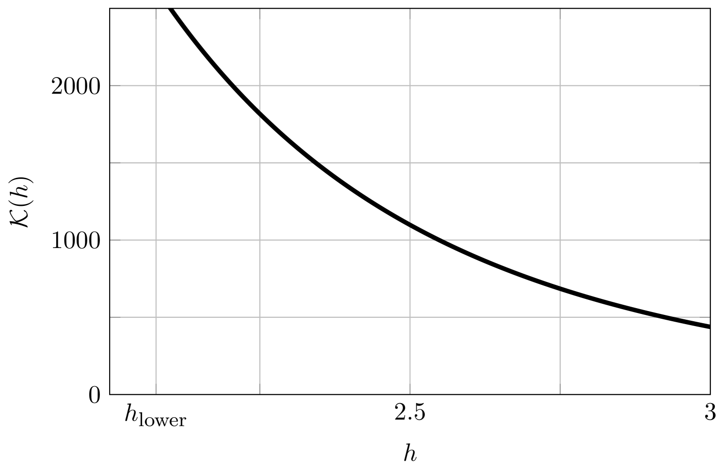
We notice that is a monotonically decreasing function of in the interval (Figure 4), and does not depend on a simulated model. Hence, we can choose the bounds of the randomization interval for optimal as
| (20) |
Thus, an optimal randomization interval for the random noise in the PMU (7) reads as
| (21) |
Optionally, one can adapt (19) in each Monte Carlo iteration for within the randomization interval (13) and its corresponding parameters of s-AIA3. In this case, no additional randomization of is required.
In what follows, we first describe a procedure for an optimal choice of a number of integration steps per Monte Carlo iteration, , and then compare our proposed scheme (21) combined with the various choices of with the commonly recommended and two additional randomization intervals, (close to Metropolized Molecular Dynamics: ) and (close to HMC: ).
6 Optimising Hamiltonian trajectory lengths
A partial momentum update (7) allows for maintaining a favorable direction of sampling, provided (i) the acceptance rate for proposed Hamiltonian trajectories is high and (ii) momentum mixing angle at the PMU is small. Under these conditions, choosing the small possible , i.e. helps to explore in full the area containing a direction once accepted by the Metropolis test, thus mimicking a long but flexible trajectory. So, in contrast to HMC, GHMC may benefit from short Hamiltonian trajectories.
The optimal settings proposed in this study tend to satisfy both conditions, (i) and (ii). Indeed, the randomization interval for optimal step size and the integrator s-AIA3 are chosen to guarantee small expected energy errors(see Figure 2) and hence, high acceptance rates. Furthermore, as follows from (19), , where is the dimension of a simulated system. Thus, the reasonable suggestion for an optimal choice of might be , provided that the underlying analysis for finding an optimal integrator and a step size is accurate.
However, as was indicated in [14], the accuracy of the approach for estimating may suffer when it is applied to systems with clear anharmonic behavior. Such behavior can be caught by inspecting a system-specific value of a fitting factor , which is computed using the simulation data collected at a burn-in stage of a GHMC simulation (see Eqs. (24) and (26) in [14])
| (22) |
where is the highest frequency, is the step size used during the burn-in stage, is the expectation of the energy error, and is the dimension of the system.
Its clear deviation from 1 implies the deviation from harmonic behavior. As a result, for such systems, the expected energy error at the estimated may differ from the one predicted by the analysis of a harmonic oscillator. Moreover, using the expected energy error for 1-stage integrator at for the analysis of 3-stage integrators in [14] leads to an overestimation of , as was discussed in A. Even though, in the settings proposed in this study, it is not only possible to quantify the error introduced by the suggested analysis but also to compensate for it by choosing parameter in the appropriate way.
In particular, let be the expected energy error for 1-stage Velocity Verlet derived at for systems with harmonic behavior () and be the expected energy error for 1-stage Velocity Verlet at an arbitrary for anharmonic systems (). As shown in [14],
| (23) |
We denote
| (24) |
By setting and solving the equation for , one can identify values of that level the difference between the expected errors in a GHMC simulation for harmonic and anharmonic systems. In D, we follow this idea and obtain such values of as a function of . Moreover, taking the suggestion in [19], we randomize so that is the mean of the randomization interval, i.e.
| (25) |
where (see D for details):
| (26) |
The resulting randomization scheme for will be the following:
| (27) |
7 Adaptive Tuning algorithm
Here, we summarize the Adaptive Tuning algorithm (ATune) that, given a simulation system, generates a set of optimal parameters for a GHMC/HMC simulation to give rise to AT-GHMC/AT-HMC.
Similarly to the s-AIA algorithm presented in [14], ATune relies on the simulation data collected during the GHMC/HMC burn-in stage. The latter is run with 1-stage Velocity Verlet using and a simulation step size tuned on the fly, in order to reach a target AR for the burn-in (more details in Appendix B in [14]). Finally, the random noise for the PMU (7) to run the GHMC burn-in stage is selected according to (20)–(21).
On the completion of the GHMC/HMC burn-in stage, the following properties are computed and stored:
-
1.
Acceptance rate (AR)
- 2.
This data is needed for calculation of the fitting factor of the simulated system, which is critical for the nondimensionalization procedure as well as for finding optimal integration coefficients for s-AIA3 integrators and optimal parameters settings for a GHMC/HMC production simulation.
Depending on the availability of frequencies, we consider
| (28) |
where are calculated as described in [14] and summarized in C. Then, the parameters of a s-AIA3 integrator are computed according to the procedure introduced in [14] with the use of the map available in [52].
The GHMC/HMC optimal parameters for the production stage are:
- 1.
- 2.
-
3.
Number of integration steps per Monte Carlo iteration (recommended for GHMC but can be used with HMC)
is chosen following (27).
Finally, the production stage is run using s-AIA3 integrator [14] and the set of optimal parameters for a chosen number of iterations .
The algorithm is outlined in Figure 5.
The ATune algorithm is implemented (with no computational overheads introduced in a production simulation) in the BCAM in-house software package HaiCS (Hamiltonians in Computational Statistics), designed for statistical sampling of high dimensional and complex distributions and parameter estimation in Bayesian models using MCMC and HMC-based methods. A comprehensive overview of the package can be found in [53], whereas applications of HaiCS software are presented in [54, 13, 55, 14].
8 Numerical experiments
The next objective is to numerically justify the efficiency of our new adaptive tuning algorithm using a set of standard benchmarks summarized in Table 4.
8.1 Performance metrics
The irreversibility of GHMC may allow it to reach convergence faster, compared to reversible samplers, like HMC. To check this, we choose the performance metric that includes information about the speed of convergence of the Markov chains. The metric is briefly introduced in Section 3. Here we provide more details on the metric and extend it to the alternative approaches for computing effective sample size (ESS).
Following the recommendation in [50], we consider a chain to be converged if . The Potential Scale Reduction Factor (PSRF) [48] can be calculated as described in [49].
Starting from that, let us define the number of samples in the production chains, required for reaching , as , and evaluate the ratio grad/ESS between the number of gradient computations and ESS for production chains of the length of iterations. Such a metric combines both the information about convergence and sampling efficiency.
The number of gradient evaluations reads as
where is the mean of the number of integration steps per Monte Carlo iteration (it varies depending on a chosen randomization scheme for ) and is the number of stages of an integrator in use (in our case, ). We recall that the number of stages indicates the number of times the algorithm performs an evaluation of gradients per step size. Therefore, represents the theoretical average number of gradient evaluations per Monte Carlo iteration.
In Section 3, we calculate ESS using the effectiveSize function of the coda package of R [51] and consider the minimum ESS across variates, i.e. minESS. We want to include two additional ESS metrics in our list, which now appears like:
-
1.
minESS (coda) – the minimum ESS across variates
-
2.
meanESS (coda) – the average ESS over the sampled variables calculated through the effectiveSize function of the coda package of R [51]
- 3.
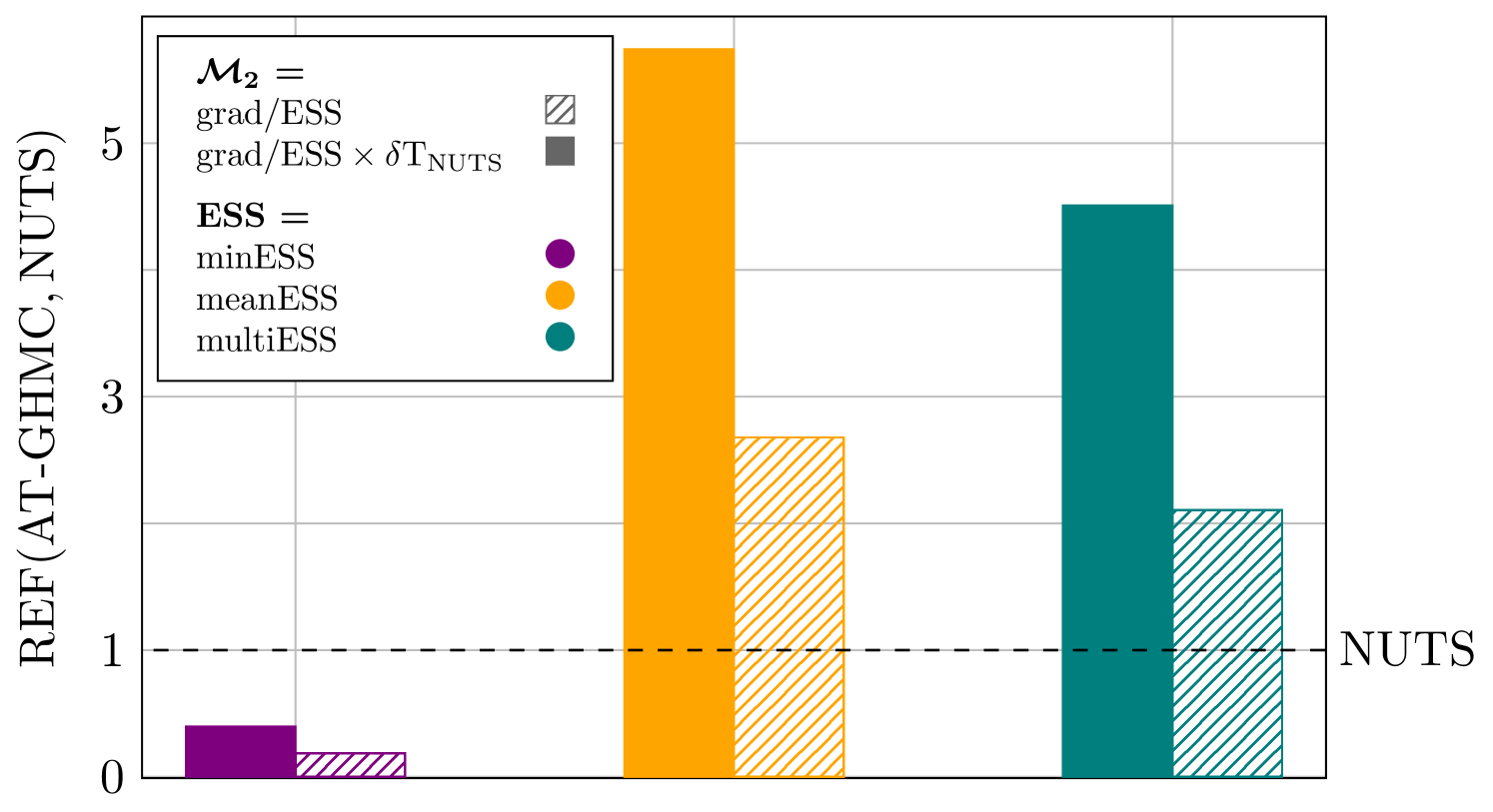
To summarize, we propose three metrics for assessing convergence and sampling performance, such as grad/minESS, grad/meanESS, and grad/multiESS. For each metric, a lower gradient value (grad) indicates better convergence, while a higher ESS suggests improved sampling efficiency. Consequently, the smallest grad/ESS ratio represents the best overall performance.
To enable comparison of efficiency between two samplers, a Relative Efficiency Factor (REF) is introduced as:
| (29) | |||
The REF value quantifies the extent to which outperforms for a particular metric, where ESS is picked from the set {minESS, meanESS, multiESS}.
| Benchmark | Model | Data | (dimension) | (observations) |
| G1000 | [5] | 1000 | - | |
| G500 | 500 | - | ||
| G2000 | 2000 | - | ||
| German | Bayesian Logistic Regression [58] | [59, 20] | 25 | 1000 |
| Musk | [59] | 167 | 476 | |
| Banana [53, 20] | , | 2 | 100 |
8.2 Benchmark tests
We use the the metrics described in 8.1 for the full set of simulation benchmarks (Table 4). For the biggest benchmark (G2000), we consider the ESS metrics evaluated over the first iterations, in order to take into account enough iterations () for the multiESS calculation. We also remark that for Gaussian benchmarks the grad/ESS metrics for the simulations with were calculated over the first ( for G2000), where is the number of iterations required to achieve . The relaxation of the PSRF threshold helped to avoid extremely long simulations () needed for reaching convergence in terms of .
| Benchmark | ||
|---|---|---|
| G1000 | 1 | |
| G500 | 1 | |
| G2000 | 1 | |
| German | 1 | |
| Musk | ||
| Banana |
| Benchmark | ESS | |||||||
| G1000 | minESS | 39373 | 2387 | 1491 | 2509 | 5021 | ||
| meanESS | 0.4596 | 532.1 | 1071 | 2142 | 4285 | |||
| multiESS | 0.3787 | 299.8 | 402.5 | 895.4 | 3069 | |||
| 1 (HMC) | minESS | 132650 | 46712 | 21620 | 11740 | 5554 | ||
| meanESS | 2.530 | 533.6 | 1054 | 2093 | 4198 | |||
| multiESS | 3.712 | 301.3 | 1001 | 2000 | 4001 | |||
| G500 | minESS | 31792 | 1553 | 919.8 | 1090 | 2339 | ||
| meanESS | 0.3429 | 260.0 | 520.7 | 1043 | 2093 | |||
| multiESS | 0.2553 | 170.6 | 320.8 | 384.0 | 1422 | |||
| 1 (HMC) | minESS | 116471 | 42111 | 21821 | 10094 | 4790 | ||
| meanESS | 2.363 | 261.3 | 515.5 | 1035 | 2046 | |||
| multiESS | 3.666 | 107.8 | 321.6 | 563.3 | 1325 | |||
| G2000 | minESS | 63451 | 3305 | 2515 | 5036 | 9195 | ||
| meanESS | 0.6518 | 1104 | 2207 | 4417 | 8853 | |||
| multiESS | 0.5029 | 428.5 | 860.1 | 1723 | 7096 | |||
| 1 (HMC) | minESS | 174435 | 47859 | 22770 | 10870 | 9582 | ||
| meanESS | 2.791 | 1099 | 2178 | 4348 | 8671 | |||
| multiESS | 3.739 | 677.3 | 2000 | 4001 | 8000 | |||
| German | minESS | 1.734 | 13.94 | 25.93 | 53.38 | 113.6 | ||
| meanESS | 0.3463 | 10.15 | 23.84 | 49.05 | 101.0 | |||
| multiESS | 0.1218 | 10.62 | 25.10 | 49.47 | 100.5 | |||
| 1 (HMC) | minESS | 24.92 | 13.25 | 26.18 | 53.09 | 112.6 | ||
| meanESS | 5.860 | 10.56 | 24.45 | 49.23 | 102.9 | |||
| multiESS | 2.334 | 10.88 | 25.44 | 49.44 | 100.8 | |||
| Musk | minESS | 216.8 | 132.3 | 229.4 | 389.7 | 601.3 | 1458 | |
| meanESS | 145.4 | 57.16 | 68.44 | 165.0 | 464.5 | 1031 | ||
| multiESS | 19.79 | 13.58 | 36.00 | 160.4 | 342.0 | 774.5 | ||
| 1 (HMC) | minESS | 6026 | 1476 | 187.7 | 290.3 | 525.7 | 1215 | |
| meanESS | 3068 | 886.8 | 143.5 | 176.3 | 454.6 | 1047 | ||
| multiESS | 375.8 | 93.81 | 50.60 | 159.5 | 279.5 | 506.9 | ||
| Banana | minESS | 287.9 | 247.2 | 167.3 | 168.0 | 158.3 | ||
| meanESS | 190.4 | 167.1 | 141.6 | 167.5 | 156.5 | |||
| multiESS | 202.3 | 165.6 | 151.2 | 183.3 | 169.2 | |||
| 1 (HMC) | minESS | 619.2 | 440.9 | 255.0 | 210.0 | 212.6 | ||
| meanESS | 403.7 | 283.1 | 197.8 | 192.3 | 208.1 | |||
| multiESS | 436.6 | 299.4 | 218.3 | 214.2 | 227.1 | |||
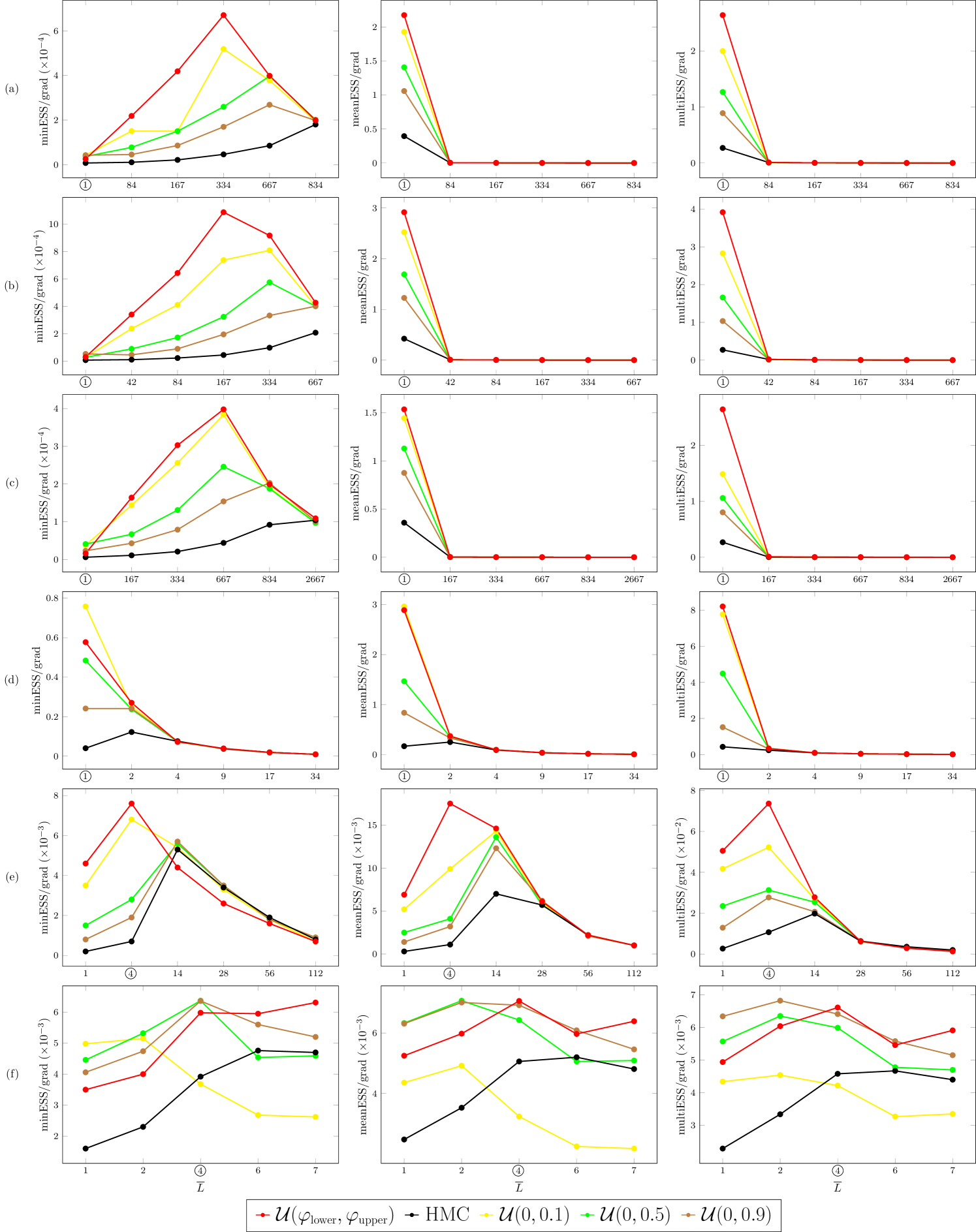
In order to evaluate the optimal settings proposed in this study, we compare our recommended choice (21) with the fixed choice of (which corresponds to standard HMC) and with three randomization intervals , , . For each choice of , in addition to the proposed optimal randomization interval for (27), we consider five different intervals (four for Banana), where the values of are proportional to the dimension of the simulated system. The optimal randomization intervals for and are summarized in Table 5.
As put forward at the end of Section 4.2, we use s-AIA3 as a numerical integrator for Hamiltonian dynamics and the step size randomization interval proposed in Section 4.1 (Eq. (14)).
Table 6 presents the performance comparison between GHMC with and standard HMC () across the tested benchmarks, with varying values of . For any benchmark and for each metric, the best performance is consistently achieved by GHMC (shown in red). Combining GHMC with our proposed choice of leads to the best GHMC results for the average metrics, i.e. grad/meanESS and grad/multiESS. Moreover, for non-Gaussian benchmarks (also, with smaller dimensions), grad/minESS shows the best results with such a choice of . For Gaussian benchmarks, the best results for grad/minESS are reached for larger values of – they are lower for GHMC (around ) and higher for HMC ().
The results obtained with other tested randomization intervals for , , , , support our choice for the optimal randomization interval (, ) and can be examined in E.
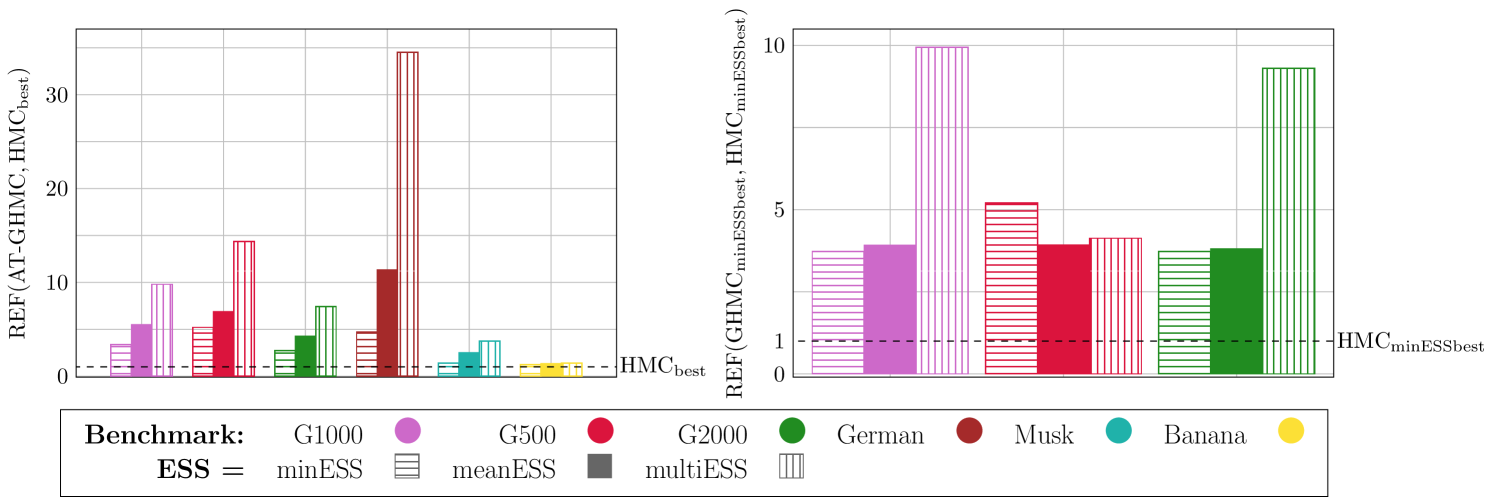
On the right: Relative efficiency (REF (29)) of GHMC with respect to HMC with their best settings for minESS (see Table 6) for the Gaussian benchmarks – G1000, G500, G2000. All the benchmarks show the superiority (up to 10x) of GHMC over HMC with each performance metric.
Finally, in Figure 6, we provide performance comparison in terms of the REF (29) between GHMC with our optimal settings, i.e. AT-GHMC, and HMC with its best settings found heuristically (see Table 6) using all proposed ESS metrics and all tested benchmarks. For the Gaussian benchmarks, we also present the comparison at the values that optimize the minESS metric in HMC and GHMC (see Table 6). Both plots in Figure 6 confirm the improvements (up to 34x and 10x, respectively) gained with our proposed GHMC settings across all metrics and benchmarks. They also demonstrate that greater improvements are achieved with the average metrics, i.e. meanESS and multiESS.
9 Applications – Case studies
Next, we apply ATune to three case studies:
-
1.
Patient resistance to endocrine therapy in breast cancer
-
2.
Cell-cell adhesion dynamics
-
3.
Influenza A (H1N1) epidemics outbreak.
9.1 Patient resistance to endocrine therapy in breast cancer
Estrogen-positive (ER+) breast cancer is the most common subtype of breast cancer, accounting for over 70% of all breast tumors diagnosed. Hormone therapies such as tamoxifen are the gold-standard treatment. However, a significant amount of patients develops resistance to the treatment, which constitutes a serious clinical problem. The development of this resistance is not yet well understood, and plenty of clinical and laboratory research aims to find which genes may be relevant to the problem.
For one such clinical study presented in [60], ER+ breast cancer patients treated with tamoxifen for 5 years were tested for the presence of a specific gene marker, SOX2. The objective of the study was to analyze the connection between SOX2 and the emergence of resistance to tamoxifen treatment. An overexpression of this gene was previously identified in bioinformatic analyses of resistant breast cancer cells as a key contributor for resistance, but clinical evidence was presented in [60] for the first time.
The dataset used in our work stems from that clinical trial. It contains numerical data for SOX2 values and 7 other gene-related covariates taken from 75 tumors samples. The recorded response variable was the event of relapse after 5 years. Notably, the SOX2 variable perfectly separates the dataset for this response variable, as all cases with SOX2 values below 3 respond well to the treatment and all those above this value present a resistant response. The appearance of separation implies that maximum likelihood estimates do not exist for some binary classification models such as logistic regression [61] in the classical frequentist interpretation. The perfect separation makes the Bayesian framework natural to model such a dataset, as it can provide estimates for the parameters involved without the need to use regularization techniques.
The model of choice is a Bayesian Logistic Regression, where the dataset has 75 observations and dimension (including intercept parameter). We test the effect of three priors, informative , weakly informative (according to [62]) and low informative .
We compare the performance of AT-GHMC proposed in this study against the No-U-Turn-Sampler (NUTS) [5], the optimized HMC sampler implemented in Stan [63] using its R interface rstan [64]. NUTS in Stan uses the leapfrog/Verlet integrator [6] and the original optimization routine to determine both a step size, , and a number of Hamiltonian dynamics integration steps per iterations, . Additionally, we perform numerical experiments with HMC using from Eq. (27) (AT-HMC) and setting (HMC). The latter is determined such that the integration leg matches that found by NUTS.
All samplers are run with the same number of burn-in iterations, , to ensure a fair comparison. We assess performance using grad/ESS metrics introduced in Section 8.1. Small values of in NUTS are expected, given its optimization routine aims to bring PSRF close to 1. The simulation settings are summarized in Table 7.
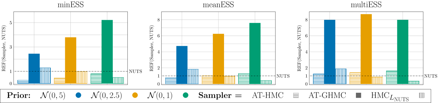
Figure 7 compares the sampling performance of AT-GHMC, AT-HMC, and HMC with NUTS using REF metrics (29) for . AT-GHMC consistently outperforms NUTS across all metrics and priors, achieving more than 8 times improvement (e.g., multiESS for the prior).
| Prior | Sampler | ||||
|---|---|---|---|---|---|
| AT-GHMC | 300 | 1 | |||
| AT-HMC | 200 | 1 | - | ||
| HMC | 100 | - | |||
| NUTS | 100 | - | |||
| AT-GHMC | 100 | 1 | |||
| AT-HMC | 100 | 1 | - | ||
| HMC | 200 | - | |||
| NUTS | 100 | - | |||
| AT-GHMC | 100 | 1 | |||
| AT-HMC | 200 | 1 | - | ||
| HMC | 200 | - | |||
| NUTS | 100 | - |
We emphasize that, the ATune algorithm does not offer an optimal choice of for HMC. The values of (27) used in AT-HMC are the recommended values for GHMC. However, the strong meanESS and multiESS performance of AT-HMC in all experiments confirms their applicability in HMC. On the other hand, the relative efficiency of HMC with respect to NUTS shows its strong dependence on a chosen prior. Specifically, HMC demonstrates visible improvements over NUTS with the low informative prior ; the comparable performance with NUTS if the chosen prior is , and the poor sampling efficiency with the highly informative prior . For , the improved performance can be attributed to the higher accuracy and longer optimal step size of the 3-stage integrator (s-AIA3) employed in HMC compared to those achievable with the standard 1-stage Verlet integrator used in NUTS. On the contrary, the poor performance of HMC with is likely caused by the underestimation of hinted by the comparison of its value with (see Table 7). Indeed, the values are close, which is not what one expects when comparing optimal step sizes for 1- and 3- stage integrators. It is also not the case for and , where optimal step sizes are longer than the NUTS optimal step sizes (less pronounced for though), and where AT-GHMC and AT-HMC have never been outperformed by NUTS. These observations are encouraging. They mean that even in the worst scenario, when the estimated optimal parameters are less accurate, they still guarantee the good sampling performance (see AT-GHMC and AT-HMC for and are not inferior to the optimal parameters offered by the state-of-the-art NUTS approach. Moreover, the sampling advantages of GHMC over HMC, enhanced by the stochastic procedure for finding its optimal settings, disregard the inaccuracy in the estimation of an optimal step size and, as a result, AT-GHMC demonstrates a significant improvement over NUTS, AT-HMC and HMC as happened in the case of . The fact that the performance of AT-HMC in this case is comparable with, or better than the NUTS performance also confirms the robustness of the proposed methodology.
9.2 Parameter inference on a cell-cell adhesion model
Many phenomena on the cellular level such as tissue formation or cell sorting can be explained by introducing differential cell-cell adhesion [65, 66, 67, 68, 69, 70]. This phenomena has been used to explain pattern formation for zebrafish lateral lines [71, 72], cancer invasion modeling [66], and cell sorting in early fly brain [70] and early mice brain development [73]. When modeling such biological systems using PDEs, the adhesion can be represented by means of a non-local interaction potential [66, 65, 68, 69]. To enhance predictive power of such models, a careful calibration of the model parameters according to experimental lab data is required. This task can become increasingly difficult due to sparsity of available data or increasing complexity of the model (such as, for example, by the addition of an interaction term). The application of state-of-the-art methodologies for performing parameter estimation on PDE models is receiving lots of attention in the last years [74, 75, 76], and, in this context, our goal is to investigate the feasibility of using the methodology introduced in this work for the task.
To achieve this goal, we propose a benchmark PDE model:
| (30) |
which describes the time evolution of the density of cells , ( is the spatial dimension), as governed by a series of potentials. In (30), is a density of the internal energy and is an interaction potential (also called an interaction kernel) describing cell adhesion. The convolution () gives rise to non-local interactions. Depending on the explicit form of the potentials, they can describe a wide range of biological phenomena such as the formation of ligands through long philopodia, modeled by nonlocal attractive potentials, and volume constraints, modeled by strong repulsive nonlocal potentials or nonlinear diffusive terms. We refer to [77] for more information about the applications of these aggregation-diffusion models in the sciences. We consider the following explicit forms for and :
| (31) |
where gives rise to a diffusion term, governed by the diffusion exponent . In the limit , one recovers linear diffusion, whereas if the term represents porous medium and leads to finite speed propagation fronts. The diffusion coefficient defines the cell mobility in the medium. On the other hand, the explicit form of leads to symmetric attraction between cells due to ligands formation on the cell’s membrane. The strength of the attraction is given by the parameter , whereas controls the range of the interaction.
Our purpose is to perform Bayesian inference of the parameters of this model using three different MCMC methods, and to evaluate the efficiency of each tested sampler for this class of models. Parameter inference in a Bayesian framework requires sampling from the posterior distribution of parameters given by , where are the experimental data and is the vector of model parameters. For the proposed model, the data consists of a collection of measurements of the cell density at different spacial points and different times . In cell modeling, it is usual to assume that the experimental data stems from the proposed model with additive Gaussian noise , i.e. . Under this assumption, the likelihood takes the form:
| (32) |
In this work, we use synthetic data generated from model (30) in a one dimensional case (). First, we numerically solve the model in the interval by using the finite volume scheme proposed in [78, 79] with a spacial meshing of 50 cells and a time step of , resulting in a total of 51 time points. We denote the numerical solution at point and time as . We then generate the synthetic data by adding Gaussian white noise to each cell and time point , where is the noise parameter.
We consider two different variations of the model for the numerical experiments. In the first one (3-parameter model) the parameters sampled are the diffusion coefficient , the diffusion exponent from the internal energy potential in (LABEL:eq:pdemodel_potentials), and the model independent noise parameter . The remaining parameters in (LABEL:eq:pdemodel_potentials) are fixed to and . In the second variation (4-parameter model), we extend the previous model to also consider as a sampled parameter, leaving as the only fixed parameter in (LABEL:eq:pdemodel_potentials). The chosen priors are , , , and .
Three sampling methodologies are examined: Random Walk Metropolis-Hastings (RW) (the most commonly used method for Bayesian inference), AT-HMC and AT-GHMC. We evaluate performance using the metrics introduced in Section 8.1. For this study, the metrics are computed over the first iterations, where is the number of iterations needed for convergence. We note that the slower-converging RW requires a large number of iterations to meet the strict threshold (). Therefore, for this sampler, we relax a convergence threshold to 1.1, as suggested in [48]. Since RW does not involve gradient evaluations (which constitute the bulk of the computational cost in HMC/GHMC), we normalize ESS metrics with respect to the simulation time T.
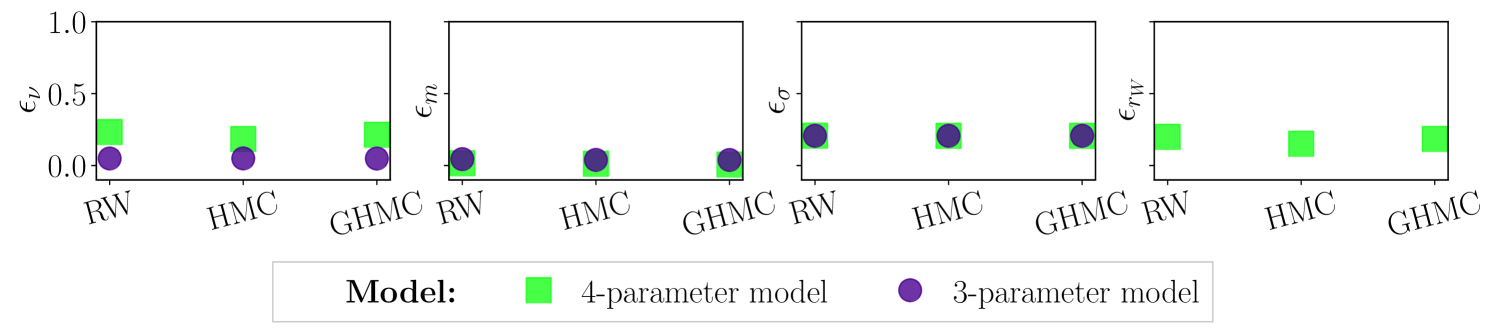
Figure 8 shows the relative error for each parameter and both models, defined as , where is the true parameter value used for generating the synthetic data and is the mean parameter value obtained from the RW, AT-HMC and AT-GHMC simulations considering the first 5000 iterations after convergence. The three samplers are able to recover the true parameter values with high precision, as evidenced by the low relative errors, meaning all parameter can be confidently identified with small variance. In particular, GHMC and HMC exhibit higher precision than RW. Nevertheless, the number of iterations needed to reach the stationary distribution are vastly different across samplers: AT-GHMC needs samples to converge for both models, whilst AT-HMC requires and RW (even with the relaxed convergence threshold), confirming that AT-GHMC has a much faster convergence rate.
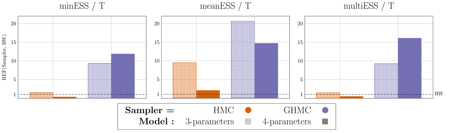
In Figure 9, we present the comparison of the REF metric (29) for the three samplers (Sampler1 = {AT-GHMC, AT-HMC}, Sampler2 = RW) for both models, in terms of ESS/T, . AT-GHMC exhibits high efficiency across all metrics and models, outperforming the popular RW and AT-HMC by up to an order of magnitude in both models. Additionally, AT-GHMC shows visibly higher relative performance in the 4-parameter model than in the 3-parameter model for two out of three considered metrics. This may indicate the potential of the method for high dimensional problems. These results suggest that AT-GHMC provides a suitable framework for PDE calibration. On the other hand, AT-HMC displays worse performance than RW in two out of three metrics when increasing the dimension of the model. Most likely, an optimal choice of for GHMC (27) does not necessarily translate to optimal performance for HMC, especially for higher dimensions.
9.3 Influenza A (H1N1) epidemics outbreak
Mechanistic disease transmission models are mathematical frameworks used to describe how infectious diseases spread through populations. These models commonly employ compartmental structures that classify individuals into distinct states (such as susceptible, infected, recovered), and define transitions between these states over time using systems of ordinary differential equations (ODEs). Classical disease transmission models are often deterministic, meaning that the system’s evolution is fully determined by its parameters and initial conditions, always yielding the same outcome for a given setup. While deterministic models offer valuable insights into average system behavior, they fail to capture the inherent variability and stochasticity of real-world disease transmission. To address this limitation, mechanistic models can be enriched with statistical components that incorporate observational data to infer the underlying parameters. This is achieved by overlaying a probabilistic (or generative) model onto the deterministic structure. Bayesian inference, in particular, has proven highly effective for this purpose (refer to [80, 55] and references therein).
As an illustrative example, we consider an outbreak of influenza A (H1N1) in 1978 at a British boarding school involving 763 students. The dataset, available in the R package outbreaks [81], records the daily number of students confined to bed over a 14-day period. Following [80], we model the outbreak dynamics using a classical SIR (Susceptible-Infected-Recovered) model [82], coupled with a negative binomial observation model to account for overdispersion in the reported case counts. The model includes the transmission rate, , and the recovery rate, , which govern the transitions from susceptible to infected and from infected to recovered, respectively. For the prior distributions, we assume and , where denotes a normal distribution truncated at . The prior specification is completed by assigning an exponential prior to the inverse of the dispersion parameter, , of the negative binomial distribution, i.e. . The initial conditions are set as , , and thus .
| Sampler | ||||
|---|---|---|---|---|
| AT-GHMC | 2250 | |||
| NUTS | 140 | - |
As in Section 9.1, we compare the performance of two samplers: AT-GHMC and NUTS [5], as implemented in the R package rstan [64]. We note that, in both cases, the (approximate) solution to the ODE system is obtained using the CVODES component of the SUNDIALS suite [83]. Specifically, we use the ODE solver that relies on the backward differentiation formula (BDF) method. Similarly to the breast cancer study, both samplers are run with the same number of burn-in iterations, and their performance is assessed in terms of the grad/ESS metrics calculated over the first iterations after the burn-in (see Section 8.1).
The simulations settings for the numerical experiments are summarized in Table 8. Figure 10 shows the relative efficiency REF (29) of AT-GHMC over NUTS, evaluated in terms of grad/ESS, . In addition, to account for the extra computational cost incurred solely by NUTS due to its optimization process during the burn-in phase, we multiply the grad/ESS metrics for NUTS by a factor quantifying such overheads, . This factor is carefully evaluated using the rstan package.
AT-GHMC with our proposed settings outperforms NUTS in terms of both meanESS and multiESS, with improvements increasing from a factor of 2x when no NUTS computational overheads are considered to 5x otherwise. In contrast, NUTS achieves faster convergence and better sampling with the most restrictive metric, minESS, which is likely enabled by the use of a tuned mass matrix. This trend aligns with the findings from the breast cancer study (Figure 7), where AT-GHMC shows more significant improvements over NUTS for average ESS metrics than for minESS. This suggests that tuning a position-dependent mass matrix during the NUTS burn-in stage may have a pronounced effect on the efficiency of an HMC algorithm in sampling complex distributions. Nevertheless, the computational time analysis shows that, in this case study, NUTS requires approximately twice the computational time of a tuned GHMC to achieve on average twice lower sampling performance, as highlighted in Figure 10.
10 Conclusion
The challenge of tuning appropriate hyperparameters to enhance HMC sampling performance has been extensively addressed by the statistical community. In contrast, GHMC, despite its promising potential to improve sampling efficiency due to the inherent irreversibility of its Markov chains, has not garnered comparable attention.
Here we present a computationally inexpensive adaptive tuning approach ATune which generates optimal parameters settings on the fly for HMC and GHMC simulations, bringing forth adaptively tuned AT-HMC and AT-GHMC methods. Given a simulated system, the new methodology delivers a set of system-specific optimized HMC/GHMC hyperparameters, without introducing any additional computational overhead during the production simulation stage.
To determine an optimal integration step size, we build on the insights from the s-AIA adaptive integration approach introduced in [14]. We propose a system-specific randomization interval that minimizes energy error near the center of an estimated stability interval – the region typically associated with the most efficient performance [10, 42]. Additionally, we confirm that the s-AIA3 integrator consistently outperforms fixed-parameter integrators when combined with both HMC and GHMC samplers. We notice that even following the general recommendations for GHMC settings leads to its superior performance over manually tuned HMC. These findings motivate a deeper exploration of the proper tuning of and parameters for GHMC.
Leveraging the methodology proposed in [12], we develop an automated procedure for finding an optimal value for the random noise parameter in PMU (7), based solely on the size of the simulated system (assuming the simulation step size and numerical integrator are chosen as discussed). When applied to high-dimensional systems, this approach leads to smaller modifications of momentum, which, combined with the high accuracy provided by s-AIA3 and an optimal choice of , facilitates the use of shorter trajectories, thus enhancing sampling efficiency in GHMC [37]. We note that, unlike the optimization procedures proposed for other hyperparameters, the selection of the optimal random noise can be performed prior a burn-in stage, relying only on the known dimensionality of the system. As a result, we propose employing the optimal from the very start of a GHMC simulation, rather than limiting it to the production stage only.
The introduced optimal hyperparameter settings exhibit superiority over other combinations of hyperparameters, leading to significant GHMC performance improvement across a set of popular benchmarks. Additionally, the performance gains observed when comparing our results to state-of-the-art samplers in three distinct real-world case studies indicate the broad applicability and effectiveness of AT-GHMC for diverse probabilistic models. It is worth noting that, although the optimal choice of is specifically tailored for GHMC, also enhances sampling efficiency when applied to HMC in some cases, especially of small dimensions.
The proposed ATune algorithm can be easily implemented in any software package for statistical modeling using Bayesian inference with Hamiltonian Monte Carlo to offer the advantages of AT-GHMC over conventional HMC.
Appendix A Overestimation of a dimensional stability interval for 3-stage integrators
A.1 Overestimation of the expected acceptance rate in the s-AIA analysis
We consider the high-dimensional asymptotic formula for expected acceptance rate [3] proven for Gaussian distributions in a general scenario [84], i.e.
| (33) |
with and
| (34) |
Replacing (33) with its asymptotic expression
| (35) |
allows us to compute as proposed in [14]:
| (36) |
Here, is the acceptance probability of the Metropolis test. This gives rise to the system-specific fitting factor (see C) and a system-specific (for more details see [14]). In particular, we have
that brings to
| (37) |
The impact of the approximation error in (34) on the estimated can be evaluated by substituting the RHS of the equation (34) into the inequality which holds by definition. Then, one obtains:
| (38) |
For , as in our case, the inequality (38) becomes
Therefore, the expected acceptance rate in (35) overestimates the real expected acceptance rate, leading to the underestimation of the energy error in (36), which in turn, results in the overestimation of in (37). We notice, however, that such an error is small due to the functional dependencies between the variables involved in the estimation of and the condition , though the order of such an approximation is out of the scope of this study.
A.2 Overestimation of for 3-stage integrators
A closed-form expression for the expected energy error produced by 1-stage Velocity Verlet with = 1 in the case of a univariate Gaussian model, was derived in [14]:
| (39) |
where is the nondimensional counterpart of the integrations step size (see [14] and C).
Eq. (39) comes from the more general expression for the expected energy error for a univariate Gaussian model [10]
| (40) |
Here, are coefficients depending on an integrator in use, and is the nondimensional counterpart of a given dimensional simulation step size (see C).
It is also possible to derive from (40) similar expressions for the 2- and 3-stage cases (see A.3 and [14], respectively).
In particular,
- 1.
- 2.
One can immediately notice that, contrary to the formula (39) for the standard 1-stage Velocity Verlet, both (41) and (42) do not allow for closed-form expressions for , which are needed for estimating stability intervals with the procedure proposed in [14].
However, some analysis and comparison of in (41)–(42) with in (39) is possible. For that, we first apply a change of variables , and , where in (39), (41) and (42), respectively.
Afterwards, we can equate both (41) and (42) to in (39) and see which values of solve the equation.
-
1.
: by equating (41) with and (39) with , one obtains
which brings to
(43) with two nonnegative roots, , , or, equivalently, , in (41). Thus, Eq. (39) and Eq. (41) coincide at the CoLSI. Hence, we can conclude that the analysis made with (39) as proposed in [14] is reliable for the estimation of a dimensional stability limit for a 2-stage integrator.
-
2.
: by equating (42) with and (39) with , one gets
leading to
(44) (44) has 3 nonnegative roots , and . However, , i.e. is not a root of (44). The closest to CoLSI is . Clearly, the analysis carried out using (39) brings to an overestimation of a stability interval for 3-stage integrators and may not find an accurate estimation of a dimensional stability limit or CoLSI for a 3-stage integrator. We have to remark that the calculation of dimensional does not solely depend on but also on the simulated properties, such as AR, extracted at the HMC burn-in stage. Obviously, acceptance rates obtained with 1- and 3-stage integrators should differ, and thus it is not feasible to make an accurate prediction of the estimation error for within the proposed analysis. In any case, using the randomization interval suggested in (13) resolves this problem by probing the step sizes smaller or equal than , including .
A.3 Calculation of 2-stage Velocity Verlet integration coefficients
Consider the harmonic oscillator with Hamiltonian
| (45) |
and equations of motions
| (46) |
A 2-stage palindromic splitting integrator ( is the integration step size) acts on a configuration at the -th iteration as
| (47) |
for suitable method-dependent coefficients , , , .
Appendix B Local maximum of for
Appendix C map for a simulation step size
Following the nondimensionalization approaches presented in [14], here we derive a map which, given a dimensionless step size , computes its dimensional counterpart .
s-AIA [14] uses a multivariate Gaussian model and simulation data obtained at the HMC burn-in stage to compute a system-specific fitting factor . Fitting factors quantify the step size limitations imposed by nonlinear stability in numerical schemes employed for the integration of the Hamiltonian dynamics. These factors (also called safety factors (SF) in [11]) are closely related to stability limits on products of frequencies and step sizes introduced for up to the 6th order resonances for applications in molecular simulations in [85]. Those limitations are usually related to the frequency of the fastest oscillation , and provide a nondimensionalization map for a simulation step size , i.e.
| (50) |
In [14], Sec. 4, we introduced three optional nondimensionalization maps with different levels of accuracy and computational effort. First, we distinguish between the more demanding and accurate , which requires the computation of the frequencies of the harmonic forces [14], and the cheaper and less precise (see Eq. (28)), where
| (51) |
Here, is the integration step size used during the HMC burn-in simulation, AR is the acceptance rate observed in such a simulation, and is the dimension of the simulated system.
On the other hand, if the system frequencies are available, the nondimensionalization approach adapts according to the standard deviation of their distribution. More explicitly, if the distribution of the frequencies is disperse (), we apply a correction to (50), and define a nondimensionalization factor
| (52) |
to replace in (50). Otherwise, if , the nondimensionalization factor reads
| (53) |
where is defined as in (28).
In any case, given a nondimensional step size , its dimensional counterpart for a specific simulated system is computed as
Appendix D calculation
As proposed in Section 6, we consider
where represents the expected energy error for 1-stage Velocity Verlet at an arbitrary for anharmonic systems (), and (23) stands for the expected energy error for 1-stage Velocity Verlet derived at for systems with harmonic behavior (). is the fitting factor defined in (22).
One can express the quantity as
where
Therefore, the resulting expression for is
| (54) |
Here, is a coefficient that depends on the specific integrator in use (see [10]). In particular, it is determined by the number of stages in the integrator, the integration coefficients, and the step size.
We recall that is a free parameter. Then, to minimize the difference between and (as suggested in Section 6) one can find such a value of that . Thus, using Eq. (54), one obtains
| (55) |
In Section 6, we argue that an optimal value of for GHMC in the proposed settings should be small. Therefore, we take in (55), which simplifies to
| (56) |
Combining and equation (56) yields . However, by definition, . Therefore, and . This suggests a choice of for the systems with harmonic behavior, i.e. with .
On the other hand, as discussed in A, is overestimated for sAIA3 by a factor of . Consequently, it is reasonable to consider for the systems with . In practice, it might be reasonable to relax condition on and choose for systems with rounded up to 1, i.e. .
Otherwise (i.e. if ), we refer again to Eq. (55) and set . This leads to
In the settings of this study, the integration step size is drawn from (see Section 4.1). We therefore calculate (as detailed in [10] and Appendix A in [14]) at the midpoint , which gives . Thus, we obtain
Appendix E Sampling Performance of GHMC with different choices of and
Figure E.1 presents the comparison of ESS/grad metric, ESS ={minESS, meanESS, multiESS}, obtained for the tested benchmarks using GHMC with different randomization schemes for and , and the optimal randomization scheme for the integration step size (Section 4). The s-AIA3 integrator is used in all experiments.
Figures E.1(a)–E.1(c) illustrate that, for the Gaussian benchmarks, ensures the best (or close to the best) results for minESS/grad metric among the ones obtained with all the tested randomization schemes, regardless of the choice of .
For the average metrics meanESS and multiESS, a significant improvement with is observed only at the optimal (indicated by a circle). With longer trajectories, GHMC with any tested choice of , including , i.e. HMC, exhibits reduced performance in terms of meanESS and multiESS.
The results for the BLR benchmarks, German and Musk, are displayed in Figures E.1(d) and E.1(e), respectively. For the German benchmark (Figure E.1(d)), the randomization scheme for slightly outperforms our optimal setting in terms of the minESS/grad metric and performs comparably to our approach on the average metrics. In contrast, for the Musk benchmark (Figure E.1(e)), our method achieves the highest values across all ESS metrics, demonstrating superior performance.
For the Banana benchmark (Figure E.1(f)), the proposed optimal settings for , and lead either to the best or close to the best performance with all tested metrics.
Acknowledgments
We gratefully acknowledge Caetano Souto Maior for his valuable contributions at the early stages of this study, particularly to the implementation of the cell-cell adhesion PDE model in HaiCS.
This research was supported by MICIU/AEI/10.13039/501100011033 and by ERDF A way for Europe under Grant PID2022-136585NB-C22; by the Basque Government through ELKARTEK Programme under Grants KK-2024/00062, and through the BERC 2022-2025 program. We acknowledge the financial support by the Ministry of Science and Innovation through BCAM Severo Ochoa accreditation CEX2021-001142-S / MICIU/ AEI / 10.13039/501100011033 and PLAN COMPLEMENTARIO MATERIALES AVANZADOS 2022-2025, PROYECTO 1101288. The authors acknowledge the financial support received from the grant BCAM-IKUR, funded by the Basque Government by the IKUR Strategy and by the European Union NextGenerationEU/PRTR. JAC was supported by the Advanced Grant Nonlocal-CPD (Nonlocal PDEs for Complex Particle Dynamics: Phase Transitions, Patterns and Synchronization) of the European Research Council Executive Agency (ERC) under the European Union’s Horizon 2020 research and innovation programme (grant agreement No. 883363). M.X. R-A was partially funded by the Spanish State Research Agency through the Ramón y Cajal grant RYC2019-027534-I. This work has been possible thanks to the support of the computing infrastructure of the BCAM in-house cluster Hipatia, i2BASQUE academic network, Barcelona Supercomputing Center (RES, QHS-2025-1-0027), DIPC Computer Center and the technical and human support provided by IZO-SGI SGIker of UPV/EHU.
References
- [1] S. Duane, A. Kennedy, B. J. Pendleton, D. Roweth, Hybrid Monte Carlo, Physics Letters B 195 (2) (1987) 216–222. doi:https://doi.org/10.1016/0370-2693(87)91197-X.
- [2] R. M. Neal, MCMC using Hamiltonian dynamics, Handbook of Markov Chain Monte Carlo 2 (11) (2011) 2. doi:10.1201/b10905-6.
-
[3]
A. Beskos, N. Pillai, G. Roberts, J. M. Sanz-Serna, A. Stuart,
Optimal tuning of the hybrid
Monte Carlo algorithm, Bernoulli 19 (5A) (2013) 1501–1534.
URL http://www.jstor.org/stable/42919328 - [4] M. Betancourt, S. Byrne, M. Girolami, Optimizing The Integrator Step Size for Hamiltonian Monte Carlo, arXiv preprint, arXiv:1411.6669 (2014). doi:10.48550/arXiv.1411.6669.
-
[5]
M. D. Hoffman, A. Gelman,
The
No-U-Turn sampler: adaptively setting path lengths in Hamiltonian
Monte Carlo., Journal of Machine Learning Research 15 (1) (2014)
1593–1623.
URL https://www.jmlr.org/papers/volume15/hoffman14a/hoffman14a.pdf - [6] L. Verlet, Computer "Experiments" on Classical Fluids. I. Thermodynamical Properties of Lennard-Jones Molecules, Physical Review 159 (1967) 98–103. doi:10.1103/PhysRev.159.98.
- [7] W. C. Swope, H. C. Andersen, P. H. Berens, K. R. Wilson, A computer simulation method for the calculation of equilibrium constants for the formation of physical clusters of molecules: Application to small water clusters, The Journal of Chemical Physics 76 (1) (1982) 637–649. doi:10.1063/1.442716.
- [8] R. I. McLachlan, On the Numerical Integration of Ordinary Differential Equations by Symmetric Composition Methods, SIAM Journal on Scientific Computing 16 (1) (1995) 151–168. doi:10.1137/0916010.
- [9] T. Takaishi, P. de Forcrand, Testing and tuning symplectic integrators for the hybrid Monte Carlo algorithm in lattice QCD, Physical Review E 73 (2006) 036706. doi:10.1103/PhysRevE.73.036706.
- [10] S. Blanes, F. Casas, J. M. Sanz-Serna, Numerical integrators for the Hybrid Monte Carlo method, SIAM Journal on Scientific Computing 36 (4) (2014) A1556–A1580. doi:10.1137/130932740.
- [11] M. Fernández-Pendás, E. Akhmatskaya, J. M. Sanz-Serna, Adaptive multi-stage integrators for optimal energy conservation in molecular simulations, Journal of Computational Physics 327 (2016) 434–449. doi:10.1016/j.jcp.2016.09.035.
- [12] E. Akhmatskaya, M. Fernández-Pendás, T. Radivojević, J. M. Sanz-Serna, Adaptive Splitting Integrators for Enhancing Sampling Efficiency of Modified Hamiltonian Monte Carlo Methods in Molecular Simulation, Langmuir 33 (42) (2017) 11530–11542, pMID: 28689416. doi:10.1021/acs.langmuir.7b01372.
- [13] T. Radivojević, M. Fernández-Pendás, J. M. Sanz-Serna, E. Akhmatskaya, Multi-stage splitting integrators for sampling with modified Hamiltonian Monte Carlo methods, Journal of Computational Physics 373 (2018) 900–916. doi:10.1016/j.jcp.2018.07.023.
- [14] L. Nagar, M. Fernández-Pendás, J. M. Sanz-Serna, E. Akhmatskaya, Adaptive multi-stage integration schemes for Hamiltonian Monte Carlo, Journal of Computational Physics 502 (2024) 112800. doi:10.1016/j.jcp.2024.112800.
- [15] C. Tamborrino, F. Diele, C. Marangi, C. Tarantino, Adaptive parameters tuning based on energy-preserving splitting integration for Hamiltonian Monte Carlo Method, Communications in Nonlinear Science and Numerical Simulation 137 (2024) 108168. doi:10.1016/j.cnsns.2024.108168.
- [16] N. Bou-Rabee, J. M. Sanz-Serna, Geometric integrators and the Hamiltonian Monte Carlo method, Acta Numerica 27 (2018) 113–206. doi:10.1017/S0962492917000101.
- [17] S. Blanes, F. Casas, A. Murua, Splitting methods for differential equations, Acta Numerica 33 (2024) 1–161. doi:10.1017/S0962492923000077.
- [18] P. B. Mackenzie, An improved hybrid Monte Carlo method, Physics Letters B 226 (1989) 369–371. doi:10.1016/0370-2693(89)91212-4.
- [19] N. Bou-Rabee, J. M. Sanz-Serna, Randomized Hamiltonian Monte Carlo, The Annals of Applied Probability 27 (2017). doi:10.1214/16-AAP1255.
- [20] M. Girolami, B. Calderhead, Riemann Manifold Langevin and Hamiltonian Monte Carlo Methods, Journal of the Royal Statistical Society Series B: Statistical Methodology 73 (2011) 123–214. doi:10.1111/j.1467-9868.2010.00765.x.
- [21] C. C. Margossian, A. Gelman, For how many iterations should we run Markov chain Monte Carlo?, arXiv preprint, arXiv.2311.02726 (2023). doi:10.48550/arXiv.2311.02726.
- [22] S. Apers, S. Gribling, D. Szilágyi, Hamiltonian Monte Carlo for efficient Gaussian sampling: long and random steps, arXiv preprint, arXiv:2209.12771 (2022). doi:10.48550/arXiv.2209.12771.
- [23] N. Bou-Rabee, B. Carpenter, M. Marsden, GIST: Gibbs self-tuning for locally adaptive Hamiltonian Monte Carlo, arXiv preprint, arXiv.2404.15253 (2024). doi:10.48550/arXiv.2404.15253.
- [24] N. Bou-Rabee, B. Carpenter, T. S. Kleppe, M. Marsden, Incorporating Local Step-Size Adaptivity into the No-U-Turn Sampler using Gibbs Self Tuning, arXiv preprint, arXiv.2408.08259 (2024). doi:10.48550/arXiv.2408.08259.
- [25] C. Modi, ATLAS: Adapting Trajectory Lengths and Step-Size for Hamiltonian Monte Carlo, arXiv preprint, arXiv:2410.21587 (2024). doi:10.48550/arXiv.2410.21587.
-
[26]
M. Biron-Lattes, N. Surjanovic, S. Syed, T. Campbell, A. Bouchard-Côté,
autoMALA:
Locally adaptive Metropolis-adjusted Langevin algorithm, in:
S. Dasgupta, S. Mandt, Y. Li (Eds.), Proceedings of The 27th International
Conference on Artificial Intelligence and Statistics, Vol. 238 of Proceedings
of Machine Learning Research, PMLR, 2024, pp. 4600–4608.
URL https://proceedings.mlr.press/v238/biron-lattes24a.html - [27] P. Sountsov, M. D. Hoffman, Focusing on Difficult Directions for Learning HMC Trajectory Lengths, arXiv preprint, arXiv:2110.11576 (2021). doi:10.48550/arXiv.2110.11576.
- [28] Y. Chen, K. Gatmiry, When does Metropolized Hamiltonian Monte Carlo provably outperform Metropolis-adjusted Langevin algorithm?, arXiv preprint, arXiv:2304.04724 (2023). doi:10.48550/arXiv.2304.04724.
- [29] A. M. Horowitz, A generalized guided Monte Carlo algorithm, Physics Letters B 268 (2) (1991) 247–252. doi:https://doi.org/10.1016/0370-2693(91)90812-5.
- [30] A. Kennedy, B. Pendleton, Cost of the generalised hybrid Monte Carlo algorithm for free field theory, Nuclear Physics B 607 (3) (2001) 456–510. doi:10.1016/S0550-3213(01)00129-8.
- [31] P. Diaconis, S. Holmes, R. M. Neal, Analysis of a nonreversible Markov chain sampler, Annals of Applied Probability 10 (2000) 726–752. doi:10.1214/AOAP/1019487508.
- [32] M. Ottobre, Markov Chain Monte Carlo and Irreversibility, Reports on Mathematical Physics 77 (2016) 267–292. doi:10.1016/S0034-4877(16)30031-3.
- [33] R. M. Neal, Improving Asymptotic Variance of MCMC Estimators: Non-reversible Chains are Better, arXiv preprint, arXiv:math/0407281 (2004). doi:10.48550/arXiv.math/0407281.
-
[34]
Y. Sun, F. Gomez, J. Schmidhuber,
Improving
the Asymptotic Performance of Markov Chain Monte-Carlo by
Inserting Vortices, Advances in Neural Information Processing Systems 23
(2010).
URL https://proceedings.neurips.cc/paper/2010/hash/819f46e52c25763a55cc642422644317-Abstract.html - [35] A. B. Duncan, T. Lelièvre, G. A. Pavliotis, Variance Reduction Using Nonreversible Langevin Samplers, Journal of Statistical Physics 163 (2016) 457–491. doi:10.1007/S10955-016-1491-2.
- [36] Z. Song, Z. Tan, On Irreversible Metropolis Sampling Related to Langevin Dynamics, SIAM Journal on Scientific Computing 44 (2022) A2089–A2120. doi:10.1137/21M1423701.
- [37] Y. Fang, J. M. Sanz-Serna, R. D. Skeel, Compressible generalized hybrid Monte Carlo, The Journal of Chemical Physics 140 (2014). doi:10.1063/1.4874000.
- [38] N. Gouraud, P. L. Bris, A. Majka, P. Monmarché, HMC and underdamped langevin united in the unadjusted convex smooth case, arXiv preprint, arXiv.2202.00977 (2022). doi:10.48550/arXiv.2202.00977.
- [39] L. Riou-Durand, J. Vogrinc, Metropolis Adjusted Langevin Trajectories: a robust alternative to Hamiltonian Monte Carlo, arXiv preprint, arXiv.2202.13230 (2022). doi:10.48550/arXiv.2202.13230.
-
[40]
M. D. Hoffman, P. Sountsov,
Tuning-Free
Generalized Hamiltonian Monte Carlo (2022).
URL https://proceedings.mlr.press/v151/hoffman22a.html -
[41]
L. Riou-Durand, P. Sountsov, J. Vogrinc, C. C. Margossian, S. Power,
Adaptive
Tuning for Metropolis Adjusted Langevin Trajectories (2023).
URL https://proceedings.mlr.press/v206/riou-durand23a.html - [42] A. K. Mazur, Common Molecular Dynamics Algorithms Revisited: Accuracy and Optimal Time Steps of Störmer–Leapfrog Integrators, Journal of Computational Physics 136 (2) (1997) 354–365. doi:10.1006/jcph.1997.5740.
- [43] J. Sanz-Serna, M. Calvo, Numerical Hamiltonian Problems, Chapman and Hall, London, 1994. doi:10.1137/1037075.
- [44] S. Blanes, F. Casas, A. Murua, Splitting and composition methods in the numerical integration of differential equations, arXiv preprint, arXiv:0812.0377 (2008). doi:10.48550/ARXIV.0812.0377.
- [45] C. M. Campos, J. Sanz-Serna, Palindromic 3-stage splitting integrators, a roadmap, Journal of Computational Physics 346 (2017) 340–355. doi:10.1016/j.jcp.2017.06.006.
- [46] C. Predescu, R. A. Lippert, M. P. Eastwood, D. Ierardi, H. Xu, M. Ø. Jensen, K. J. Bowers, J. Gullingsrud, C. A. Rendleman, R. O. Dror, D. E. Shaw, Computationally efficient molecular dynamics integrators with improved sampling accuracy, Molecular Physics 110 (9-10) (2012) 967–983. doi:10.1080/00268976.2012.681311.
- [47] C. J. Geyer, Practical Markov Chain Monte Carlo, Statistical Science 7 (4) (1992) 473 – 483. doi:10.1214/ss/1177011137.
- [48] A. Gelman, D. B. Rubin, Inference from Iterative Simulation Using Multiple Sequences, Statistical Science 7 (4) (1992) 457–472. doi:10.1214/ss/1177011136.
- [49] S. P. Brooks, A. Gelman, General Methods for Monitoring Convergence of Iterative Simulations, Journal of Computational and Graphical Statistics 7 (4) (1998) 434–455. doi:10.1080/10618600.1998.10474787.
- [50] A. Vehtari, A. Gelman, D. Simpson, B. Carpenter, P.-C. Bürkner, Rank-Normalization, Folding, and Localization: An Improved R̂ for Assessing Convergence of MCMC (with Discussion), Bayesian analysis 16 (2) (2021) 667–718. doi:10.1214/20-BA1221.
-
[51]
M. Plummer, N. Best, K. Cowles, K. Vines,
CODA: convergence diagnosis and
output analysis for MCMC, R news 6 (1) (2006) 7–11.
URL http://oro.open.ac.uk/22547/ - [52] L. Nagar, M. Fernández-Pendás, J. M. Sanz-Serna, E. Akhmatskaya, Finding the optimal integration coefficient for a palindromic multi-stage splitting integrator in HMC applications to Bayesian inference, mendeley data (2023). doi:10.17632/5mmh4wcdd6.1.
- [53] T. Radivojević, Enhancing Sampling in Computational Statistics Using Modified Hamiltonians, Ph.D. thesis, UPV/EHU, Bilbao (Spain) (2016). doi:20.500.11824/323.
- [54] T. Radivojević, E. Akhmatskaya, Modified Hamiltonian Monte Carlo for Bayesian inference, Statistics and Computing 30 (2) (2020) 377–404. doi:10.1007/s11222-019-09885-x.
- [55] H. Inouzhe, M. X. Rodríguez-Álvarez, L. Nagar, E. Akhmatskaya, Dynamic SIR/SEIR-like models comprising a time-dependent transmission rate: Hamiltonian Monte Carlo approach with applications to COVID-19, arXiv preprint, arXiv:2301.06385 (2023). doi:10.48550/ARXIV.2301.06385.
-
[56]
J. M. Flegal, J. Hughes, D. Vats, N. Dai, K. Gupta, U. Maji,
mcmcse: Monte Carlo
Standard Errors for MCMC, Accessed: 2025-4-30 (2021).
URL https://CRAN.R-project.org/package=mcmcse - [57] D. Vats, J. M. Flegal, G. L. Jones, Multivariate output analysis for Markov chain Monte Carlo, Biometrika 106 (2019) 321–337. doi:10.1093/biomet/asz002.
- [58] J. S. Liu, Monte Carlo strategies in scientific computing, Vol. 10, Springer, New York, 2001. doi:10.1007/978-0-387-76371-2.
-
[59]
M. Lichman, et al., UCI
machine learning repository (2013).
URL http://archive.ics.uci.edu/ml/index.php - [60] M. Piva, G. Domenici, O. Iriondo, M. Rábano, B. M. Simões, V. Comaills, I. Barredo, J. A. López-Ruiz, I. Zabalza, R. Kypta, M. d. M. Vivanco, Sox2 promotes tamoxifen resistance in breast cancer cells, EMBO Molecular Medicine 6 (1) (2014) 66–79. doi:10.1002/emmm.201303411.
- [61] M. A. Mansournia, A. Geroldinger, S. Greenland, G. Heinze, Separation in Logistic Regression: Causes, Consequences, and Control, American Journal of Epidemiology 187 (2018) 864–870. doi:10.1093/aje/kwx299.
- [62] A. Gelman, A. Jakulin, M. G. Pittau, Y.-S. Su, A weakly informative default prior distribution for logistic and other regression models, The Annals of Applied Statistics 2 (2008) 1360–1383. doi:10.1214/08-AOAS191.
-
[63]
Stan Development Team, Stan Modeling Language
Users Guide and Reference Manual, Stan Development Team, version 2.33
(2024).
URL https://mc-stan.org -
[64]
Stan Development Team, RStan: the R interface
to Stan, R package version 2.32.6 (2024).
URL https://mc-stan.org/ - [65] N. J. Armstrong, K. J. Painter, J. A. Sherratt, A continuum approach to modelling cell-cell adhesion, Journal of Theoretical Biology 243 (1) (2006) 98–113. doi:10.1016/j.jtbi.2006.05.030.
- [66] A. Gerisch, M. A. J. Chaplain, Mathematical modelling of cancer cell invasion of tissue: Local and non-local models and the effect of adhesion, Journal of Theoretical Biology 250 (4) (2008) 684–704. doi:10.1016/j.jtbi.2007.10.026.
- [67] H. Murakawa, H. Togashi, Continuous models for cell–cell adhesion, Journal of Theoretical Biology 374 (2015) 1–12. doi:https://doi.org/10.1016/j.jtbi.2015.03.002.
- [68] J. A. Carrillo, Y. Huang, M. Schmidtchen, Zoology of a Nonlocal Cross-Diffusion Model for Two Species, SIAM Journal on Applied Mathematics 78 (2) (2018) 1078–1104. doi:10.1137/17M1128782.
- [69] J. A. Carrillo, H. Murakawa, M. Sato, H. Togashi, O. Trush, A population dynamics model of cell-cell adhesion incorporating population pressure and density saturation, Journal of Theoretical Biology 474 (2019) 14–24. doi:10.1016/j.jtbi.2019.04.023.
- [70] O. Trush, C. Liu, X. Han, Y. Nakai, R. Takayama, H. Murakawa, J. A. Carrillo, H. Takechi, S. Hakeda-Suzuki, T. Suzuki, M. Sato, N-Cadherin Orchestrates Self-Organization of Neurons within a Columnar Unit in the Drosophila Medulla, Journal of Neuroscience 39 (30) (2019) 5861–5880. doi:10.1523/JNEUROSCI.3107-18.2019.
- [71] A. Volkening, B. Sandstede, Modelling stripe formation in zebrafish: an agent-based approach, Journal of The Royal Society Interface 12 (2015) 20150812. doi:10.1098/rsif.2015.0812.
- [72] W. D. Martinson, A. Volkening, M. Schmidtchen, C. Venkataraman, J. A. Carrillo, Linking discrete and continuous models of cell birth and migration, Royal Society Open Science 11 (2024). doi:10.1098/rsos.232002.
-
[73]
Y. Matsunaga, M. Noda, H. Murakawa, K. Hayashi, A. Nagasaka, S. Inoue,
T. Miyata, T. Miura, K. ichiro Kubo, K. Nakajima,
Reelin transiently promotes
N-cadherin–dependent neuronal adhesion during mouse cortical
development, Proceedings of the National Academy of Sciences of the United
States of America 114 (8) (2017) 2048–2053.
URL https://www.jstor.org/stable/26479312 - [74] M. J. Simpson, R. E. Baker, S. T. Vittadello, O. J. MacLaren, Practical parameter identifiability for spatio-temporal models of cell invasion, Journal of the Royal Society Interface 17 (2020). doi:10.1098/RSIF.2020.0055.
- [75] C. Falcó, D. J. Cohen, J. A. Carrillo, R. E. Baker, Quantifying tissue growth, shape and collision via continuum models and Bayesian inference, Journal of the Royal Society Interface 20 (2023). doi:10.1098/RSIF.2023.0184.
- [76] M. J. Simpson, R. E. Baker, Parameter identifiability, parameter estimation and model prediction for differential equation models, arXiv preprint, arXiv:2405.08177 (2025). doi:10.48550/arXiv.2405.08177.
- [77] R. Bailo, J. A. Carillo, D. Gómez-Castro, Aggregation-diffusion Equations for Collective Behavior in the Sciences, https://www.siam.org/publications/siam-news/articles/aggregation-diffusion-equations-for-collective-behavior-in-the-sciences/, accessed: 2025-04-30 (2024).
- [78] J. A. Carrillo, A. Chertock, Y. Huang, A Finite-Volume Method for Nonlinear Nonlocal Equations with a Gradient Flow Structure, Communications in Computational Physics 17 (1) (2015) 233–258. doi:10.4208/cicp.160214.010814a.
- [79] R. Bailo, J. A. Carrillo, H. Murakawa, M. Schmidtchen, Convergence of a fully discrete and energy-dissipating finite-volume scheme for aggregation-diffusion equations, Mathematical Models and Methods in Applied Sciences 30 (13) (2020) 2487–2522. doi:10.1142/S0218202520500487.
- [80] L. Grinsztajn, E. Semenova, C. C. Margossian, J. Riou, Bayesian workflow for disease transmission modeling in Stan, Statistics in Medicine 40 (27) (2021) 6209–6234. doi:https://doi.org/10.1002/sim.9164.
-
[81]
T. Jombart, S. Frost, P. Nouvellet, F. Campbell, B. Sudre,
outbreaks: A Collection
of Disease Outbreak Data, R package version 1.9.0 (2020).
URL https://CRAN.R-project.org/package=outbreaks - [82] W. O. Kermack, A. G. McKendrick, A contribution to the mathematical theory of epidemics, Proceedings of the Royal Society of London 115 (772) (1927) 700–721. doi:10.1098/rspa.1927.0118.
- [83] A. C. Hindmarsh, R. Serban, C. J. Balos, D. J. Gardner, D. R. Reynolds, C. S. Woodward, User Documentation for CVODE v5. 7.0 (sundials v5. 7.0), https://computing.llnl.gov/sites/default/files/cvs_guide-5.7.0.pdf, Accessed: 2025-4-30 (2021).
- [84] M. Calvo, D. Sanz-Alonso, J. Sanz-Serna, HMC: Reducing the number of rejections by not using leapfrog and some results on the acceptance rate, Journal of Computational Physics 437 (2021) 110333. doi:10.1016/j.jcp.2021.110333.
- [85] T. Schlick, M. Mandziuk, R. D. Skeel, K. Srinivas, Nonlinear Resonance Artifacts in Molecular Dynamics Simulations, Journal of Computational Physics 140 (1) (1998) 1–29. doi:https://doi.org/10.1006/jcph.1998.5879.